Biofouling in the Southern Caspian Sea: recruitment and successional patterns in a low diversity region

(1)

Community ECology 20(2): 110-120, 2019 1585-8553 © The Author(s).

This article is published with Open Access at www.akademiai.com DOI: 10.1556/168.2019.20.2.2

Introduction

Biofouling is defined as the accumulation of living organisms that colonize artificial substrata by adhesion and growth (Cao et al. 2011) and is divided into two major groups: (1) mi- crofouling as the accumulation of unicellular organisms such as bacteria, algae and fungi, that leads to biofilm formation and (2) macrofouling as the aggregation, attachment and development of larger organisms including mussels, barnacles, bryozoans and sea weeds (Melo and Bott 1997).

Biofouling communities are important both ecological- ly (Maggiore and Keppel 2007) and economically (Coetser and Cloete 2005, Schultz et al. 2011, Fitridge et al. 2012).

Biofouling assemblages have representative organisms from different taxa acting as a link in transferring energy in marine food webs and as complex structures that form new habitats for other species (Pinnegar et al. 2000, Relini et al. 2002, Krohling et al. 2006). From an economic per- spective, the settlement and development of biofoulers on man-made structures lead to deterioration processes that demand high investments in maintenance and replacement ac- tivities (Yebra et al. 2004). Furthermore, biological descrip- tors (e.g., biodiversity) of fouling communities have been

used as important tools in environmental impact assessment (Balaji and Rao 2004). Hence, numerous investigations on these assemblages have been conducted over the past dec- ades around the world (e.g., Nandakumar 1996, Lin and Shao 2002, Satheesh and Godwin Wesley 2008, , Ong and Tan 2012,Canning-Clode and Sugden 2014, Pati et al. 2015, Zhang et al. 2015).

Fouling communities are characterized by continuous changes in composition and structure as they develop over time (Greene and Schoener 1982, Pati et al. 2015). When substrata are totally uncovered, as in the case of newly submerged infrastructures or in test panels, early colonizers whose prop- agules are present in the water occupy the space through primary succession. When already established communities are disturbed and partially removed, new species can colonize the habitat. Biological and physical disturbance regimes can make free spaces available for settlement of other colonizing species through secondary succession and also provide access to the resources such as light and/or food (Jenkins and Martins 2010).

Biotic factors such as competition, predation, initial colonizers, larval supply (Minchinton and Scheibling 1991, Nandakumar et al. 1993, Satheesh and Godwin Wesley 2008, Canning-Clode et al. 2009) and abiotic factors such as temperature, salin-

Biofouling in the Southern Caspian Sea: recruitment and successional patterns in a low diversity region

P. Golinia

¹

, A. Nasrolahi

^1,3

and F. R. Barboza

²

1Department of Marine Biology, Faculty of Life Sciences and Technology, Shahid Beheshti University, G. C., Evin, Tehran, 1983969411, Iran

2GEOMAR Helmholtz Centre for Ocean Research, Düsternbrooker Weg 20, 24105 Kiel, Germany

3Corresponding author. E-mail: A_Nasrolahi@sbu.ac.ir, Tel: +98-2129905506, Fax: +98-2122431664, ORCID number: 0000-0002-1455-9839

Keywords: Biofouling assemblages; Biomass; Caspian Sea; Coverage; Temporal variations.

Abstract: Biofouling is predicted to increase in the course of global warming, making the study and monitoring of its ecological and economic consequences of great importance. The present study describes, for the first time, recruitment and successional patterns of fouling communities in the Caspian Sea. During one year, short-term panels (STP; replaced every 2 months) and long-term panels (LTP; retrieved after 4, 8 and 12 months) were deployed in the Western Iranian coast of the Caspian Sea.

Temporal trends in both sets of panels were evaluated through Generalized Additive Models and discussed in light of the environmental variables registered in each sampling event. Recruitment and successional patterns observed at the community level were mainly driven by barnacles and bryozoans, the dominant taxa over the entire sampling period. Panel coverage, biomass and inorganic to organic matter ratio exhibited clear seasonal patterns in STP, following temperature and chlorophyll a trends.

In LTP, coverage and biomass increased over the study period, while the inorganic to organic matter ratio peaked in summer and decreased during autumn and winter months. These results represent a baseline for future studies on biofouling communities in the Caspian Sea, where this topic has been completely neglected.

Nomenclature: World Register of Marine Species (http://www.marinespecies.org).

Abbreviations: AFDW–Ash-Free Dry Weight; AW–ASH Weight; DW–Dry Weight; GAM–Generalized Additive Models;

LTP–Long-Term Panels; STP–Short-Term Panels.

(2)

ity, nutrients, submersion season and time (e.g., Sutherland and Karlson 1977, Lin and Shao 2002, Pati et al. 2015), can change the structure and composition of these communities.

The deployment of test panels is the most common meth- od for studying biofouling communities and has been suc- cessfully used in different regions of the world (e.g., Ruiz et al. 2006, Lindeyer and Gittenberger 2011, Masi et al. 2015).

Short-term panels (1 to 2 months of submersion) are used for studying seasonal recruitment patterns while long-term panels (more than 2 months of submersion) are appropriate for succession surveys (Rajagopal et al. 1997). Although an increased pressure imposed by some fouling groups in mid and high latitudes has been predicted in the course of global warming, and the importance of studying biofouling has been repeatedly highlighted (Poloczanska and Butler 2010 and citations therein), an ecological assessment of fouling communities in the Caspian Sea has never been performed. Zevina et al. (1965) produced the only comprehensive document on biofouling identification for this water body, where 48 animal and 28 algae forms were reported. We hypothesized that in such a low diversity region, only few dominant species might drive the recruitment and successional patterns. In the present study, we aimed to describe the characteristics of biofouling communities including the temporal variations in recruitment

and succession using test panels in the Western Iranian coast of the Caspian Sea.

Materials and methods

Study area and sampling design

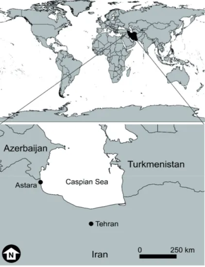
The study was conducted in the Astara port (38˚25ʹ20.84ʺ N and 48˚52ʹ07.37ʺ E) in the Western Iranian coast of the Caspian Sea (Fig. 1), from May 2015 to May 2016. This port is located on a sandy coast in the border between Iran and the Republic of Azerbaijan.

Polyvinyl Chloride (PVC) test panels (12 cm × 12 cm × 0.3 cm) were hung using 4 mm plastic ropes and suspended horizontally in 1 m depth from a pier in the Astara port. A 2 kg weight was attached underneath each panel to keep them in a stable position inside the water column. Two sets of panels were deployed. One set (hereafter refer to as STP: short-term panels) was retrieved and replaced with a new set every 2 months for a period of 12 months, in order to study recruitment patterns (5 panels per sampling event). The second set (hereafter refer to as LTP: long term-panels) was retrieved after 4, 8 and 12 months to assess the community succes- Figure 1.

408 409 410 411 412 413 414 415 416 417 418 419 420 421 422 423 424 425 426 427 428 429 430 431 432 433 434 435 436

Figure 1. Location map of the Astara port on the Western Iranian coast of the Caspian Sea, place where the current study was devel- oped.

(3)

112 Golinia et al.

sion (4 panels per sampling event). Temperature, salinity, dissolved oxygen and pH were monthly measured. Nitrate, nitrite, phosphate and chlorophyll a were measured every 2 months in the laboratory according to standard methods (Adams 1990, Eaton et al. 1995).

Samples processing

Collected panels were gently rinsed with fresh water to remove excess sediment and salt, photographed, transferred to the laboratory on ice and kept at -20 ˚C for further analy-˚C for further analy- for further analysis. Some samples were separately preserved in 70% ethyl alcohol for potential further identification. Samples were identified to the lowest possible taxonomic level based on existing literature and the expertise of local taxonomists.

To determine the coverage for each taxa, the photographs of the panels were analyzed using the software CPCe 4.1.

(Kohler and Gill 2006). Each image was sub-divided into a 3×3 grid of 9 cells, with 11 random points per cell, produc-

ing a maximum number of 99 points analyzed per picture. It is noteworthy that because of multilayer accumulation of foul- ers, coverage can be well over 100% (Canning-Clode et al.

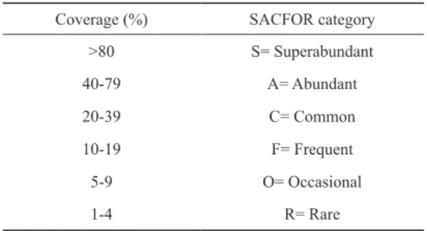
2009). Before introducing the taxon names into the software, each image was checked with its respective real panel under a stereo microscope. Since bryozoans were distinguishable from panel pictures only to the order level (Cheilostomata and Ctenostomata), their coverage was aggregated at this taxonomic level. However, bryozoans were later identified down to the species level using scanning electron microscope photographs (see Table 3 for the species names). Based on the mean coverage calculated for the overall sampling period, the SACFOR scale was used to classify fouling taxa in STP and LTP (Connor and Hiscock 1996). Classification levels included in the frame of the SACFOR scale are presented in Table 1.

In order to measure the dry weight (DW), samples were carefully scraped from the panels and placed in pre-weighed aluminum pans, dried at 60 °C in the oven for 24 hours and weighed. Samples were then burnt in a muffle furnace at 500 °C for 6 h and reweighed. By subtracting the ash weight (AW) from the DW, the ash-free dry weight (AFDW) was calculated. Inorganic to organic matter ratio was calculated by dividing the AW by the AFDW of samples. Dry weight was considered as biomass.

Data processing and statistical analyses

Temporal trends of coverage, biomass and inorganic to organic matter ratio for the whole community were analyzed using Generalized Additive Models (GAM), employing the mgcv R package (Wood and Wood 2016). Temporal trends of the coverage for the barnacle Amphibalanus improvisus, the bryozoans of the orders Cheilostomata and Ctenostomata and the green algae Schizomeris sp. (most abundant taxa) were also analyzed through GAM. The distribution and the link Table 1. SACFOR scale (Connor & Hiscock, 1996) used to clas-

sify the sampled taxa based on the mean coverage for the entire study period. Classification categories defined in the frame of the scale are presented.

Table 2. Distributions, link functions and transformations used in Generalized Additive Models for the different response variables analyzed in the present article.

Coverage (%) SACFOR category

>80 S= Superabundant

40-79 A= Abundant

20-39 C= Common

10-19 F= Frequent

5-9 O= Occasional

1-4 R= Rare

Response variable Data source Distribution Link function Transformation

Coverage of the community STP Gamma Log

LTP Gamma Log

Biomass of the community STP Gamma Log

LTP Gamma Log

Inorganic toorganic matter ratio of the community STP Gaussian Identity

LTP Gaussian Identity

Coverage of Amphibalanus improvisus STP Gaussian Identity

Coverage of Cheilostomata STP Gaussian Identity ln(y+1)

LTP Gaussian Identity ln(y+1)

Coverage of Ctenostomata STP Gaussian Identity ln(y+1)

Coverage of Schizomeris sp. STP Gaussian Identity ln(y+1)

LTP Gaussian Identity ln(y+1)

(4)

function employed in each model were selected according to the nature of the response variable (see Table 2). In those cas- es where the existing distributions and link functions were not able to properly model the response variable, the data were normalized using a logarithmic transformation. In all the models, the time in months was considered as the explanatory variable and included as a smooth term using penalized cubic regression splines with up to three degrees of freedom. The adequacy of the adjusted models was determined by checking the explained deviance and the plots of residuals.

Results

Environmental parameters

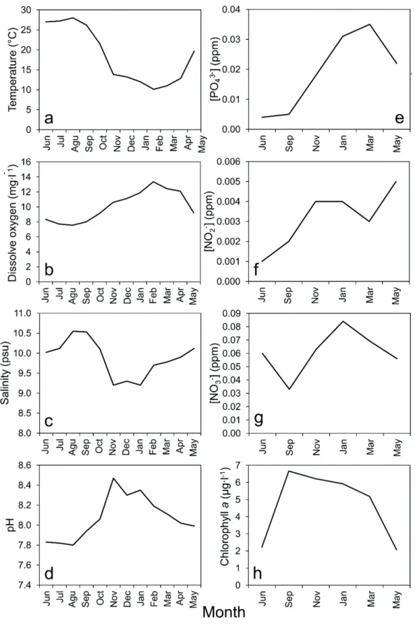
Environmental variables registered from June 2015 to May 2016 are presented in Figure 2. Water temperature ranged from 10.1 to 28 ˚C. It decreased gradually from sum-˚C. It decreased gradually from sum- It decreased gradually from summer to autumn, reached its minimum in winter and increased again during spring. Dissolved oxygen, which ranged from 7.7 to 13.35mg.l^-1, followed an opposite trend to that seen for temperature. pH was minimum (7.83) in summer and maximum (8.47) in winter. Salinity almost did not vary during the study period (9.2-10.55 psu). The lowest phosphate concen- tration (0.004 ppm) was observed in summer and the highest (0.035 ppm) in early spring. Nitrite and nitrate concentrations ranged from 0.001 (in summer) to 0.004 ppm (in spring) and from 0.033 (in summer) to 0.084 ppm (in winter), respectively. Chlorophyll a increased from early summer, reached its maximum (6.66 µg.l^-1) in late summer and decreased steadily towards spring.

Community patterns

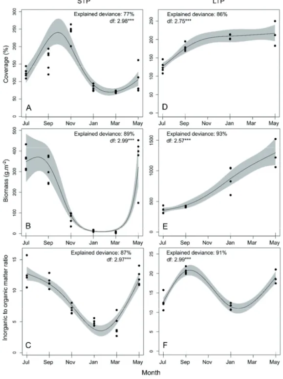
Short-term panels. Coverage, biomass and inorganic to or- ganic matter ratio of recruiting communities varied season- ally in STP. GAM showed that the mean trend of coverage increased from July to November 2015. After reaching its highest value (247.7%) by the end of summer and beginning of autumn (September-November 2015), the coverage decreased to its minimum (70.0%) during winter months (January-March 2016, Figure 3a). In contrast to coverage, biomass and inorganic to organic matter ratio already showed their maximum values (721.9 g·m^-2 and 12.7, respectively) in mid-summer (July 2015), started to decrease in September 2015 and reached the lowest values in the period January- March 2016. The taxa that recruited in the period March-May 2016 promoted a new increase in inorganic matter and a con- comitant increase of the overall biomass (Fig. 3b, c).

Long-term panels. GAM showed that the coverage in LTP increased in the period July-September 2015, after which the observed values were approximately 200% for the rest of the sampling (Fig. 3d). Biomass increased over the entire sampling period, from a mean value of 360.9 g·m^-2 in July 2015 (i.e., in 2 months old panels) to a value of 1540.6 g·m^-2 in May 2016 (12 months old panels, Fig. 3e). In contrast to the asymptotic trend observed for coverage and the continuous increase of biomass, the inorganic to organic matter ratio followed a cyclic trend (Fig. 3f). The inorganic to organic matter ratio increased from 2 to 4 months panels (during the period July-September 2015). After peaking in September 2015, it decreased in winter (January 2016, after 8 months) and increased again towards May 2016 (Fig. 3f).

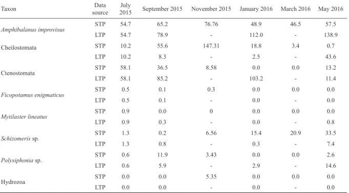
Table 3. Mean coverage of biofouling taxa observed for short-term panels (STP) and long-term panels (LTP) during the study pe- riod (from May 2015 to May 2016). The information is presented by sampling event. Note that LTP information is not available for November 2015 (6 months panels) and March 2016 (10 months panels) due to the sampling design (see details in the main text).

Taxon Data

source July

2015 September 2015 November 2015 January 2016 March 2016 May 2016

Amphibalanus improvisus STP 54.7 65.2 76.76 48.9 46.5 57.5

LTP 54.7 78.9 - 112.0 - 138.9

Cheilostomata STP 10.2 55.6 147.31 18.8 3.4 0.7

LTP 10.2 8.3 - 2.5 - 43.6

Ctenostomata STP 58.1 36.5 8.58 0.0 0.0 13.2

LTP 58.1 85.2 - 103.2 - 11.4

Ficopotamus enigmaticus STP 0.5 0.1 0.3 0.0 0.0 0.0

LTP 0.5 0.1 - 0.0 - 0.0

Mytilaster lineatus STP 0.9 0.0 0 0.0 0.0 0.0

LTP 0.9 0.3 - 0.0 - 0.8

Schizomeris sp. STP 1.3 0.2 6.56 15.4 20.9 33.5

LTP 1.3 0.8 - 0.3 - 7.4

Polysiphonia sp. STP 0.6 11.9 3.43 0.0 0.0 2.6

LTP 0.6 5.9 - 2.9 - 14.6

Hydrozoa STP 0.0 0.0 5.35 0.0 0.0 0.0

LTP 0.0 0.0 - 0.0 - 0.0

(5)

114

Figure 2.

Golinia et al.

437 438

439 440

Figure 2. Temperature (a), salinity (b), dissolved oxygen (c), pH (d), nitrite (e), nitrate (f), phosphate (g) and chlorophyll a (h) meas- ured in the Astara port from June 2015 to May 2016. The first group of variables (a-d) were measured every month, while those in the second one (e-h) were measured every 2 months. Because of some logistic issues in the second month of the sampling, there was a month of delay in the sampling of the second group of variables.

(6)

Patterns by taxa

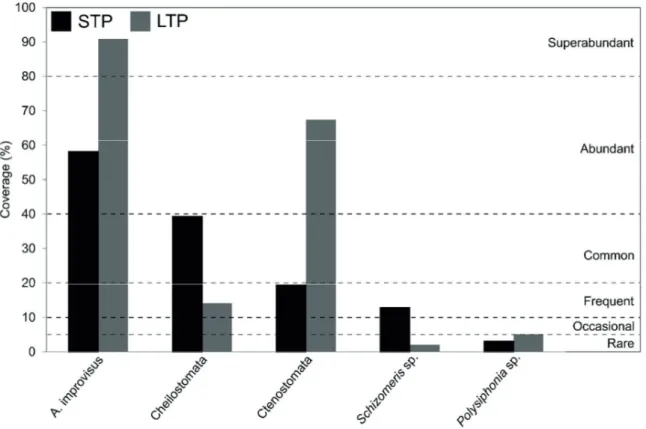
Short term panels. A total of 10 macrofaunal taxa were ob- served in STP when all sampling events were considered (Table 3). The barnacle A. improvisus occurred all-year round and was the dominant species in 4 of the 6 sampling events, only being surpassed by Ctenostomata and Cheilostomata in July 2015 and November 2015 (Table 3). Based on the

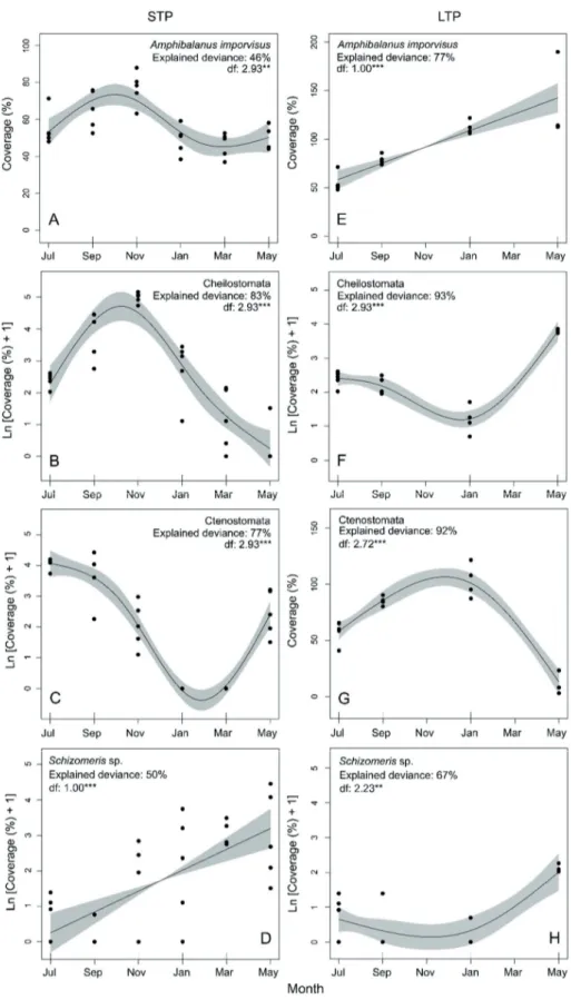
SACFOR scale, this barnacle species was classified as abundant (Fig. 4). Beyond occurring in all sampling events and showing high coverage values over the entire study, GAM showed a clear seasonal trend in A. improvisus recruitment (Fig. 5a). After steadily increasing during summer and peaking in September-November 2015, the coverage of barnacles decreased during winter and recovered in May 2016. The coverage of Cheilostomata (common taxa in STP considering

Figure 3. Temporal trends for the coverage (a, d), biomass (b, e) and inorganic to organic matter ratio (c, f) for the whole community analyzed with Generalized Additive Models. Trends obtained for short term panels (STP) and long term panels (LTP) are presented. The solid line represents the best cubic regression spline adjusted and the grey shadow shows the confidence interval at the 95%. The explained deviance and the degrees of freedom (df) of the best cubic regression spline are presented for each model. ***: p-values < 0.001.

Figure 3.

441 442 443

444

(7)

116 Golinia et al.

the SACFOR scale) followed a similar seasonal trend to that observed for A. improvisus (Fig. 5b). In contrast, the bryozoans from the order Ctenostomata exhibited the maximum coverage in the first sampling event (July 2015), decreased during autumn and winter and reached the lowest values in January-March 2016. In May 2016, the coverage of Ctenostomata recovered and showed similar values to those observed at the beginning of autumn (Fig. 5c). Ctenostomata was classified as frequent in STP based on the mean coverage registered for this taxa during the overall sampling period (Fig. 4). The Chlorophyta of the species Schizomeris sp. (frequent in STP, Fig. 4), steadily increased from July 2015 to May 2016 (Fig. 5d).

Long term panels. On average, A. improvisus linearly in- creased throughout the study period, while Cheilostomata and Ctenostomata followed non-linear trends (Fig. 5e, Table 3). The coverage of Cheilostomata was minimum in January 2016 and reached its highest values in the first and last sampling events (July 2015 and May 2016) (Fig. 5f).

The Ctenostomata coverage exhibited the opposite trend, being maximum in winter (January 2016) and minimum in July 2015 and May 2016 (Fig. 5g). In contrast to the previous taxa, the coverage of Schizomeris sp. remained almost con- stant from July 2015 to January 2016 and increased during spring (Fig. 5h). Based on the SACFOR scale, A. improvisus was classified as superabundant, the bryozoans of the orders Cheilostomata and Ctenostomata as frequent and abundant, Schizomeris sp. as rare and Polysiphonia sp. as occasional (Fig. 4).

Discussion

STP provided data on the temporal variations of early colonizers and how they determined noticeable changes in coverage, biomass and the ratio between inorganic and organic matter at the community level. The temporal variability observed in the coverage for the whole community was mostly driven by the recruitment patterns of barnacles and bryozoans (see Figs 3 and 5). Recent studies have shown that temporal changes in temperature, salinity, photoperiod and primary production influence the reproduction and recruitment of single species, and in consequence, the seasonal patterns observed in fouling communities (e.g., Pati et al. 2015, Sokołowski et al. 2017). In the present study, the total coverage in STP peaked by the end of summer and beginning of autumn, when temperature and chlorophyll a exhibited their highest values. In accordance with these results, Sokołowski et al. (2017) based on a monitoring performed in the Baltic coast of Poland, argued that the increase of temperature and light availability during spring and summer promotes the reproduction and spawning of epibenthic species, explaining a higher recruitment in summer. Similar results were observed for the barnacle A. improvisus, the dominant species in this study, which massively recruits during summer in the South Western Baltic Sea (Thomsen et al. 2010, Nasrolahi et al. 2012). The increase of chlorophyll a (a proxy of primary production and food availability) and the high water temperatures still seen at the beginning of autumn, could explain the high coverage values observed. High food availability has been Figure 4.

445 446 447

448 449 450 451 452 453 454 455 456 457 458

Figure 4. SACFOR classification of biofouling taxa based on their mean coverage for the entire sampling period (May 2015-May 2016). Only taxa with coverage higher than 1% were considered in the plot. Information for short-term (STP) and long-term (LTP) panels is presented.

(8)

Biofouling in the southern Caspian Sea 117

Figure 5. Temporal trends for the coverage of Amphibalanus improvisus (a, e), the orders of bryozoans Cheilostomata (b, f) and Ctenostomata (c, g) and the green algae Schizomeris sp. (d, h) analyzed with Generalized Additive Models. Trends obtained for short term panels (STP) and long term panels (LTP) are presented. In each model, the solid line represents the best cubic regression spline adjusted and the grey shadow the confidence interval at the 95%. The explained deviance and the degrees of freedom (df) of the best cubic regression spline is presented for each model. **: p-values<0.01, ***: p-values<0.001. Notice the logarithmic scale in b, c, d, f and h.

(9)

118 Golinia et al.

identified as a crucial factor for the dispersion, development and successful settlement in larvae as well as the accumulation of energy reserves to cover reproductive costs in adults (Todd 1998, Wołowicz et al. 2006). Coverage in STP strongly decreased in winter, when low temperatures probably promoted a decrease in metabolic and feeding rates, diminishing the energy intake and the resources availability for reproduction. Some new recruits were observed during winter, indicat- ing the presence of reproductive adults and larvae in the field.

However, many of these larvae are not physiologically com- petent in winter and therefore fail to attach and metamorphose to juvenile (Thiyagarajan et al. 2003, Nasrolahi et al. 2013).

Winter storms, which transport sediment loads, can lead to high mortalities of suspension feeders such as barnacles and bryozoans (Boyle et al. 2006, Houle 2015), contributing to the low total coverage observed in the season.

In this study, the biomass of biofoulers in STP (mostly determined by barnacles) during summer months was much higher (by a magnitude of 10) than in winter months. The rate of mechanisms such as food intake and assimilation in barnacles and many other invertebrates are strongly affected by temperature (Anderson 1994). For instance, during summer, high seawater temperatures increase metabolic rates and the feeding efficiency of barnacles (Crisp and Bourget 1985, Skinner et al. 2007). This, in turn, can cause higher growth rates and therefore higher biomasses. The increase of biomass in warmer months is in agreement with findings of previous studies on barnacles and other biofouling organisms (Greene and Grizzle 2007, Smale et al. 2011, Nasrolahi et al. 2013). During cold months, suboptimal temperatures can prolong the duration of development and enhance the energetic requirements for maintenance, which may result in smaller individuals. Likewise, low temperature postpones larval metamorphosis and dramatically depresses post-meta- morphic growth, leading to less biomass formation (Pechenik et al. 1993). The inorganic to organic matter ratio followed a similar seasonal trend as that of biomass. Organic matter (body) in STP increased at the community level from summer to winter by more than 300% over inorganic matter (shells).

Nasrolahi et al. (2013) found similar results for A. improvisus under experimental conditions, where organisms subjected to higher temperature treatments exhibited higher inorganic to organic matter ratios than those exposed to lower temperatures. Reduced food consumption as a consequence of low temperature results in less energy intake. This, in combina- tion with the fact that calcification in cold water is energeti- cally more costly (Melzner et al. 2011), determines a reduc- tion in shell production and in consequence in the inorganic to organic matter ratio in winter.

Through the analysis of coverage patterns by taxa in STP, it was possible to observe a mismatch in the seasonal trends of Cheilostomata and Ctenostomata bryozoans (see Fig. 5b, c and Table 4). Ctenostomata exhibited the highest coverage values in summer, being replaced by Cheilostomata as autumn progressed. To explain the replacement of some species (or entire groups of species) by others, reproduction and recruitment seasonality, asymmetric interspecific competition and/or the release of space by environmental dis-

turbances (among others) have been proposed as potential mechanisms [see Liow et al. (2016) and citations therein].

Several studies have shown the relevance of competitive displacement between bryozoan clades in explaining diversity patterns in paleontological records of this phylum, highlight- ing the superior competitive abilities of Cheilostomata species and the successful radiation of this order (Sepkoski et al.

2000). In light of this information, the delayed recruitment of Cheilostomata in comparison to Ctenostomata bryozoans, in addition to the capacity of Cheilostomata to displace other bryozoan clades, could explain the seasonal mismatch observed in the present study.

The results from LTP showed an asymptotic increase of coverage and a continuous increase of biomass in relation to submersion time, trends that were accompanied by a low and almost constant number of species during the overall study period (see Fig. 3 and Table 4). The dominance of barnacles and bryozoans was clearly evidenced by the similarities between coverage and biomass patterns for these taxa and the whole community. Coverage rapidly reached a ceiling in LTP, which could be explained by the continuous colonization by barnacles during the entire study period. Previous studies have shown that the amount of free space on the panels usu- ally decreases with the progression of the succession, espe- cially when early colonizers exhibit high growth rates and prevent the settlement of new ones (Benedetti-Cecchi 2000, Cifuentes et al. 2010, Lindeyer and Gittenberger 2011). The biomass of biofoulers on the LTP, ranged from 722 (after 2 months) to 2559 g·m^-2(after 12 months), being much lower than those observed in the Indian ocean, specifically for the Gulf of Oman (4-months age panel, wet weight: 6000 g·m^-2, Dobretsov et al. 2015) and the Bay of Bengal (6-month age panel, wet weight: 6392 g·m^-2, Pati and Rao 2015).

Succession patterns can differ depending on the season when the sampling structures are deployed (Underwood and Anderson 1994, Satheesh and Wesley 2011). Despite the fact that all the panels were deployed in May 2015, the dominance of barnacles over almost the entire year and the absence of strong competitors (like mussels) lead to the prediction that the patterns observed for STP and LTP in this study would most likely not vary if the panels had been initially deployed in a different season. Thus, the information generated in this study represents a reliable baseline for future studies and management strategies dealing with biofouling issues in the Caspian Sea. However, studying the biofouling assemblages in LTP at various starting seasons and for several years would generate more conclusive results.

Conclusions

Our data showed tremendous temporal variations in the recruitment of biofouling communities of the Caspian Sea.

In this low diversity region, barnacles and bryozoans were the main determinants of recruitment and successional patterns. These patterns followed temperature and chlorophyll a trends, factors that strongly influence survival, growth and reproduction of fouling species, and in consequence the structure of assembled communities.

(10)

As shipping and the number of marine anthropogenic structures continue to increase and predictive scenarios in- dicate that fouling pressure will likely be enhanced by global warming (Poloczanska and Butler 2010), the study of biofouling and its economic consequences have never been more in force. In this context, the present study only represents the starting point for future long-term monitoring efforts of biofouling communities in the Caspian Sea, a place where this topic has been thoroughly overlooked.

Acknowledgements: We would like to thank the head and guard officers of the Astara Port Special Economic Zone for issuing the sampling permission. FRB acknowledges the Deutscher Akademischer Austauschdienst (DAAD) for finan- cial support to pursue his PhD

References

Adams, V.D. 1990. Chemical oxygen demand (COD) ampule meth- od. In: Water and Wastewater Examination Manual. CRC Press, Florida. pp. 173–177.

Anderson, D.T. 1994. Barnacles: Structure, Function, Development and Evolution. Chapman and Hall, London.

Balaji, M. and K.S. Rao. 2004. Biofouling communities as tools in environmental impact assessment - A study at Visakhapatnam harbour, east coast of India. Asian J. Microbiol. Biotechnol.

Environ. Sci. 6:223–229.

Benedetti-Cecchi, L. 2000. Predicting direct and indirect interactions during succession in a mid‐littoral rocky shore assemblage. Ecol.

Monogr. 70:45–72.

Boyle, M.D., S.C. Janiak and S. Craig. 2006. Succession in a Humboldt Bay Marine Fouling community: the role of exotic species, larval settlement and winter storms. In: Proceedings of the 2004 Humboldt Bay Symposium. pp. 215-234.

Canning-Clode, J., N. Bellou, M.J. Kaufmann and M. Wahl. 2009.

Local–regional richness relationship in fouling assemblages–effects of succession. Basic Appl. Ecol. l10:745–753.

Canning-Clode J., H. Sugden. 2014. Assessing fouling assemblages. In: S. Dobretsov, D.N. Williams and J.C. Thomason, (eds.), Biofouling Methods. Wiley, Chichester. pp. 252-271.

Cao S., J. Wang, H. Chen and D. Chen. 2011. Progress of marine biofouling and antifouling technologies. Chin. Sci. Bull. 56:598–

612.

Cifuentes M, I. Krueger, C.P. Dumont, M. Lenz and M. Thiel. 2010.

Does primary colonization or community structure determine the succession of fouling communities? J. Exp. Mar. Biol. Ecol.

395:10–20.

Coetser S.E. and T.E. Cloete. 2005. Biofouling and biocorrosion in industrial water systems. Crit. Rev. Microbiol. 31:213–232.

Connor, D. and K. Hiscock. 1996. Data collection methods. In:

K. Hiscock (ed.), Marine Nature Conservation Review:

Rationale and Methods. Joint Nature Conservation Committee, Peterborough. pp. 51–65.

Crisp, D.J. and E. Bourget. 1985. Growth in barnacles. Adv. Mar.

Biol. 22:199–244.

Dobretsov, S. 2015. Biofouling on artificial substrata in Muscat waters. JAMS. 19:24 – 29.

Eaton, A.D., L.S. Clesceri and A.E. Greenberg. 1995. Standard Methods for the Examination of Water and Wastewater. American Public Health Association, Washington, DC.

Fitridge, I., T. Dempster, J. Guenther and R. de Nys. 2012. The impact and control of biofouling in marine aquaculture: a review.

Biofouling 28:649–669.

Greene, C.H. and A. Schoener. 1982. Succession on marine hard substrata: a fixed lottery. Oecologia 55:289–297.

Greene, J.K. and R.E. Grizzle. 2007. Successional development of fouling communities on open ocean aquaculture fish cages in the western Gulf of Maine, USA. Aquaculture 262:289–301.

Houle, K.C. 2015. The effects of suspended and accreted sediment on the marine invertebrate fouling community of Humboldt Bay.

Humboldt State University, Arcata, California.

Jenkins, S.R. and G.M. Martins. 2010. Succession on hard substrata. In: J.C. Thomason and S. Duerr (eds.), Biofouling. Wiley- Blackwell, Oxford, UK, pp. 60–72.

Kohler, K.E. and S.M. Gill. 2006. Coral Point Count with Excel ex-Coral Point Count with Excel ex- tensions (CPCe): A Visual Basic program for the determination of coral and substrate coverage using random point count meth- odology. Comput. Geosci. 32:1259–1269.

Krohling, W., D.S. Brotto and I.R. Zalmon. 2006. Fouling community recruitment on an artificial reef in the north coast of Rio de Janeiro State. J. Coast. Res. 1:1118–1121.

Lin, H.J. and K.T. Shao. 2002. The development of subtidal fouling assemblages on artificial structures in Keelung Harbor, Northern Taiwan. Zool. Stud. 41:170–181.

Lindeyer, F. and A. Gittenberger. 2011. Ascidians in the succession of marine fouling communities. Aquatic Invasions 6:421–434.

Liow, L.H., E. Di Martino, K.L. Voje, S. Rust and P.D. Taylor. 2016.

Interspecific interactions through 2 million years: are competitive outcomes predictable? Proc. Royal Soc. B. 283:20160981.

Maggiore, F. and E. Keppel. 2007. Biodiversity and distribution of polychaetes and molluscs along the Dese estuary (Lagoon of Venice, Italy). Hydrobiologia 588:189–203.

Masi, B.P., R. Coutinho and I. Zalmon. 2015. Successional trajectory of the fouling community on a tropical upwelling ecosystem in southeast Rio de Janeiro, Brazil. Braz. J. Oceanogr. 63:161–168.

Melo, L.F. and T.R. Bott. 1997. Biofouling in water systems. Exp.

Therm. Fluid Sci. 14:375–381.

Melzner, F., P. Stange, K. Trübenbach, J. Thomsen, I. Casties, U.

Panknin, S.N. Gorb and M.A. Gutowska. 2011. Food supply and seawater pCO2 impact calcification and internal shell dissolution in the blue mussel Mytilus edulis. PLoS One 6:e24223.

Minchinton, T.E. and R.E. Scheibling. 1991. The influence of larval supply and settlement on the population structure of barnacles.

Ecology 72(5):1867–1879.

Nandakumar, K. 1996. Importance of timing of panel exposure on the competitive outcome and succession of sessile organisms. Mar.

Ecol. Prog. Ser. 131:191–203.

Nandakumar, K., M. Tanaka and T. Kikuchi. 1993. Interspecific competition among fouling organisms in Tomioka Bay, Japan. Mar.

Ecol. Prog. Ser. 31:43-50.

Nasrolahi, A., C. Pansch, M. Lenz and M. Wahl. 2012. Being young in a changing world: how temperature and salinity changes interactively modify the performance of larval stages of the barnacle Amphibalanus improvisus. Mar. Biol. 159:331–340.

Nasrolahi, A., C. Pansch, M. Lenz and M. Wahl. 2013. Temperature and salinity interactively impact early juvenile development: a bottleneck in barnacle ontogeny. Mar. Biol. 160:1109–1117.

Ong, J.L.J. and K.S. Tan. 2012. Observations on the subtidal fouling community on jetty pilings in the Southern Islands of Singapore.

In: K.S. Tan (ed.), Contrib. Mar. Sci. National University of Singapore, pp. 121–126.

(11)

120 Golinia et al.

Pati, S.K. and M.V. Rao. 2015. Fouling load in a tropical Indian harbor: spatial and temporal pattern. J. Mar. Biol. Assoc. India 57:6.

Pati, S.K., M.V. Rao and M. Balaji. 2015.Spatial and temporal changes in biofouling community structure at Visakhapatnam harbour, east coast of India. Trop. Ecol. 56:139–154.

Pechenik, J.A., D. Rittschof and A.R. Schmidt. 1993. Influence of delayed metamorphosis on survival and growth of juvenile barnacles Balanus amphitrite. Mar. Biol. 115:287–294.

Pinnegar, J. K., N. V. C. Polunin, P. Francour, F. Badalamenti, R.

Chemello, M.L. Harmelin-Vivien, B. Hereu, M. Milazzo, M.

Zabala, G. d’Anna and C. Pipitone .2000. Trophic cascades in benthic marine ecosystems: lessons for fisheries and protected- area management. Environ. Conserv. 27:179–200.

Poloczanska, E.S. and A.J. Butler. 2010. Biofouling and climate change. In: S. Dürr and J.C. Thomason (eds.), Biofouling. Wiley- Blackwell, UK. pp. 333-347.

Rajagopal, S., K.V.K. Nair, G. Van der Velde and H.A. Jenner. 1997.

Seasonal settlement and succession of fouling communities in Kalpakkam, east coast of India. Neth. J. Aquat. Ecol: 30:309–

325.

Relini, G., M. Relini, G. Torchia and G. De Angelis. 2002. Trophic relationships between fishes and an artificial reef. ICES J. Mar.

Sci. 59:S36–S42.

Ruiz, G.M., T. Huber, K. Larson, L. McCann, B. Steves, P. Fofonoff and A.H. Hines. 2006. Biological Invasions in Alaska’s Coastal Marine Ecosystems: Establishing a Baseline. Final Report.

Prince William Sound Regional Citizens’ Advisory Council and U.S. Fish and Wildlife Service, Anchorage, Alaska.

Satheesh, S. and S. Godwin Wesley. 2008. Seasonal variability in the recruitment of macrofouling community in Kudankulam waters, east coast of India. Estuar. Coast. Shelf Sci. 79:518–524.

Satheesh, S. and S.G. Wesley. 2011. Influence of submersion season on the development of test panel biofouling communities in a tropical coast. Estuar. Coast. Shelf Sci. 94:155–163.

Schultz, M.P., J.A. Bendick, E.R. Holm and W.M. Hertel. 2011.

Economic impact of biofouling on a naval surface ship.

Biofouling 27:87–98.

Sepkoski Jr, J.J., F.K. McKinney and S. Lidgard. 2000. Competitive displacement among post-Paleozoic cyclostome and cheilo- stome bryozoans. Paleobiology 26:7–18.

Skinner, L.F., F.N. Siviero and R. Coutinho. 2007. Comparative growth of the intertidal barnacle Tetraclita stalactifera (Thoracica: Tetraclitidae) in sites influenced by upwelling and tropical conditions at the Cabo Frio region, Brazil. Rev. Biol.

Trop. 55:71–78.

Smale, D.A., T. Wernberg, L.S. Peck and D.K.A. Barnes. 2011.

Turning on the heat: ecological response to simulated warming in the sea. PLoS One 6:e16050.

Sokołowski, A., M. Ziółkowska, P. Balazy, P. Kuklinski and I.

Plichta. 2017. Seasonal and multi-annual patterns of colonisation and growth of sessile benthic fauna on artificial substrates in the brackish low-diversity system of the Baltic Sea. Hydrobiologia 790:183-200.

Sutherland, J.P. and R.H. Karlson. 1977. Development and stabil- ity of the fouling community at Beaufort, North Carolina. Ecol.

Monogr. 47:425–446.

Thiyagarajan, V., T. Harder, J.W. Qiu and P.Y. Qian. 2003. Energy content at metamorphosis and growth rate of the early juvenile barnacle Balanus amphitrite. Mar. Biol. 143:543–554.

Thomsen J., M.A. Gutowska, J. Saphörster, A. Heinemann, K.

Trubenbach, J. Fietzke, C. Hiebenthal, A. Eisenhauer, A.

Kortzinger, M. Wahl and F. Melzner. 2010. Calcifying inver-2010. Calcifying invertebrates succeed in a naturally CO2-rich coastal habitat but are threatened by high levels of future acidification. Biogeosciences 7:3879–3891.

Todd, C.D. 1998. Larval supply and recruitment of benthic invertebrates: do larvae always disperse as much as we believe?

Hydrobiologia 132:1–21.

Underwood, A.J. and M.J. Anderson. 1994. Seasonal and temporal aspects of recruitment and succession in an intertidal estuarine fouling assemblage. J. Mar. Biol. Assoc. U.K. 74:563–584.

Wołowicz, M., A. Sokołowski, A.S. Bawazir and R. Lasota. 2006.

Effect of eutrophication on the distribution and ecophysiology of the mussel Mytilus trossulus (Bivalvia) in southern Baltic Sea (the Gulf of Gdańsk). Limnol. Oceanogr. 51:580–590.

Wood, S. and M.S. Wood. 2016. Package “mgcv.” R package ver- sion 1–7

Yebra, D.M., S. Kiil and K. Dam-Johansen. 2004. Antifouling technology—past, present and future steps towards efficient and environmentally friendly antifouling coatings. Prog. Org. Coat.

50:75–104.

Zevina, G.B., I.A. Kuznetsova and I.V. Starostin. 1965. The status of marine fouling in the Caspian Sea. In: I.V. Starostin (ed.), Marine Fouling and Borers. USSR Academy of Sciences Trans .of the Institute of Oceanology 49 (Israel translation 1968) Zhang, H., W. Cao, Z. Wu, X. Song, J. Wang and T. Yan. 2015.

Biofouling on deep-sea submersible buoy systems off Xisha and Dongsha Islands in the northern South China Sea. Int.

Biodeterior. Biodegradation 104:92–96.

Received February 18, 2018 Revised April 18, 2018 Accepted June 1, 2018 Open Access statement. This is an open-access arti- cle distributed under the terms of the Creative Commons Attribution-NonCommercial 4.0 International License (htt- ps://creativecommons.org/licenses/by-nc/4.0/), which per- mits unrestricted use, distribution, and reproduction in any medium for non-commercial purposes, provided the original author and source are credited, a link to the CC License is provided, and changes – if any – are indicated.