On the separation between inorganic and organic fractions of suspended matter in a marine coastal
environment
M. Schartaua,∗, R. Riethmüllerb,∗∗, G. Flöserb, J. E. E. van Beusekomb, H. Krasemannb, R. Hofmeisterb, K. Wirtzb
aGEOMAR Helmholtz Centre for Ocean Research Kiel
bHelmholtz-Zentrum Geesthacht, Centre for Materials and Coastal Research
Abstract
A central aspect of coastal biogeochemistry is to determine how nutrients, lithogenic- and organic matter are distributed and transformed within coastal and estuarine envi- ronments. Analyses of the spatio-temporal changes of total suspended matter (TSM) concentration indicate strong and variable linkages between intertidal fringes and pelagic regions. In particular, knowledge about the organic fraction of TSM provides insight to how biogenic and lithogenic particulate matter are distributed in suspension. In our study we take advantage of a set of over 3000 in situ Loss on Ignition (LoI) data from the Southern North Sea that represent fractions of particulate organic matter (POM) relative to TSM (LoI≡POM:TSM). We introduce a parameterization (POM-TSM model) that distinguishes between two POM fractions incorporated in TSM. One fraction is described in association with mineral particles. The other represents a seasonally varying fresh pool of POM. The performance of the POM-TSM model is tested against data derived from MERIS/ENVISAT-TSM products of the German Bight. Our analysis of remote sensing data exhibits specific qualitative features of TSM that can be attributed to distinct coastal zones. Most interestingly, a transition zone between the Wadden Sea and seasonally strati- fied regions of the Southern North Sea is identified where mineral associated POM appears in concentrations comparable to those of freshly produced POM. We will discuss how this transition is indicative for a zone of effective particle interaction and sedimentation.The dimension of this transition zone varies between seasons and with location. Our proposed POM-TSM model is generic and can be calibrated against in situ data of other coastal regions.
Keywords: Total suspended matter (TSM), Loss on Ignition, Particulate organic matter (POM), Particulate inorganic matter (PIM), Ocean color, Coastal
biogeochemistry
∗First corresponding author
∗∗Second corresponding author
Email addresses: mschartau@geomar.de(M. Schartau),rolf.riethmueller@hzg.de (R. Riethmüller)
Highlights
• Two types of organic matter inferred from total suspended matter concentration
• Organic matter is mainly mineral associated at high suspended matter concentra- tions
• Freshly produced organic matter dominates at low suspended matter concentrations
• Spatial patterns in organic matter types reveal coastal transition zones
• Specific zones for particle interaction and sedimentation can be identified
1. Introduction
1
Oceanographic observations of coastal- and shallow shelf regions often reveal
2
variability that is well pronounced on local and regional scales. In addition
3
to explaining the variability of the physical dynamics, it is also of interest
4
to understand changes in the biogeochemical characteristics of the coastal
5
waters (e.g. Kallis and Butler, 2001; Hering et al., 2010). Therefore, coastal
6
science is in many cases concerned with the quantitative and qualitative
7
determination of suspended matter (e.g. Eisma, 1981; Eisma and Irion,
8
1988). In literature the term “suspended matter” (e.g. Postma, 1981) is also
9
referred to as suspended particulate matter (SPM, e.g. Sundby, 1974), or
10
total suspended solids (TSS, e.g. Daphne et al., 2011). Many recent remote
11
sensing studies involve analyses of concentrations of total suspended matter
12
(TSM, e.g. Ouillon et al., 2008; Petus et al., 2010). Since the notion “TSM”
13
is clear and unambiguous we adopt this terminology for our study.
14
Changes in TSM concentrations are associated with the dispersion of
15
river loads, tidal transport, and resuspension of biogenic and lithogenic sed-
16
iments (Postma, 1954). On seasonal scale, variability in TSM is enhanced
17
photoautotrophy (build-up of organic matter) versus heterotrophy (trans-
19
formation and decay of organic matter) in coastal zones is sensitive to light
20
availability (Cloern et al., 2014), which in turn depends on the TSM con-
21
centration. In this respect, analyses of the composition of TSM can provide
22
important constraints for the estimation of mass exchange rates, e.g. of
23
carbon, nitrogen, or phosphorus between shallow coastal zones and adja-
24
cent shelf regions (Meybeck, 1982; Sundby et al., 1992; Smith et al., 2001;
25
Van Beusekom and De Jonge, 2002; Cloern et al., 2014). Regional gradi-
26
ents and patterns of quantitative and qualitative variations of TSM may
27
disclose information about the concurrence of physical-, chemical- and bi-
28
ological processes that leave an imprint on mass flux, including sediment
29
transport, long-term morphodynamics, and biogeochemistry.
30
Early mass flux and budget calculations of TSM have been done for the
31
Gulf of St. Lawrence (Sundby, 1974), the North Sea (Postma, 1981; Eisma
32
and Kalf, 1987; Eisma and Irion, 1988), or for the German Bight (Puls et al.,
33
1997). In these studies the TSM’s qualitative characteristics, e.g. grain-size,
34
helped consolidating mass inventories. Likewise, origin and fate of matter
35
in estuarine turbidity maximum zones can be better identified by measuring
36
the quality of TSM, as done for example in the Humber-Ouse estuary (Uncles
37
et al., 2006) or Elbe estuary (Van Beusekom and Brockmann, 1998). The
38
portion of particulate organic matter (POM) of TSM is of particular interest,
39
e.g. when investigating organic matter incorporation into sediments and its
40
preservation therein (e.g. Keil et al., 1994; Mayer, 1994; Arnarson and Keil,
41
2001), or when analysing sorption of dissolved organic carbon (Middelburg
42
and Herman, 2007) or of trace elements (Nyeffeler et al., 1984; Comber et al.,
43
1996; Garnier et al., 2006) on particles.
44
The percentage of organic matter of TSM can be determined by a gravi-
45
metric method, based on consecutive measurements of the particulate mat-
46
ter retained on individual filters. This method involves the combustion of
47
organic matter and it is referred to as Loss-on-Ignition (LoI). For marine
48
sediments, Wang et al. (2011) found that this method yields reliable results
49
as long as certain temperature and duration ranges are obeyed and identical
50
protocols in the lab procedures are followed. However, the chemical analy-
51
ses of in situ TSM field samples is laborious, which demands a trade-off in
52
sampling effort and thus in spatio-temporal resolution.
53
Horizontal spatial and temporal patterns of TSM can be well resolved
54
from remote sensing, although cloud coverage impairs the availability of
55
usable measurements. Also, the tidal dynamics remain largely unresolved
56
(no more than two satellite overflights per day per region), and processes
57
along the vertical such as mixing, settling, and resuspension may also be
58
undetected. In spite of these limitations, remote sensing data are indis-
59
pensable. Available remote sensing TSM data products typically represent
60
a bulk quantitative measure, but it is desirable to obtain qualitative infor-
61
mation from these products as well. During the past years, analyses of the
62
waters’ inherent optical properties (IOPs) have advanced the description of
63
qualitative TSM characteristics in coastal areas (e.g. Babin and Stramski,
64
2004; Stavn and Richter, 2008; Martinez-Vicente et al., 2010; Zhang et al.,
65
2014; Woźniak, 2014). Stavn and Richter (2008) proposed a discrimina-
66
tion between mass-specific scattering cross-sections that allows distinguish-
67
ing between particulate inorganic matter (PIM) and POM. An alternative
68
approach to analysing IOPs is to establish a mathematical relationship for
69
the estimation of PIM and POM concentrations, based onin situTSM and
70
content as a function of TSM concentration (POM-TSM model). We take
73
advantage of a large number of in situ LoI measurements collected in the
74
southern North Sea, mainly within the German Bight. With these obser-
75
vations we derived a model that describes predominant changes seen in the
76
LoI data. After calibration, the model can be applied to estimate POM
77
from bulk TSM concentration measurements of those devices that do not
78
detect POM explicitly, e.g. from in situ turbidity sensors or from remote
79
sensing products. Such POM estimates can support analyses of fluorescence
80
measurements and the POM-TSM model may also be used to complement
81
analyses of IOPs. We treat the measured LoI as a mixed signal of two inher-
82
ently different POM fractions, similar to distinctions proposed by Ittekkot
83
(1988) for riverine particulate organic carbon (POC): one is associated with
84
sediment minerals (e.g. Keil et al., 1994) and another is attributed to the
85
seasonal build-up and decay of “fresh” organic biomass.
86
The proposed POM-TSM model is represented by a simple equation
87
with two parameters. Maximum likelihood (ML) estimates of parameter
88
values are determined by using data of specified periods, for Spring/bloom,
89
Summer/post-bloom, and for Fall/winter respectively. We seek to make in-
90
ference about the differences between optimal parameter estimates obtained
91
for these seasons. The usability of the calibrated POM-TSM model is ex-
92
emplified by applying it to remote sensing data of TSM concentration in the
93
German Bight for the years 2010 and 2011 (2008 and 2009 are available as
94
supplemental material). We will discuss the mixing model of Morris et al.
95
(1987); an approach that has often been used to describe the POC fraction
96
of TSM. Potential improvements of our static POM-TSM model will be elu-
97
cidated, while discussing how temporal and spatial variations of the model’s
98
parameter values can be accounted for.
99
2. Methods
100
2.1. TSM concentration and Loss on Ignition (LoI) from water samples
101
The water sample data (N=3600) considered here are publicly available in
102
the World Data Center PANGAEA (https://pangaea.de/ ) (Riethmüller and
103
Flöser, 2017), including a detailed documentation of the sampling and filter-
104
ing methods. The available full data set also comprises measurements of the
105
MaBenE project (Herman, 2006) from locations in the Oosterscheldt, Lim-
106
fjorden, and Ria de Vigo (N=225). These MaBenE data were excluded and
107
we used only those samples that were taken during numerous field surveys
108
between the years 2000 and 2015 in several parts of the German Wadden
109
Sea, the Exclusive Economic Zone of Germany in the German Bight, south-
110
ern North Sea (Fig.1). This gives us a total of N=3375 water samples for
111
calibrations and analyses. The MaBenE measurements are considered for
112
our discussion of the POM-TSM model’s portability. The sampling areas
113
and the number of samples per area are listed in Table 1. Over the years,
114
the laboratory methods and the type of filter (Whatman GF/C glass fibre
115
filter, 47 mm diameter) were kept identical, but the sampling methods were
116
adapted to technical demands, to the specific conditions of the sampling
117
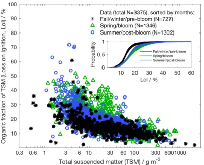
areas.
118
About 800 samples (24 % of all data) before June 2003 were taken with
119
a suction bottle sampler. From then onwards, the vast majority (62 %) of
120
samples was taken by an on-board pump. In both cases, a sample bottle was
121
filled with about 1 dm3 in 30 seconds. 260 samples in the Wadden Sea were
122
taken with an automated pump system installed on a permanent measuring
123
of 1 minute for 2 dm3 of water. To assure the homogeneity of the overall
126
data set, parallel sampling with the different methods was carried out. No
127
systematic differences in the relation of LoI to TSM were detected. Overall,
128
the sampling heights ranged from 1 m below surface to 1 m above seabed.
129
Further details about sampling and lab methods are given in Riethmüller
130
and Flöser (2017).
131
For each sample, TSM concentration and LoI were determined using
132
the same filter. Prior to sampling, the filters were flushed with deionized
133
water, heated to 525o Celsius for one hour in a muffle furnace and weighed
134
(filter dry weight). Vacuum filtration was carried out within 2 hours after
135
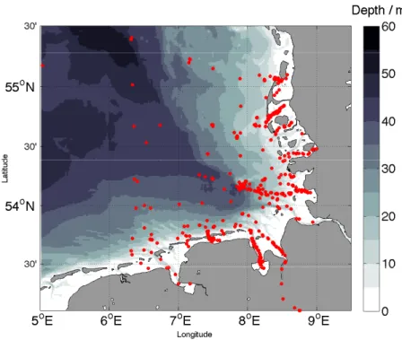
Figure 1: Bathymetry of the south-eastern part of the North Sea and locations of in situTSM and LoI measurements in the German Bight (marked red). Depths are given in meters with respect to Normal Chart Datum.
Table 1: Regions and number of available samples of Loss on Ignition (LoI) and total suspended matter (TSM) concentration measurements, as used for our analyses. See Figure 1 for the exact locations of sampling.
Region Number of samples
East Frisian Wadden Sea 1195 North Frisian Wadden Sea 1536 Estuaries Weser, Ems, Elbe 96
German Bight 548
All 3375
sampling and the filters were frozen immediately after filtering down to -18o
136
Celsius until laboratory analysis. In cases of expected long filtration times
137
(>4 h per filter) at higher TSM concentrations (typically above 50 g m−3)
138
and/or clogging of filters by fine suspended particles, the sampled water was
139
filtered through two to four parallel filters, keeping the filtering times within
140
reasonable limits. For the same reason, at very high TSM concentrations
141
(typically above 100 g m−3) only representative subsamples of the collected
142
water were filtered. In this case, the full sample was divided into halves or
143
two times into quarters by pouring the gently rotated water bottle into a
144
filter hopper with four outlets at the bottom, thus filling two bottles from
145
each two opposite outlets. After filtering the sea water sample, the loaded
146
filters were flushed with 120 cm3of deionized water to remove the remaining
147
salt from the filter. For determination of the TSM concentration, the loaded
148
filters were dried in a microwave oven for 60 minutes and weighed afterwards.
149
nearly all organic carbon was burned while the loss of carbon from volatile
152
inorganic compounds is minimized. However, the combustion duration was
153
shorter than recommended by Wang et al. (2011), which may have created
154
some small negative bias in the LoI. At the same time, this effect was found
155
to be reproducible as long as identical protocols are followed. Eventually,
156
the combusted filters are weighed again. Röttgers et al. (2014) have recently
157
shown that significant and contradictory bias errors may still remain despite
158
washing with deionized water, due to filter material loss during washing and
159
combustion procedures. To determine the net loaded filter weight offsets
160
on an individual sample basis they proposed filtering several different sub-
161
volumes of the same sample. As this method was not applied to all samples
162
presented here, a statistical overall correction was assigned to filter weights.
163
Since Röttgers et al. (2014) used Whatman GF/F glass-fibre filters in
164
their investigations, we repeated the determination of filter offsets for GF/C
165
filters, with additional 30 water samples where four sub-volumes were fil-
166
tered, following the procedures described therein. The average offset for
167
loaded filters was 0.22 mg (standard deviation 0.38 mg) and for combusted
168
filters 0.47 mg (standard deviation 0.22 mg). TSM concentration and LoI
169
were defined and calculated according to the following formulae:
170
TSM =
Nf
X
i=1
(Floaded−Fempty)i−Nf·FcorrL
Nf
X
i=1
(Vfiltered)i
(1)
and
LoI ≡
Nf
X
i=1
(Floaded−Fcombusted)i−Nf ·FcorrC
Nf
X
i=1
(Floaded−Fempty)i
( ·100[%] ) (2)
whereNf is the number of filters per sample, Fempty the dried empty filter
171
weight,Floadedthe dried loaded filter weight,FcorrLthe average dried loaded
172
filter offset, Vfiltered the filtered sample volume, Fcombusted the combusted
173
filter weight, andFcorrC the average combusted filter offset. This correction
174
reduces TSM concentrations typically by 0.3 g m−3 at 3 g m−3 and 0.4 g
175
m−3 at 30 g m−3.
176
Finally, the bias introduced by loss of structural water was corrected
177
according to Barillé-Boyer et al. (2003). Their formula requires the clay
178
content and clay composition of the suspended particles. For the German
179
Bight, Wadden Sea, Elbe and Weser estuaries these have been taken from
180
data collected by Irion and Zöllmer (1999). The correction lowers the mea-
181
sured LoI. It increases with the inorganic fraction of the suspended particles,
182
i.e. generally with the TSM concentration and amounts to 3 % at TSM con-
183
centration of 3 g m−3 and 13 % at 30 g m−3. For the other sampling areas,
184
comparable data were not available. As this correction is minor and reveals
185
Each sample had to pass four tests before it was accepted for the analysis:
188
i) the sampler did not touch the ground before sampling, ii) no loss of wa-
189
ter during filtering, iii) the sampling location had to be at a clear distance
190
from dump sites, iv) the filter weights had to be consistent, thereby reject-
191
ing cases of incorrectly transcribed filter weights. For each sample, the final
192
methodological error in TSM concentration and LoI was individually com-
193
puted applying Gaussian error propagation to Eq.(2). These calculations
194
include the weighing errors and uncertainties in the respective offsets of the
195
dried and burned loaded filters. Samples with TSM concentrations above
196
50 g m−3 yield relative errors for TSM in the order of 1 %. Concentrations
197
below 50 g m−3 result in relative errors that gradually approach 15 % with
198
decreasing TSM concentration. For LoI, the errors depend on the TSM con-
199
centration as well as on the LoI: for TSM concentrations above 50 g m−3,
200
the LoI relative error is below 1 %, at 3 g m−3, the error ranges between 2
201
and 6 % with decreasing TSM concentration.
202
For our analysis we sorted all our German Bight/Wadden Sea in situ
203
measurements (Nall = 3375) according to distinct periods of the year. This
204
way we obtained three different seasonal data subsets: a) Fall/winter/pre-
205
bloom (October through March, Nw= 727), b) Spring/bloom (April through
206
June, Nb = 1346), and c) Summer/post-bloom (July through September,
207
Ns = 1302). Fig.2 shows all data subsets of LoI measurements versus TSM
208
concentration. Probability density estimates of the seasonal data subsets
209
were calculated with a bootstrap procedure (taking 100 subsamples from
210
every data subset). The corresponding ensembles of empirical cumulative
211
probability density estimates are used to evaluate differences between the
212
seasonal data subsets, shown as subplot in Fig.2.
213
Figure 2: Organic fraction of total suspended matter (TSM), based on Loss on Igni- tion measurements (LoIobs), versus the corresponding TSM concentration. All data are sorted according to seasonal periods: a) Fall/winter/pre-bloom (October through March, black asterisks), b) Spring/bloom (April through June, green triangles), and c) Summer/post-bloom (July through September, blue circles). The subplot depicts empirical cumulative probability density functions (bootstrapped by taking 100 sub- samples), showing the statistical differences between the seasonally sorted data sets.
2.2. Remote sensing data of TSM concentration
214
The remote sensing data of TSM concentrations were derived from measure-
215
ments by MERIS (Medium Resolution Imaging Spectrometer) on ENVISAT,
216
the Environmental Satellite of the European Space Agency. ENVISAT was
217
in operation from the year 2002 until May in 2012. The MERIS is a passive
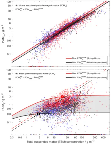
218
push broom spectrometer of the full spectrum from violet to near infrared,
219
the algorithms MEGS 8.1 (equivalent to the IPF 6.04, Instrument Process-
222
ing Facility), which are equivalent to MERIS 3rd reprocessing. For coastal
223
waters a specific processing branch is applied, according to Doerffer and
224
Schiller (2007) and Doerffer (2011), namely the C2R (Case-2 Regional pro-
225
cessor, version 1.6.2, 2010) with a coupled atmospheric correction and in
226
water constituent retrieval procedure for Case-2 water, see Appendix A1 for
227
more details.
228
We collected all available MERIS scenes over the North Sea. Individ-
229
ual pixels to which TSM concentrations could be assigned indicate a valid
230
processing. However, for our study here we excluded those pixels from the
231
analyses where the water column is shallower than 5 meters in depth to
232
avoid effects from bottom reflectance that are not taken into account by
233
the algorithm. We sorted processed scenes by months for the years 2008
234
through 2011, having typically around twenty scenes available for individ-
235
ual months. For each month we calculated mean TSM concentrations for
236
those pixels that have at least four values assigned (no clouds) within the
237
respective month. Although available, all scenes from November through
238
February have been excluded from our analysis. The low inclination of the
239
solar irradiance at these latitudes during winter in combination with very
240
low TSM concentrations within the deeper pelagic regions enhance uncer-
241
tainties in resolving coherent spatial patterns, from the shallow coastal zones
242
to the deeper areas of the German Bight. In the end we analysed mean TSM
243
scenes for the months March through October, from 2008 through 2011.
244
3. Theory
245
A LoI value expresses the relative fraction of POM for a corresponding
246
measured TSM concentration (LoI≡POM:TSM). Fig.2 reveals a sigmoidal
247
increase in LoI measurements with decreasing TSM concentration. Most of
248
our data of the German Bight exhibit TSM concentrations above 1 g m−3,
249
with only four winter measurements where TSM varies between 0.5 and 1
250
g m−3. Our LoI data typically approach maximum values between 0.5 and
251
0.7 (50 and 70 %) at the low range of TSM concentrations (<5 g m−3). LoI
252
shows little variations at high TSM concentrations (>200 g m−3), indicating
253
a prevailing organic fraction between 3 and 13 %. The transition from low
254
to high organic fractions of TSM or of the respective organic carbon content
255
is a robust qualitative feature that has been observed in many studies in
256
the past within different coastal, estuary and riverine regions (e.g. Manheim
257
et al., 1972; Eisma and Kalf, 1987; Ittekkot and Laane, 1991). Motivated
258
by these characteristics, we devised a relationship between LoI and TSM
259
concentration (POM-TSM model), which will be explained stepwise.
260
3.1. Differentiation between particulate inorganic- and organic suspended
261
matter
262
TSM can be partitioned into particulate inorganic matter (PIM) and parti-
263
cluate organic matter (POM):
264
TSM =PIM+POM (3)
Each of the two major fractions (PIM and POM) can be split up further, as
265
described in the following.
266
3.1.1. Lithogenic and biogenic particulate inorganic matter
267
PIM in coastal sea regions consists of lithogenic particles (PIMl) and bio-
268
genic particles (PIMb). PIMl mainly originates from local sediment re-
269
suspension or may have been advected from other sources (e.g. rivers).
270
PIMb may contain locally produced biominerals like opal (from diatoms,
271
silicoflagellates), calcium-carbonate (e.g. from coccolithophorids) or resus-
272
pended biominerals like fragmented carbonate shells of benthic molluscs. For
273
our study we do not separate between PIMl and PIMb and only consider a
274
single pool of total PIM (PIMl + PIMb).
275
3.1.2. Differentiation between two types of particulate organic matter (POM)
276
The POM holds a mixture of various organic matter types whose dynam-
277
ics are subject to formation and degradation processes on different time
278
scales. Sediments incorporate organic substances that are chemically bound
279
to lithogenic minerals (e.g. Arnarson and Keil, 2007), and that are slowly
280
or hardly hydrolized by bacterial enzymes. A fraction of this sediment as-
281
sociated organic matter can be a mixture of bacteria, fragmented detrital
282
matter, gel-like organic particles, but also microphytobenthos. We hereafter
283
refer to this fraction as mineral associated POM (POMm). The POMm is
284
assumed to be more refractory than the complementary POM fraction that
285
is formed and degraded on a time scale of days to weeks, here referred to as
286
fresh POM (POMf). POMf is assumed to primarily depend on the seasonal
287
build-up and degradation of plankton biomass, including algae, zooplankton
288
and detritus. In the end we discriminate between two types of POM:
289
POM=POMf +POMm (4)
In the following we will resort to PIM, POMm, and POMf for deriving
290
a mathematical relationship between POM and TSM concentration, which
291
constitutes our POM-TSM model.
292
3.1.3. Definition of mineral associated particulate organic matter (POMm)
293
According to our definition, we assume POMm to be largely accompanied
294
with the resuspension of PIM. We therefore introduce a linear relationship
295
between POMmand PIM in the water column, with a constantmPOMbeing
296
the proportionality factor. The parametermPOM thus specifies the amount
297
of suspended POMm along with the resuspension of PIM:
298
POM=POMf +POMm =POMf+mPOM·PIM (5) The PIM itself is (1-LoI) multiplied with the TSM concentration, and with mPOM as our first parameter, the LoI measurements can be interpreted as:
LoI= POM
TSM = POMf +mPOM·PIM TSM
= POMf +mPOM·(1−LoI)·TSM
TSM (6)
Since POMm is assumed to become hydrolised slowly we expect variations
299
inmPOM mainly because of differences between sediment types, depending
300
on how much of the organic matter can be incorporated into sediments
301
(Flemming and Delafontaine, 2000).
302
We may solve Eq.(6) for LoI, emphasizing the mixed contribution of two
303
terms: one that explains variations of LoI according to fresh POMf and
304
another that determines the amount of sediment associated POMm. The
305
latter is entirely specified by the parametermPOM:
306
For Eq.(7) we still require a proxy for POMf, which has to be defined in
307
addition.
308
3.1.4. Definition of fresh particulate organic matter (POMf)
309
The POMf consists of “freshly” built up photoautrophs, mixotrophs, but
310
also of heterotrophic organisms, and of detritus. For a parameterization of
311
POMf as a function of TSM we assume the existence of an upper concentra-
312
tion limit, i.e. a maximum amount of POMf that could possibly accumulate.
313
Naturally, such upper limit depends on the regional availability of nutrients.
314
We therefore describe POMf as a saturation function of TSM:
315
POMf = KPOM
KPOM
TSM + 1 (8)
withKPOM(in same units as TSM concentration) as a second parameter for
316
the LoI parameterization. By definition the POMf concentration never ex-
317
ceeds that of TSM. At some high TSM concentration the POMf concentra-
318
tion does not raise any further, with the consequence of the POMf’s weight
319
proportion continuously decreases with increasing TSM concentration. Ac-
320
cording to Eq.(8) we do not distinguish between fresh organic matter that
321
is kept in suspension all the time and “fresh” organic matter resuspended
322
from fluffy layers on top of the sediments. UnlikemPOM, the second param-
323
eterKPOMis expected to be time-variant on time scales of the build-up and
324
decay of organic mass. Estimates of KPOM are thus a measure of the net
325
accumulation of POMf. In Eq.(8) the value of KPOM determines the TSM
326
concentrations at which the POMf:TSM ratio becomes 0.5 (50 %):
327
POMf
TSM =
KPOM TSM KPOM
TSM + 1 = 0.5 at TSM =KPOM (9) Note that this does not imply that LoI in Eq.(7) becomes 0.5 when TSM =
328
KPOM, unless we assume the absence of POMm while setting the parameter
329
mPOM to zero.
330
3.1.5. LoI as a function of TSM and the parameters mPOM and KPOM
331
With two parameters, mPOM and KPOM respectively, we can describe a non-linear dependency between LoI and TSM concentration by combining Eqs.(7) and (8). The estimation of LoI as a function of TSM can finally be written as:
LoI=
KPOM TSM KPOM
TSM + 1
!
· 1
(mPOM+ 1)+ mPOM (mPOM+ 1)
= KPOM·(mPOM+ 1) +mPOM·TSM
(KPOM+TSM)·(mPOM+ 1) (10)
332
The above derived dependency between LoI and TSM complies with some
333
meaningful and desired convergence characteristics. For TSM concentra-
334
tions that approach inifinity, Eq.(10) converges to a constant value:
335
TSMlim→∞LoI= mPOM
mPOM+ 1 (11)
and LoI converges to one for TSM concentrations approaching zero, provided
336
thatKPOM > 0 g m−3:
337
TSMlim→0LoI= 1 (100 % or TSM = POM) (12) The solutions of the POM-TSM model, Eq.(10), can be calibrated with LoI
338
measurements. Credible values of mPOM and KPOM can be retrieved by
339
e.g. a maximum likelihood estimation (MLE), as described in the following.
340
3.2. Data sorting and error assumptions for parameter optimization
341
introduced other than imposing upper and lower limits of feasible values, 0
344
and 5 g m−3 forKPOM, and 0 and 0.5 for mPOM. The likelihood is a con-
345
ditional probability that, in our case, is assumed to follow a Gaussian error
346
distribution to describe deviations between results of the POM-TSM model
347
(dLoI=LoI · 100 %) and the data (LoIobs). As to the convenience, instead
348
of maximizing the likelihood, we calculate and minimize the likelihood’s
349
negative logarithm:
350
−ln(L) =
N
X
i
−ln 1 σi
√ 2π
+
N
X
i
LoIobs−dLoI 2σi
!2
i
(13) The minimum of the negative logarithm of the likelihood represents a best
351
fit of the POM-TSM model results to the N measurements of LoI, each
352
data point respectively indexed with i. The first term of Eq.(13) does not
353
depend on the POM-TSM model output and is insensitive to parameter
354
variation. For MLE we may therefore minimize only the second term of
355
Eq.(13). Uncertainties of parameter estimates (standard deviations,σKand
356
σs) are calculated as square roots of the inverse of second derivatives of the
357
negative log-likelihood with respect to each parameter.
358
Variations in the LoI data (variancesσ2i) involve individual uncertainties
359
in the measurement procedure (methodological error,σ2method). But we also
360
find substantial variability in LoI due to variations between water samples
361
that were taken at similar times at neighbouring locations, which can be
362
attributed to heterogeneity (patchiness) in the organic content of TSM. Ac-
363
counting only for the methodological error for MLE is problematic, because
364
the parameter estimates can become overly sensitive to the number and
365
spread of LoI measurements at high TSM concentrations. This is because
366
the methodological errors of the LoI measurements are very low for TSM
367
concentrations above approximately 100 g m−3and these errors do not cover
368
variability in LoI due to patchiness (σSV).
369
Prior to parameter optimization we apply an error model that estimates
370
σSVas a function of TSM (details are given in Appendix B). Briefly, the data
371
are first sorted (binned) into logarithmically scaled intervals. In a second
372
step, standard deviations (total error) of LoI are computed for these intervals
373
and the specific methodological errors are subtracted, which provides a first
374
approximation ofσSVfor individual intervals. As a final step, the so derived
375
errors are fitted by an error model that describesσSVas a function of TSM
376
concentration, which is achieved by means of root mean square minimization
377
(Fig.B.1). A major advantage of applying an error model is that the final
378
estimates ofσSVbecome much less sensitive to the chosen logarithmic width
379
of the intervals.
380
Optimum parameter combinations of mPOM and KPOM are determined
381
for seasonally sorted data sets (Fig.2) and for some unsorted set (where
382
no seasonal periods have been specified). Each seasonal data set is then
383
randomly split up further into a calibration subset used for parameter op-
384
timization (with Nw0 = 364, Nb0 = 673, Ns0 = 651, being 50% of Na, Nb,
385
Nc respectively). The residual data (not used for calibration) are employed
386
only for calculating error distributions of respective POM estimates. Fi-
387
nally, we retrieved parameter estimates for measurements of Hommersom
388
et al. (2009). These additional independent data are used for comparison
389
between the optimized parameter values. Their data are based on samples
390
collected in the Wadden Sea, mainly between May and September in 2006
391
and again in May 2007.
392
4. Results
393
4.1. Parameter estimates of seasonally sorted data subsets of LoI
394
For the parameterKPOM we find substantial variations between the differ-
395
ent seasons (Table 2). The Fall/winter/pre-bloom data (October through
396
March) exhibit an increase from approximately 10 % to 30 % in LoI at low
397
TSM concentrations and the estimate of KPOM turns out to be the lowest
398
accordingly (0.52 ± 0.07 g m−3). From April to June the LoI data show
399
great variability for TSM concentrations between 3 and 60 g m−3while max-
400
ima in LoI exceed values observed during the other seasons clearly (Fig.3).
401
Using the Spring/bloom data subset we obtainKPOM = 1.42±0.10 g m−3.
402
As a consequence of the high spatio-temporal variability during the bloom
403
period we find some pronounced maxima in LoI measurements that remain
404
unresolved by the POM-TSM model, mainly for TSM concentrations be-
405
tween 20 and 30 g m−3. In spite of the large spread in LoI data at sim-
406
ilar TSM concentrations, the model solution for the Spring/bloom data is
407
well constrained and LoI estimates are significantly higher then the corre-
408
Table 2: Maximum likelihood estimates of the POM-TSM model’s parameters: a) based on three data subsets sorted by months of the year, b) based on unsorted data (no seasons resolved), c) based on data of the study of Hommersom et al. (2009).
Seasonal period KPOM±σK / [g m−3] mPOM±σs / [ ] Fall/winter/pre-bloom (Oct. through Mar.) 0.52±0.07 0.122±0.004 Spring/bloom (Apr. through Jun.) 1.42±0.10 0.126±0.005 Summer/post-bloom (Jul. through Sept.) 0.74±0.07 0.140±0.004 Fit to data with no period specified 0.94±0.05 0.128±0.003 Fit to data of Hommersom et al. (2009) 3.00±0.48 0.168±0.014
sponding fall and winter values. For the Summer/post-bloom data set (July
409
through September) we find LoI values to be lower than those found for the
410
Spring/bloom data at TSM concentrations below 30 g m−3. The best sum-
411
mer estimate of KPOM becomes 0.74 ± 0.07 g m−3, which is closer to the
412
winter value than to the spring estimate. If all seasonal data are merged and
413
used for optimization, the best value ofKPOM turns out to be 0.94±0.05 g
414
m−3. This estimate is slightly higher thanKPOMfor summer but it matches
415
the average of the estimates obtained for the Spring/bloom and Fall/win-
416
ter/pre-bloom data subsets. Optimal estimates of the proportionality factor
417
for POMm (mPOM), which is associated with the mineral fraction, reveal
418
little sensitivity to seasonal variations, ranging between 0.122± 0.004 and
419
0.140± 0.004. The estimates ofmPOM are mainly constrained by LoI data
420
for TSM concentrations above 50 g m−3. For these high TSM concentra-
421
tions we find no clear differences between LoI data subsets of the different
422
seasons (Figs.2 and 3). For comparison, we considered measurements of
423
Hommersom et al. (2009) that were mainly collected in shallow water of the
424
Wadden Sea during May and may thus be comparable with our POM-TSM
425
model results calibrated with the Spring/bloom data subset. By fitting the
426
POM-TSM model to data of Hommersom et al. (2009) we obtain higher LoI
427
estimates, according to higher optimal values ofKPOM = 3.00±0.48 g m−3
428
and of mPOM = 0.168± 0.014 (Table 2). The slightly higher estimates for
429
mPOM can be explained with the presence of fluffy bottom layers of POMf
430
that may remain high in shallow waters even under conditions of extensive
431
resuspension (with TSM > 100 g m−3). Possible effects due to different
432
measurement protocols will be discussed in Section (5.2.2).
433
0.3 0.6 1 3 6 10 30 60 100 300 600 1000
0 10 20 30 40 50 60 70 80
Organic fraction of TSM / %
A)
Model fits to seasonally resolved calibration data sets:
Fall/winter/pre-bloom ( Oct. - Mar. , Nw0= 364 ) Spring/bloom ( Apr. - Jun. , Nb0= 673 ) Summer/post-bloom ( Jul. - Sep. , Ns0= 651 )
0.3 0.6 1 3 6 10 30 60 100 300 600 1000
Total suspended matter (TSM) concentration / g m-3 0
10 20 30 40 50 60 70 80
Organic fraction of TSM / %
B)
Model range for seasons resolved
Model fit to all calibration data (no season specified, N = 1688)
Figure 3: A)Seasonally resolved Loss on ignition data in % (LoIobs) and results of the POM-TSM model (dLoI). The error bars represent the individual uncertainties (standard deviations) of the LoI data, as described in Section 3.2. The spreads of model results correspond with uncertainties in the maximum likelihood estimates of the parameters: dark gray = data and respective fit to the Fall/winter/pre-bloom period (Oct.-Mar.,KPOM = 0.52±0.07 g m−3, mPOM= 0.122 ±0.004); green = Spring/bloom (Apr.-Jun.,KPOM= 1.42±0.10 g m−3,mPOM= 0.126±0.005); blue
= Summer/post-bloom (Jul.-Sep.,KPOM = 0.74 ±0.07 g m−3, mPOM = 0.140 ± 0.004). B) All LoI data used for calibration and the corresponding model fit (red, no season being specified), based on KPOM = 0.94 ± 0.05 g m−3, mPOM = 0.128
±0.003. The gray shaded areas is the envelope of all model fits to the seasonally resolved data subsets.
0.3 0.6 1 3 6 10 30 60 100 300 600 1000 Total suspended matter (TSM) concentration / g m -3
0 10 20 30 40 50 60 70 80 90 100
Organic fraction of TSM / %
Spring/bloom (April through June, own data)
Measurements of Hommersom et al. (2009) (Wadden Sea, mainly May) Model fit to data of Hommersom et al. (2009)
Figure 4: Comparison between the LoI fit to Wadden Sea data of Hommersom et al.
(2009) (dark green triangles) and the corresponding fit of the POM-TSM model to these data (light green), with KPOM = 3.00 ±0.48 g m−3 and mPOM = 0.168 ± 0.014. The spread of model results is associated with uncertainties in the parameter estimates. For comparison, the Spring/bloom data (dots) are added.
4.2. Model uncertainties in POM
434
Errors of the POM-TSM model have been evaluated with the retained
435
data that was not used for parameter optimization. Strictly speaking, the
436
retained data subset may not be exclusively independent from the data
437
used for calibration, as some of the divided (subsampled) data may include
438
samples that were taken from joint locations at similar times and are thus
439
correlated. However, the full data set exhibits substantial variability in
440
TSM and LoI due to measurements from different years and from different
441
sampling sites.
442
Fig.5 shows the cumulative probability distribution (CPD) of the resid-
443
ual errors in POM concentrations (eres = POMobs−POMmodel). The errors
444
are given for two distinctive ranges of TSM concentrations, smaller and
445
larger than 10 g m−3 respectively (Figs.5A and B). Residual errors are sim-
446
ilar (|eres|< 0.5 g m−3 for TSM < 10 g m−3, Fig.5A) for all seasons. The
447
cumulative error probability distributions (CPDs) are symmetric, with most
448
modes (CPD=0.5) being nearly zero. Some bias exists for the spring/bloom
449
period (green line in Fig.5A), where the POM-TSM model results of POM
450
(POMmodel) tend to overestimate the observed POM (POMobs=LoIobs ×
451
TSMobs). Although small, this bias can introduce limitations when estimat-
452
ing POMmfrom POM measurements, which will be recalled in the following
453
section.
454
For TSM larger than 10 g m−3 the uncertainties in POM increase, but
455
with|eres| being smaller than 1 g m−3 for most of the data (Fig.5B). Here
456
as well, the CPDs remain symmetric and the modes are close to zero. In
457
contrast to the bias identified with our fit to the Spring/bloom data, we here
458
find a tendency of the model to underestimate POM concentrations during
459
the fall/winter period. In the end, this bias (≈ 0.2 g m−3) remains small
460
-3 -2 -1 0 1 2 3 Error in POM / g m-3
0 0.2 0.4 0.6 0.8 1
Cumulative probability
A) for TSM < 10 g m-3
N(r)w0 = 101 N(r)b0 = 129 N(r)s0 = 218
-3 -2 -1 0 1 2 3
Residual ( POM
obs - POMmodel ) / g m-3 0
0.2 0.4 0.6 0.8 1
Cumulative probability
B) for TSM > 10 g m-3
N(r)w0 = 262 N(r)
b0 = 544 N(r)s0 = 433
0.1 0.5 1 5 10 50 100 POMobs / g m-3 0.05
0.1 0.5 1 5 10 50 100
POMmodel / g m-3
C) POMmodel vs. POM obs
N(all) w = 727 N(all)b = 1346 N(all)
s = 1302 1:1
Figure 5: A) and B) show cumulative probability distributions (CPD) of the residual errors (eres = POMobs− POMmodel) in particulate organic matter (POM), for total suspended matter (TSM) concentrations smaller and larger than 10 g m−3. Retained data sets (that had been excluded from model calibration) were used for the computations of the CPDs (Fall/winter/pre-bloom period = black, Spring/bloom = red, Summer/post-bloom = blue).
All modes (median values where CPD = 0.5, dotted horizontal line) are close to zero (and P
ieresi ≈0). Dashed lines enclose the 68 % percentile (0±standard deviation). C) shows a scatter plot of all estimated versus measured POM concentrations, POMmodeland POMobs
respectively (same colour-code as in A and B).
relative to those POM concentrations that correspond with TSM > 10 g
461
m−3 (with POM typically ranging between 1 and 100 g m−3).
462
4.3. Discrimination between POMf and POMm
463
With Eqs. (5) and (8) we introduced a discrimination between POMm and
464
POMf. Fig.6 highlights the model’s applicability and limitation of separat-
465
ing POMm and POMf from observed POM concentrations (based on LoI
466
measurements). The nonlinear dependency between concentrations of POM
467
and TSM is evident from the observations and it is well resolved by estimates
468
of the POM-TSM model, distinguished by the two periods (Fall/winter/pre-
469
bloom and Spring/bloom) described before (Fig.6A). The nonlinearity be-
470
comes relevant mainly for TSM concentrations below 50 g m−3 whereas for
471
higher TSM concentrations we find a nearly linear increase in POM with
472
TSM concentration. At these high TSM concentrations the POM is domi-
473
nated by mineral associated POMm. Estimates of POMf and POMm can
474
both be individually derived, simply by subtracting either fractions obtained
475
from the POM-TSM model from the measured POM.
476
Fig.6A shows estimates of POMm (POMestm) when subtracting model re-
477
sults of POMf (POMmodelf ) from observed POM concentrations (POMobs
478
calculated as LoIobs·TSMobs). Due to considerable scatter of data around
479
the calibrated model results we may find conditions where POMmodelf can
480
become larger than the observed POMobs and thus POMestm becomes nega-
481
tive, which is the case for less than 3 % of the data points used here. The
482
bias mainly occurs in the Spring/bloom data subset (red markers in Fig.6A),
483
where the POM-TSM model tends to overestimate the observed POM con-
484
centrations for TSM concentrations below 10 g m−3, as addressed before and
485
seen in Fig.5C. For TSM concentrations above 10 g m−3 the model’s POMm
486
results are in good agreement with the derived POMestm, thereby resolving
487
the linear increase in POMm with TSM concentration.
488
Like for POMestm we may approximate POMf (POMestf ), this time sub-
489
tracting model results of POMm (POMmodelm ) from POMobs concentrations
490
(Fig.6B). Variability in POMf is well expressed, being much larger than in
491
POMm. This can be explained by temporal variations, partially overlayed
492
by differences between individual sampling sites (e.g. high LoI values in the
493
Wadden Sea for Spring/bloom). Fig.6B depicts two special features. First,
494
the POMf increases with TSM concentration until it approaches an upper
495
limit. Once these POMf saturation concentrations are reached, it is the
496
POMm fraction that becomes the dominant contributor to total POM and
497
any further increase in TSM concentration (e.g. by intensified resuspension)
498
does not introduce additional POMf. Second, TSM concentrations at which
499
POMf and POMmconcentrations become equal (marked squares in Fig.6B)
500
can vary between the seasons (e.g. 3 and 30 g m−3 between Fall/winter/pre-
501
bloom and Spring/bloom). As for POMestm we could identify a model bias in
502
POMestf , but this time for TSM concentrations above 10 g m−3. The bias is
503
introduced when POMmodelm concentrations exceed the observed POM, which
504
happened for less than 18 % of data in our case. We did not find a clear
505
connection between these cases and the winter bias revealed in Fig.5B.
506
Figure 6: Relationship between concentrations of total suspended matter (TSM), fresh par- ticulate organic matter (POMf), and mineral associated particulate organic matter (POMm), distinguished by the periods: Fall/winter/pre-bloom = black, Spring/bloom = red, and Summer/post-bloom = blue). A) Estimates of POMm (POMestm) derived by subtracting POMmodelf from POMobs. Solid lines reveal POMmas a function of TSM concentration, ac- cording to the POM-TSM model (maximum during Spring/bloom = red, minimum during the Fall/winter/pre-bloom period = black). B) Estimates of POMf derived by subtracting POMmodelm from POMobs (same colour code as in A). Solid lines reveal POMf as a func- tion of TSM, with a maximum during Spring/bloom (= red), and a minimum during the Fall/winter/pre-bloom period (= black). For comparison, lines of POMmodelm shown in A) are added as dashed lines.