Robustness as a Third Dimension for Evaluating Public Transport Plans

(1)

Public Transport Plans

Markus Friedrich

Institut für Straßen- und Verkehrswesen, Universität Stuttgart, Pfaffenwaldring 7, D 70569 Stuttgart, Germany

markus.friedrich@isv.uni-stuttgart.de

Matthias Müller-Hannemann

Institut für Informatik, Martin-Luther-Universität Halle-Wittenberg, Von-Seckendorff-Platz 1, D 06120 Halle (Saale), Germany

muellerh@informatik.uni-halle.de

https://orcid.org/0000-0001-6976-0006

Ralf Rückert

Institut für Informatik, Martin-Luther-Universität Halle-Wittenberg, Von-Seckendorff-Platz 1, D 06120 Halle (Saale), Germany

rueckert@informatik.uni-halle.de

Alexander Schiewe

Institut für Numerische und Angewandte Mathematik, Universität Göttingen, Lotzestr. 16-18, D 37083 Göttingen, Germany

a.schiewe@math.uni-goettingen.de

Anita Schöbel

Institut für Numerische und Angewandte Mathematik, Universität Göttingen, Lotzestr. 16-18, D 37083 Göttingen, Germany

schoebel@math.uni-goettingen.de

Abstract

Providing attractive and efficient public transport services is of crucial importance due to higher demands for mobility and the need to reduce air pollution and to save energy. The classical planning process in public transport tries to achieve a reasonable compromise between service quality for passengers and operating costs. Service quality mostly considers quantities like average travel time and number of transfers. Since daily public transport inevitably suffers from delays caused by random disturbances and disruptions, robustness also plays a crucial role.

While there are recent attempts to achieve delay-resistant timetables, comparably little work has been done to systematically assess and to compare the robustness of transport plans from a passenger point of view. We here provide a general and flexible framework for evaluating public transport plans (lines, timetables, and vehicle schedules) in various ways. It enables planners to explore several trade-offs between operating costs, service quality (average perceived travel time of passengers), and robustness against delays. For such an assessment we develop several passenger-oriented robustness tests which can be instantiated with parameterized delay scenarios.

Important features of our framework include detailed passenger flow models, delay propagation schemes and disposition strategies, rerouting strategies as well as vehicle capacities.

To demonstrate possible use cases, our framework has been applied to a variety of public transport plans which have been created for the same given demand for an artificial urban grid network and to instances for long-distance train networks. As one application we study the impact of different strategies to improve the robustness of timetables by insertion of supplement times. We also show that the framework can be used to optimize waiting strategies in delay management.

licensed under Creative Commons License CC-BY

(2)

2012 ACM Subject Classification Applied computing→Transportation, Mathematics of computing→Graph algorithms, Theory of computation→Network optimization

Keywords and phrases robustness, timetabling, vehicle schedules, delays Digital Object Identifier 10.4230/OASIcs.ATMOS.2018.4

Funding This work has been supported by DFG grants for the research group FOR 2083.

1 Introduction

The design of attractive and efficient public transport services is a challenging problem of fundamental importance. The overall planning process is complex and involves many stages.

We here focus on the planning stage where the basic infrastructure (stops, available tracks or roads) is already fixed and planners are interested in the design of apublic transport plan, i. e. the design of a line network with a corresponding timetable and vehicle schedule.

Traditionally, the primary optimization goals for public transport plans are operating costs on the one side, and service quality criteria like perceived travel time and number of transfers on the other. Robustness issues addressing the effect of possible disturbances on passengers, are often not considered at this stage of the planning process.

Goals and contribution. In this paper, we provide a general framework for the analysis of public transport plans, applicable to transport networks of all scales (city, regional, and long-distance) and different means of public transport (trains, trams, busses). Based on given passenger demands, our goal is to analyze robustness indicators which allow for a comparison of different line plans, timetables and vehicle schedules with respect to their vulnerability to delays. The results of robustness tests shall provide planners with a detailed account of the strengths and weaknesses of their public transport plans with respect to three dimensions:

operating costs, service quality, and robustness. We provide an extension of the preliminary robustness tests introduced in ATMOS 2017 [12]. In that work, we considered three different types of isolated delay scenarios: delays of individual vehicles, delays caused by slow-downs on segments, and delays caused by blockings at stops. In this paper, we complement these robustness tests to cover specific characteristics of a public transport in a more realistic way.

The overall robustness test framework has been designed to model public transport in a fairly realistic way. Important features and enhancements include the following:

Passengers choose routes according to a generic cost model for perceived travel times.

We consider vehicle schedules in two ways: as base for computing operating costs and for the propagation of delays over consecutive trips of the same vehicle.

We apply a more realistic model by considering limited vehicle capacities. In our simulations, passengers are forbidden to enter fully occupied vehicles.

In practice, waiting and disposition strategies are used to reduce passenger delays. Typical strategies can be studied within our framework.

We compare timetables that have been optimized with different strategies to increase robustness by inserting time supplements (buffer times).

We apply random delays in simulations which are based on historical observations.

We aim at answering the following questions:

Do we observe a trade-off between robustness and travel times on the basis of timetables which are optimized with respect to travel time for the respective line plan?

Can we detect shortcomings with respect to robustness of specific transport plans?

(3)

What is the benefit of time supplements? Where should supplements be inserted and how large should they be to get a reasonable compromise between robustness and travel time?

How different are the outcomes of the robustness tests? If we rank all solutions decreasingly by their robustness, do we obtain consistent rankings for the proposed robustness tests?

Related work. Parbo et al. [20] provide a recent literature review on passenger perspectives in railway timetabling. They argue that there is a gap between passengers’ perception of railway operations and the way timetables are designed. In particular, they observe that a discrepancy exists between how rail operations are planned with the main focus being on the trains and how passengers actually perceive and respond to railway performances.

Punctuality of public transport is of high importance for passengers. Therefore, a plenitude of methods exist to quantify the deviation of the realized schedule from the planned schedule.

Reports often provide the percentage of arrivals on time, wherebeing on timeis defined as to arrive not later than within a given margin (e.g., 5 or 15 minutes for long-distance trains) of the planned arrival time. In a Dagstuhl seminar in 2016 (http://www.dagstuhl.de/16171), Dennis Huisman coined the phrase “passenger punctuality 2.0” for measuring the (weighted) total passenger delay at the destination for all passengers. The latter definition has been used by [24, 15, 9, 8, 10] and others. Less sophisticated indicators include the mere number of delayed departure and arrival events [7]. Alternatively, Acuna-Agost et al. [1] propose to count every time unit of delay at every planned stop and at the last stop. Robust planning has been studied intensively, see Lusby et al. [18] for a very recent survey, and Josyula and Törnquist Krasemann [16] for a review of passenger-oriented railway rescheduling strategies.

In robust timetabling it is desirable from an operational point of view that a timetable can absorb delays and recover quickly (thus avoiding penalties for the operator). To achieve this, inserting time supplements may help to reduce the effect of disturbances, but may have a negative effect on average travel times. Not only the total amount of supplements times, but also their distribution along the line routes is important. These aspects have been studied intensively in operations research. For example, Kroon et al. [17] use stochastic optimization to allocate time supplements to make the timetable maximally robust against stochastic disturbances. They use the expected weighted delay of the trains as indicator.

To increase delay tolerance, Amberg et al. [2, 3] consider the redistribution and insertion of supplement times in integrated vehicle and crew scheduling for public bus transport. Using mixed integer linear programming, Sels et al. [28] improve punctuality for passenger trains in Belgium by minimizing the total passenger travel time as expected in practice. Bešinović et.

al. [5] optimized the trade-off between travel times and maximal robustness using an integer linear programming formulation which includes a measure for delay recovery computed by an integrated delay propagation model. In these works, the line network is usually already fixed.

Robustness of timetables was empirically investigated (with respect to different robustness concepts) in [14], robustness of lines has been studied in [13] and [27]. A general survey of line planning in public transport can be found in [25]. A recent integrated approach combines line planning, timetabling, and vehicle scheduling, but without considering robustness [26].

Overview. In Section 2, we present our algorithmic framework and motivate different robustness tests for public transport plans. To evaluate them, we explore in Section 3 four transport plans for German long-distance trains. Moreover, we consider 60 different transport plans for an artificial grid network. All test instances mainly differ in the strategy by which supplement times are incorporated into the timetable. Finally, we summarize and conclude with future work.

(4)

2 Simulation framework and robustness tests

In this section, we first sketch the basics of our simulation framework. Afterwards, we introduce several robustness tests.

2.1 Simulation framework

Basic definitions. In this paper we use the following definitions to describe the movements of vehicles and passengers:

Service run: Movement of a vehicle between the start and terminal node of a line route.

A service run has a scheduled arrival and departure time at every stop.

Route: Movement of a passenger between an origin and a destination stop. A route (a.k.a.

itinerary or connection) describes a passenger trip consisting of a sequence of trip legs, i. e. transfer-free segments of a trip. Every trip leg uses one particular service run and has a defined departure and arrival time. A route requires transfers between trip legs.

Routing: A process to determine the route of a passenger. Rerouting is necessary, if the planned route of a passenger fails. This happens if service runs are late or overloaded.

Event-activity network. To represent a public transport timetable with its corresponding vehicle schedule, we use a so-calledevent-activity network (EAN)N = (V, A), i.e. a directed acyclic graph with vertex setV and arc setA. The vertices of the network correspond to the set of all arrival and departure events of the given timetable. Each event is equipped with several attributes: its type (arrival or departure), the id of the corresponding service, the stop, and several timestamps. In this context we distinguish between the planned event time according to schedule, and the realized time after the event has occurred. In an online scenario, one also has to consider the estimated event times with respect to the current delay scenario. Arcs of the network model order relations between events. We distinguish between different types of arcs (“activities”):

driving arcs, modeling the driving of a specific vehicle from one stop to its very next stop, dwelling arcs, modeling a vehicle standing at a platform and allowing passengers to enter or leave it,

transfer arcs, modeling the possibility for passengers to change from one vehicle to another, and

vehicle circulation arcs, modeling the usage of the same physical vehicle in subsequent services.

Every arc (activity) has an attribute specifying its minimum duration. For driving arcs we thereby model the catch-up potential between two stops under optimal conditions. For dwelling arcs the minimum duration corresponds to the minimum time needed for boarding and deboarding. For transfer arcs, the minimum duration models the time which a passenger will need for the transfer. For vehicle circulation arcs, the minimum duration specifies the time needed between two services.

Disposition policies. For all non-direct travelers, the effect of some delay on their arrival time at the destination depends on the chosen delay management policy of the responsible transport operator. Waiting time rules specify how long a vehicle will wait at most for a delayed feeder service. Such rules may depend on the involved lines, the time when to be applied, and other criteria. Our basic framework follows in spirit those of PANDA [22], a tool originally developed for optimized passenger-friendly train disposition. It can be instantiated in a flexible way with almost arbitrary fixed waiting time strategies, in particular with the extreme cases of NO-WAIT and ALWAYS-WAIT.

(5)

Delay propagation. Delay scenarios are specified by a set of source delays. Given some source delay, the delay is propagated from the current event to forthcoming events of the same service, and possibly to subsequent services of the same vehicle. Depending on the disposition policy (waiting strategies), it may also influence services provided by other vehicles.

Delay propagation due to capacity restrictions of the infrastructure is not considered. New timestamps for events are derived through a propagation in breadth-first search order in the event activity network [19].

Vehicle capacities. An important optional feature of our framework is to incorporate vehicle capacities into our simulations. Every vehicle has a maximum capacity for transporting passengers. When capacity limitations are applied, passengers can only board if the given capacity is not exceeded. Otherwise, they have to wait for the next service or to look for an alternative route. If too many passengers compete for the remaining capacity, we choose randomly who can enter the vehicle.

Passenger routing and rerouting. In our framework, we assume that passengers prefer shortest routes with few transfers. We use a generic cost function to evaluate travel time on routes which penalizes every transfer by an equivalent of five minutes of extra travel time in the grid network and ten minutes in the long-distance train network, subsequently referred to asperceived travel time. In our model passengers behave always rational and have access to full information about all current delays. That means, passengers can send route queries to an online server, but it seems reasonable to assume that they check their route only in certain specific situations:

1. Whenever passengers wait at a stop and the next vehicle they intend to board is late, they also check for a better connection and take a new route if this choice reduces their travel time compared to the delayed previous choice.

2. Likewise, if passengers sit in a vehicle and notice that it has caught some delay, they will actively check the feasibility of the current route and switch to a new route if necessary.

3. While we assume that a central server has full information about current delays, the passenger load in each vehicle is unknown. Therefore, it may happen that passengers choose a route which later turns out to be infeasible due to limited capacities. In such cases, passengers notice that a particular vehicle is full and cannot be used only when they try to board it. As a consequence, they also have to adapt their route.

Table 1 summarize the different possibilities which require routing requests. Our framework is flexible in the sense that some rerouting actions can be switched off (last column of Table 1).

In some cases passengers miss the last connection of a day. Such passengers are treated separately. They either have to use a different means of transportation (for example, a taxi) or they have to spend a night in a hotel in case of a long-distance journey. We penalize such cases with a fixed delay of four hours. We assume for simplicity that passengers choose alternative routes again with the same principle (minimum perceived travel time). Such routes can efficiently be computed by some variant of Dijkstra’s algorithm, see [4] for a recent survey on fast approaches. For large networks with many origin-destination pairs, a sufficiently fast method is needed to achieve reasonable simulation times.

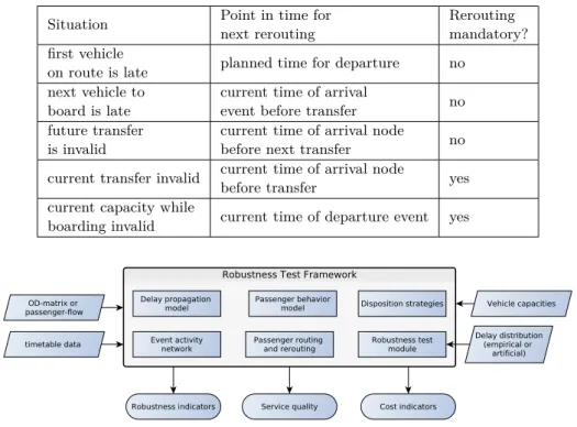
Composition of framework. The framework consists of several modules which can be instantiated in a flexible way. Figure 1 provides an overview of the overall robustness test framework, its modules and interfaces.

(6)

Table 1Classification of cases for passenger rerouting.

Situation Point in time for next rerouting

Rerouting mandatory?

first vehicle

on route is late planned time for departure no next vehicle to

board is late

current time of arrival

event before transfer no future transfer

is invalid

current time of arrival node

before next transfer no

current transfer invalid current time of arrival node

before transfer yes

current capacity while

boarding invalid current time of departure event yes

Figure 1Modules of the robustness framework.

2.2 Robustness tests

As discussed in the introduction, robustness of transport plans can be measured in many ways. In the following, we focus on small to moderate delays and take a passenger-oriented view. That means, we want to quantify the effect of delays and disturbances on passengers.

We propose the following four robustness tests.

Robustness test RT-1: Delays of single service runs (initial vehicle delay). The first robustness test considers the effect of the delay of a single service run in isolation. We evaluate many distinct scenarios, one for each service run of the given timetable. Every service run is delayed byx1minutes at its first stop. Such a delay may occur due to technical problems of some specific vehicle or due to the late arrival of some feeder vehicle causing a departing vehicle to wait for changing passengers.

Robustness test RT-2: Slow-down of single network sections (track delay). A second robustness test models scenarios where some network section invokes a certain delay. For example, temporary speed restrictions may occur because of construction work or for safety reasons. Whenever a service run passes this section, it catches a delay of x₂ minutes.

Optionally, this test can be refined by either considering bidirectional or unidirectional delays on the network section.

Robustness test RT-3: Temporary blocking of single stop (stop disruption). We model the temporary blocking of a whole stop. Such a disturbance has a starting pointtstart and a durationx3. During the blocking phase, we assume that vehicles may still enter the stop

(7)

but no vehicle can leave it. For simplicity, we further assume that the capacity to hold all vehicles at the stop is sufficient. For long-term blockings, a more detailed model would be required. When the blocking phase is over, vehicles restart from this stop one after another in the order of their scheduled departure with a constant headway ofheadwayminutes.

Robustness test RT-4: Empirical delay distributions. We use data from past observations for source delay distributions on network sections and start delays of trips. For the initial departure event of each service and for all intermediate arrival events, we draw random independent source delays from these distributions. These source delays are then propagated through the network. Since the resulting delay scenarios are randomly drawn, the tests have to be repeated many times. From several pretests we learned that 50 repetitions are sufficient to yield stable means of our test indicators in practice.

3 Experiments

In order to evaluate the proposed robustness tests, we perform a number of experiments. In this section, we will first describe the chosen test instances and how they have been generated.

Then, we discuss the choice of parameters used within the robustness tests. Then, in the main part we present the results. As indicators for robustness we use the total delay and the fraction of affected passengers. By total delay we refer to the sum of delays at their destinations experienced by all passengers across all separate parts of one robustness test.

3.1 Test data and parameters

In this paper, we use two types of instances: (1) instances based on a simplified version of the German long-distance (high-speed) train network, and (2) variations of artificial instances on a grid network as proposed in [11] for studying different planning strategies.

Construction of transport plans. Various public transport plans have been created using the LinTim-framework [13, 23]. For choosing the lines and their frequencies, a cost-based approach was chosen, see [25]. This approach starts with a line pool and assigns a frequency to each line in the pool. Lines with a frequency of zero are not chosen. The objective is to minimize the costs, i.e., to cover the demand, but using as few lines and as low frequencies as possible. From the resulting lines, we construct an event-activity network in which the timetabling step is performed. To this end, every driving, dwelling and transfer activity receives a minimum duration to which we add supplement times. To increase robustness we require for specific activities a certain minimum supplement (details below). For computing the timetable we used the fast MATCH approach introduced in [21]. After rolling out the periodic timetable for the day, a vehicle schedule is computed using a basic IP-based approach, see [6], to minimize the overall vehicle scheduling costs.

Long-distance train instances. We study four instances based on a simplified version of the German long-distance train network containing major stations in Germany and stations of neighbouring countries (Figure 2). For this network we used an artificial demand containing 380k passengers. This matches the average number of passengers travelling on long-distance trains in Germany. The four instances are based on different minimum time supplements, specified for driving sections or for dwelling activities at busy (i.e. highly used) stops:

(A) no minimum supplement times (“no_buffer”)

(B) supplement time is at least 3 minutes at busy stops (“3_min_busy_stops”)

(8)

Figure 2Long-distance train network used in this paper.

(a) Line network. (b)Travel demand.

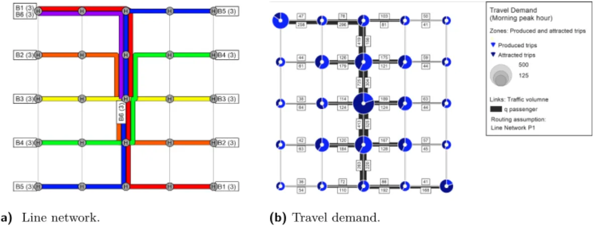
Figure 3Grid instances: Common line network of all instances with line frequencies per hour (in brackets) and the passengers’ travel demand.

(C) supplement time is at least 5% of driving time (“5_percent_drive_buffer”) (D) supplement time is at least 10% of driving time (“10_percent_drive_buffer”) Note that every periodic timetable has some intrinsic slack (due to the periodicity), i.e., usually there will be some arcs with a larger slack than the required time supplement.

Grid instances. In [12] many different line plans were tested concerning their robustness to similar tests. Based on a comparatively robust line plan (Figure 3a) we created 60 schedules that implement different strategies to distribute supplement times to further improve robustness. Figure 3b shows the travel demand (in morning peak hours) common to all instances. The demand is defined for every pair of origin and destination and every hour of the day containing 19500 passengers in total. Each vehicle is assumed to operate with a capacity of 65 passengers. All instances were created in an effort to minimize perceived travel time, number of transfers and operating costs.

Recall that we aim at studying to which extent we can increase robustness by inserting additional time supplements. With this goal in mind, we created ten different classes of instances described in Table 2. For every class we created six instances with different time supplements concerning their circulation time supplement (commonly also referred to as free layover time or supplement on turn-around). Namely, these six instances of each class

(9)

Table 2Time supplement classes for grid network.

undisturbed Class constraints for driving and dwelling times mean travel time

A no supplements 20.08 min

B 3 minutes supplements at the 5% most frequently used stops 20.19 min C 1 minute supplement for driving sections of central north-south axis 20.31 min D 2 minutes supplement for driving sections of central north-south axis 20.54 min E 3 minutes supplement for driving sections of central north-south axis 20.76 min F 3 minutes supplements at 10% most frequently used stops 20.84 min G 3 minutes supplements at 15% most frequently used stops 21.06 min H 3 minutes supplements at the 5% most frequently used driving sections 22.61 min I 3 minutes supplements at the 10% most frequently used driving sections 23.48 min J 3 minutes supplements at the 15% most frequently used driving sections 23.85 min

have at least circulation time supplements of 0,1,3,5,7 and 9 minutes. The circulation time supplement influences the vehicle schedule. The larger this supplement, the more vehicles are required. The timetable, however, remains unchanged for each instance of the same class. In Table 2, the instance classes are ordered increasingly with respect of the mean undisturbed travel times of passengers.

The operating costs of a transport plan are calculated in a simple model as the sum of two components as follows. For each used vehicle we consider the amount of travelled distance in kilometers (including empty trips) and apply a cost factor of 1.5e/km. For each used vehicle, the operating time (regular and empty trips) is multiplied with a cost factor of 50e/hwhich includes personal costs, depreciation and maintenance of the vehicle.

3.2 Setup of the robustness tests

For each robustness test, a certain range of parameters has to be chosen. We decided to vary the parameters in the following ranges.

Test RT-1: x1= 1..18 min initial vehicle delay

Test RT-2: x₂= 1..10 min delay for crossing disturbed edge Test RT-3: x₃= 10..20 min blocking time for disturbed station

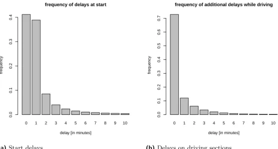
Test RT-4 applies an empirical delay distribution. We use observed delay data of German long-distance trains from a dataset of 2016-2017 containing over 28 million events for ICE and IC trains. Based on these data, we derive empirical, discrete delay distributions for two types of source delays. The first type is the starting delay of a vehicle at its first departure of a trip. The second type of delay is the additional delay of a vehicle on any driving edge (see Figures 4a and 4b). Both delay distributions are truncated to the interval between 0 and 10 minutes of delay.

Let us briefly discuss the rationale behind our parameter choices for the experiments with the grid instances. For the first test RT-1, an initial delay of more than 20 minutes would result in a simultaneous departure of the delayed vehicle and the next trip of the same line. Therefore, we choose 18 minutes as maximal delay. For experiments with the second robustness test RT-2 we choose 10 minutes as a maximum delay for a similar reason. Even larger delays would significantly decrease the number of service runs per day (unless there is enough catch-up potential). For experiments with robustness test RT-3 we choose upper

(10)

0 1 2 3 4 5 6 7 8 9 10 frequency of delays at start

delay [in minutes]

frequency 0.00.10.20.30.4

(a)Start delays.

0 1 2 3 4 5 6 7 8 9 10

frequency of additional delays while driving

delay [in minutes]

frequency 0.00.10.20.30.40.50.60.7

(b)Delays on driving sections.

Figure 4Empirical delay distributions for long-distance trains.

limits of a disruption to be 20 minutes. If the duration of the disruption is too high and every vehicle in the network passing a central station is hit by it, the propagation of delays would be too large and thus making an evaluation of resulting effects on passengers pointless.

3.3 Experiments with long-distance train network

Next we present the results of applying our robustness tests to the four instances of long- distance train networks. In a first experiment, we are interested in the impact of different delay parameters in the robustness tests RT-1 to RT-3. For robustness test RT-1, Figure 5 (left) shows the total delay of all passengers depending on different delay parametersx₁. The total delay seems to increase almost linearly with the size of the vehicle delay parameter for all instances. When we look at the results of RT-1, it seems as if there are clear differences between the four instances. Indeed, in terms of total delay instance (A) without time supplements is always worst. The slowest increase rate occurs for instance (B) with supplement times for busy stations. The ranking of the other instances changes when increasing the delay parameter. However, it is very important to note that the total delay is fairly small in absolute terms for all instances. Thus, all instances are quite robust against delays of single vehicles. Robustness tests RT-2 and RT-3 show a linear dependence on the delay parameters and yield the same ranking for all tested parameters (Figures 5 and 6). The relative gap between the instance with no time supplement and the three other instances in RT-2 (Figure 5, right) is significantly larger than in the two other experiments, and the gap is increasing with the size of the delay. For the robustness test RT-4 based on empirical delay distributions, the resulting delays for passenger routes are quite significant. We observe an average delay of 12 minutes per passenger in our instance (A) having no time supplements, about 8 minutes for instance (B), about 6 minutes for instance (C) and only 4.5 minutes for instance (D). Figure 6 (right part) shows that instance (C) has the best tradeoff between mean delay per passenger and planned travel time.

(11)

5 10 15

010002000300040005000

RT−1 − initial vehicle delay

initial delay [in minutes]

total delay [in minutes]

A − no_buffer B − 3_min_busy_stops C − 5_percent_drive_buffer D − 10_percent_drive_buffer

3 4 5 6 7 8

020000400006000080000120000

RT−2 (track delay experiment) Parameter 3−8 min

track delay [in minutes]

mean delay per disruption

Figure 5Robustness tests RT-1 and RT2 on long-distance train network.

10 12 14 16 18 20

0.0e+005.0e+061.0e+071.5e+072.0e+07

RT−3 − station disruption

station disruption duration [in minutes]

mean delay per disruption [in minutes]

152 154 156 158 160 162 164

024681012

RT−4 − empirical delays

undisturbed travel time [in minutes]

mean delay per passenger [in minutes]

A

B C

D A

B C

D A − no_buffer B − 3_min_busy_stops C − 5_percent_drive_buffer D − 10_percent_drive_buffer

Figure 6Robustness test RT-3 and RT-4 on long-distance train network. For RT-4, the stroked line is a visual guide for a linear tradeoff between undisturbed travel time and expected travel time.

0 1 2 3 4 5

46810121416

used waiting time rule [in minutes]

mean delay per passenger [in minutes]

0 1 2 3 4 5

−1.0−0.50.00.5

used waiting time rule [in minutes]

difference [in minutes]

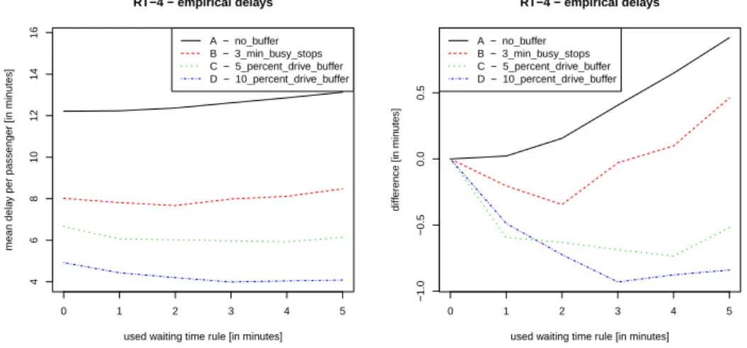
Figure 7Robustness test RT-4 on long-distance train network with different fixed waiting time rules.

(12)

Disposition strategies. The next experiment compares fixed waiting strategies for the timetables of the long-distance train network. By afixed waiting time strategy we mean the following. In case of a delayed feeder train, the departing trains waits for up toxminutes if this helps to save a planned transfer for at least one passenger. In our experiment, we compare different strategies withx∈ {0,1,2,3,4,5} wherex= 0 means NO-WAIT.

Figure 7 shows several interesting findings:

The mean delay per passenger differs significantly for instances (A)-(D): the smallest delay occurs for timetable (D) with 10% time supplement on driving sections, second best is the timetable (C) with 5% time supplement on driving sections, followed by timetable (B) with a 3-minute-supplement on busy stations. Not surprisingly, the instance (A) without extra supplement times performs worst.

The best performing fixed waiting strategy depends on the timetable. The larger the time supplements are, the longer one can afford to wait for delayed trains.

Using a fixed waiting time strategy the mean delay per passenger can be reduced by up to about 25% in comparison with NO-WAIT strategy.

3.4 Experiments with grid instances

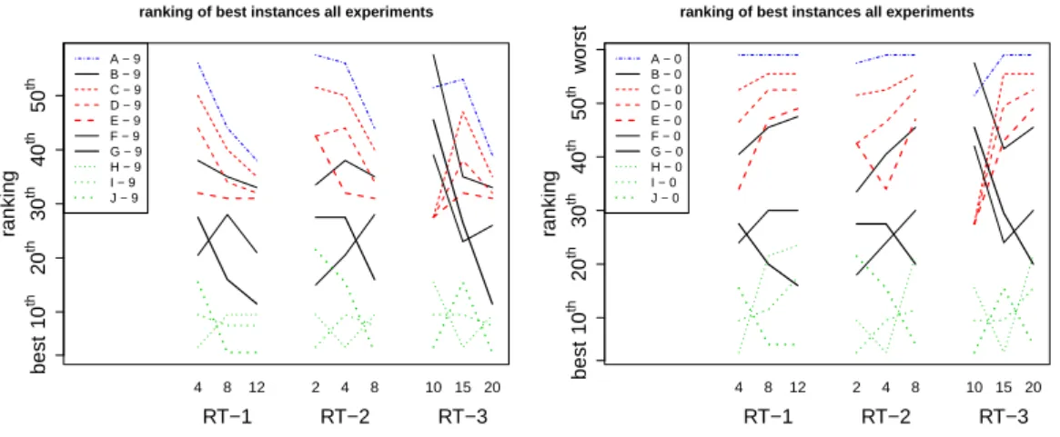
Comparison of supplement time strategies. For each of the robustness tests RT1-RT3, we obtain a ranking of the 60 grid instances with respect to the observed total delay (with rank 1 being the best). An obvious question is to ask whether we do observe different or consistent rankings for different parameters and robustness tests. If we compare the rankings of the robustness shown in Figure 8, one can see that the instances where the time supplements are placed on the driving arcs have best ranks among all classes independent from the circulation time supplement. The class of instances where the time supplements are placed at every stop rank second and the instances where the supplements are placed at the most frequently used stops rank third. We expect that circulation time supplements become more important for delay scenarios with larger delay parameters. This is confirmed in Figure 8 where rankings of instances with 9 minutes of required circulation time supplements clearly outperform those without such a required supplement. Instances with a circulation time supplement of 9 minutes in most cases improve their ranking with increasing disturbances, while instances with no circulation time supplement tend to fall off in their ranking.

Trade-off between travel time and robustness. We also have to compare the average time it takes passengers to reach their destination on an undisturbed day of traffic with the results from the robustness test. We can see this trade-off for a fixed robustness test and parameter on Figure 9 (left). Although the instances (H)-(J) have superior robustness, their tradeoff between robustness and perceived travel-time is worse than the tradeoff between the other classes of instances. In Figure 9 (right) one can see, that the costs of these solutions are significantly higher than for instances (A)-(F). These evaluations were made for one specific set of delay parameters, but tests with other sets of parameters yield similar results.

Choosing turn-around time supplements. One other question we would like to answer is:

How to choose a good turn-around time supplement? And what is the trade-off between the corresponding increased costs and reduced delays? Figure 9 can provide several insights to this question for a fixed delay parameter ofx₂= 5 minutes in RT-2. For the relatively cheap classes of schedules (A) to (F), it seems worth to invest 3 to 5 minutes of turn-around supplements.

Schedules within the class (G) to (J), however, do not require such turn-around supplements.

These schedules can already make use of other time supplements. The magnitude of regular

(13)

ranking of best instances all experiments

ranking best10th 20th 30th 40th 50th

4 8 12 2 4 8 10 15 20

RT−1 RT−2 RT−3

A − 9 B − 9 C − 9 D − 9 E − 9 F − 9 G − 9 H − 9 I − 9 J − 9

ranking of best instances all experiments

ranking best10th20th30th40th50thworst

4 8 12 2 4 8 10 15 20

RT−1 RT−2 RT−3

A − 0 B − 0 C − 0 D − 0 E − 0 F − 0 G − 0 H − 0 I − 0 J − 0

Figure 8 Comparison of timetables with respect to robustness ranking for different tests.

Instances are denoted by class (A-J) and required circulation time supplement (0 or 9 minutes).

20 21 22 23 24 25

0.00.20.40.60.81.0

RT−2 − trac delay Parameter 6 min

delay relative to maximum

0 0

00 0

0

0 0

0 9

9

99 9

9

9 9

9 B

A

CD E

F

G

H I

J

20 21 22 23 24 25

0.00.20.40.60.81.0

instance cost

instance cost relative to maximum 00 0 0 0

0 0

0 0 0

999 9 99

9 9 9

9

A C D EB F

G

H I J

Figure 9 Instances are denoted by class (A-J) and the required minimum circulation time supplement of 0 or 9 minutes. Left: We compare the robustness trade-off for all instance classes of the grid instances with respect to robustness test RT-2 with a slowdown parameter ofx2= 5 minutes. The y-axis shows the observed delay relative to the instance with maximum delay. Right:

We show the tradeoff between average undisturbed travel time (x-axis) and relative operating costs.

disruption determines the need for a turn-around time supplement. However, for small to medium disruptions the trade-off between benefit and cost for introduction of time supplements up to 3 minutes was always good for instances (A) to (F).

Three-dimensional trade-offs. We now face the challenge of evaluating transport plans to several factors simultaneously and to show their mutual trade-offs. We consider

C – operational cost,

T – average travel time of passengers, and

R – robustness measured as total delay for the passengers in our robustness tests. As combined robustness measure we take the average performance with respect to robustness tests RT1-RT3 with the delay parameters set to a medium value (RT-1 with x₁ = 8 minutes, RT-2 with x2= 5 minutes and RT-3 with x3= 15 minutes).

(14)

R

C T

(A)

R

C T

(B)

R

C T

(C)

R

C T

(D)

R

C T

(E)

R

C T

(F)

R

C T

(G)

R

C T

(H)

R

C T

(I)

R

C T

(J)

Figure 10Comparison of operational cost C, average travel-time T, and the combined robustness R with respect to robustness tests RT1-RT3 for instances (A)-(J).

5 10 15

0e+001e+052e+053e+054e+055e+05

RT−1 initial vehicle delay with circulation delay propagation

A − 0 B − 0 C − 0 D − 0 E − 0 F − 0 G − 0 H − 0 I − 0 J − 0

5 10 15

0e+001e+052e+053e+054e+055e+05

RT−1 initial vehicle delay without circulation delay propagation

A − 0 B − 0 C − 0 D − 0 E − 0 F − 0 G − 0 H − 0 I − 0 J − 0

Figure 11Comparison of robustness test RT-1 with and without vehicle circulations arcs for the grid instances.

In order to visualize the trade-off between different features we use a special form of a radar or spider chart (Figure 10). The center point of one triangle corresponds to the worst solution, while the corners represent the best value of one instance in the respective attribute. In the following comparison we concentrate on only those instances with the same circulation time supplement of 9 minutes. Instances (D), (E), (F) have a large triangle area, which can be interpreted as being good solutions over all criteria. Instance (I), however, seems to be the worst instance.

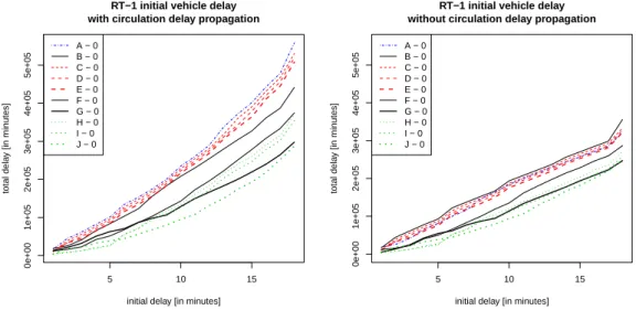
Impact of vehicle circulations. In another experiment, we studied how important it is to consider vehicle circulations. Therefore, we conducted tests with activated and deactivated vehicle circulation arcs in the EAN. As one example, we show in Figure 11 results of robustness test RT-1 with the grid instances (using zero minutes of circulation time supplement). The measured total delay is clearly significantly larger for the EAN with circulation arcs enabled than for without. It can be larger by up to a factor of 1.5. Moreover, the difference between the instance classes (A)-(J) increases with the initial delay parameter of this test. We conclude that vehicle circulation arcs should be considered.

(15)

0.0000.0100.0200.030

Capacity restriction 55−80 Instances with no circulation time supplement

maximum capacity per vehicle

fraction of affected passengers

55 60 65 70 75 80

A B C D E F G H I J

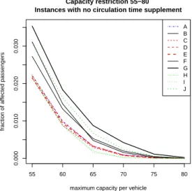
Figure 12Experiments with vehicle capacities in the range 55-80.

Impact of vehicle capacities. One important aspect covered by our model is to consider the impact of vehicle capacities in public transport. As mentioned earlier we assume hard capacities of at most 65 passengers per vehicle in our simulations. This number was used in the creation of the instances using LinTim. In the following experiment we study the dependence of experienced delays subject to different capacities. Would smaller vehicles or more passengers have an effect on our results? To answer this question we simulated undisturbed days of traffic with constant demand, and varied the maximum capacity of all vehicles. We consider the range of vehicle capacities between 55 and 80.

Figure 12 displays the fraction of passengers which for a given vehicle capacity are affected by congestion in a way that they have to adapt their planned route as they cannot board a full vehicle. We observe that for all considered timetables our assumed vehicle capacity of 65 passengers per vehicle leads to less than 1% of all passengers being affected by congestion.

Limiting the capacity further or increasing the number of passengers would decrease the robustness of the instance due to vehicle capacity constraints.

4 Summary

We have presented a general and flexible framework for performing and evaluating robustness tests with varying parameters. Extending earlier work in [12], our refined model now includes circulation arcs, vehicle capacities, a generic cost function for choosing passenger routes, and disposition strategies. Robustness tests RT1-RT3 provide public transport planners with a tool for comparing timetables without empirical delay data. By varying the delay parameters of these tests, it is possible to study the dependence of the robustness on the severeness of the delay scenario. When empirical delay data is available, the robustness test RT-4 provides realistic expected average delays. Exploring a set of instances applying different strategies for distributing time supplements, we have been able to analyze strengths and weaknesses of all instances. An interesting use case of our framework is to optimize waiting time strategies.

In future work we would like to further improve our simulations by including more information about the network infrastructure and applying sophisticated models for passenger behaviour in case of disruptions. Another extension may consider soft vehicle capacity constraints where passenger satisfaction is degraded when vehicles become too crowded.

(16)

References

1 Rodrigo Acuna-Agost, Philippe Michelon, Dominique Feillet, and Serigne Gueye. A MIP- based local search method for the railway rescheduling problem. Networks, 57(1):69–86, 2011.

2 Bastian Amberg, Boris Amberg, and Natalia Kliewer. Increasing delay-tolerance of vehicle and crew schedules in public transport by sequential, partial-integrated and integrated approaches. Procedia - Social and Behavioral Sciences, 20:292–301, 2011.

3 Bastian Amberg, Boris Amberg, and Natalia Kliewer. Robust efficiency in urban public transportation: Minimizing delay propagation in cost-efficient bus and driver schedules.

Transportation Science, 2018. doi:10.1287/trsc.2017.0757.

4 Hannah Bast, Daniel Delling, Andrew V. Goldberg, Matthias Müller-Hannemann, Thomas Pajor, Peter Sanders, Dorothea Wagner, and Renato F. Werneck. Route planning in transportation networks. In Lasse Kliemann and Peter Sanders, editors,Algorithm Engineering - Selected Results and Surveys, volume 9220 ofLecture Notes in Computer Science, pages

19–80. Springer, 2016. doi:10.1007/978-3-319-49487-6_2.

5 Nikola Bešinović, Rob M.P. Goverde, Egidio Quaglietta, and Roberto Roberti. An integrated micro-macro approach to robust railway timetabling. Transportation Research Part B: Methodological, 87:14–32, 2016.

6 Stefan Bunte and Natalia Kliewer. An overview on vehicle scheduling models. Public Transport, 1(4):299–317, 2009.

7 Serafino Cicerone, Gianlorenzo D’Angelo, Gabriele Di Stefano, Daniele Frigioni, and Al- fredo Navarra. Recoverable robust timetabling for single delay: Complexity and polynomial algorithms for special cases. Journal of Combinatorial Optimization, 18(3):229, Aug 2009.

8 Twan Dollevoet and Dennis Huisman. Fast heuristics for delay management with passenger rerouting. Public Transport, 6(1-2):67–84, 2014.

9 Twan Dollevoet, Dennis Huisman, Marie Schmidt, and Anita Schöbel. Delay management with rerouting of passengers. Transportation Science, 46(1):74–89, 2012.

10 Twan Dollevoet, Dennis Huisman, Marie Schmidt, and Anita Schöbel. Delay propagation and delay management in transportation networks. In Ralf Borndörfer, Torsten Klug, Leonardo Lamorgese, Carlo Mannino, Markus Reuther, and Thomas Schlechte, editors, Handbook of Optimization in the Railway Industry, pages 285–317. Springer International Publishing, 2018.

11 Markus Friedrich, Maximilian Hartl, Alexander Schiewe, and Anita Schöbel. Angebots- planung im öffentlichen Verkehr - planerische und algorithmische Lösungen. InHeureka’17, 2017.

12 Markus Friedrich, Matthias Müller-Hannemann, Ralf Rückert, Alexander Schiewe, and Anita Schöbel. Robustness Tests for Public Transport Planning. In Gianlorenzo D’Angelo and Twan Dollevoet, editors,17th Workshop on Algorithmic Approaches for Transportation Modelling, Optimization, and Systems (ATMOS 2017), volume 59 ofOpenAccess Series in Informatics (OASIcs), pages 6:1–6:16, Dagstuhl, Germany, 2017. Schloss Dagstuhl–Leibniz- Zentrum fuer Informatik.

13 Marc Goerigk, Michael Schachtebeck, and Anita Schöbel. Evaluating line concepts using travel times and robustness: Simulations with the LinTim toolbox.Public Transport, 5:267–

284, 2013.

14 Marc Goerigk and Anita Schöbel. An Empirical Analysis of Robustness Concepts for Timetabling. In Thomas Erlebach and Marco Lübbecke, editors, 10th Workshop on Algorithmic Approaches for Transportation Modelling, Optimization, and Systems (AT- MOS’10), volume 14 ofOpenAccess Series in Informatics (OASIcs), pages 100–113, Dag- stuhl, Germany, 2010. Schloss Dagstuhl–Leibniz-Zentrum fuer Informatik. doi:10.4230/

OASIcs.ATMOS.2010.100.

(17)

15 Géraldine Heilporn, Luigi De Giovanni, and Martine Labbé. Optimization models for the single delay management problem in public transportation. European Journal of Opera- tional Research, 189(3):762–774, 2008.

16 Sai Prashanth Josyula and Johanna Törnquist Krasemann. Passenger-oriented railway traffic re-scheduling: A review of alternative strategies utilizing passenger flow data. In7th International Conference on Railway Operations Modelling and Analysis, Lille, 2017.

17 Leo Kroon, Gábor Maróti, Mathijn Retel Helmrich, Michiel Vromans, and Rommert Dek- ker. Stochastic improvement of cyclic railway timetables. Transportation Research Part B:

Methodological, 42(6):553–570, 2008.

18 Richard M. Lusby, Jesper Larsen, and Simon Bull. A survey on robustness in railway planning. European Journal of Operational Research, 266(1):1–15, 2018.

19 Matthias Müller-Hannemann and Mathias Schnee. Efficient timetable information in the presence of delays. In R. Ahuja, R.-H. Möhring, and C. Zaroliagis, editors, Robust and Online Large-Scale Optimization, volume 5868 ofLecture Notes in Computer Science, pages 249–272. Springer, 2009.

20 Jens Parbo, Otto Anker Nielsen, and Carlo Giacomo Prato. Passenger perspectives in railway timetabling: A literature review. Transport Reviews, 36:500–526, 2016.

21 Julius Pätzold and Anita Schöbel. A Matching Approach for Periodic Timetabling. In Marc Goerigk and Renato Werneck, editors, 16th Workshop on Algorithmic Approaches for Transportation Modelling, Optimization, and Systems (ATMOS 2016), volume 54 of OpenAccess Series in Informatics (OASIcs), pages 1–15, Dagstuhl, Germany, 2016. Schloss Dagstuhl–Leibniz-Zentrum für Informatik.

22 Ralf Rückert, Martin Lemnian, Christoph Blendinger, Steffen Rechner, and Matthias Müller-Hannemann. PANDA: a software tool for improved train dispatching with focus on passenger flows. Public Transport, 9(1):307–324, 2017.

23 Alexander Schiewe, Sebastian Albert, Julius Pätzold, Philine Schiewe, Anita Schöbel, and Jochen Schulz. Lintim: An integrated environment for mathematical public transport optimization. documentation. Technical Report 2018-08, Preprint-Reihe, Institut für Numerische und Angewandte Mathematik, Georg-August Universität Göttingen, 2018.

homepage: http://lintim.math.uni-goettingen.de/.

24 Anita Schöbel. A model for the delay management problem based on mixed-integer programming. Electronic Notes in Theoretical Computer Science, 50(1), 2001.

25 Anita Schöbel. Line planning in public transportation: models and methods.OR Spectrum, 34(3):491–510, Jul 2012.

26 Anita Schöbel. An eigenmodel for iterative line planning, timetabling and vehicle scheduling in public transportation. Transportation Research Part C: Emerging Technologies, 74:348–

365, 2017.

27 Anita Schöbel and Silvia Schwarze. Finding delay-resistant line concepts using a game- theoretic approach. Netnomics, 14:95–117, 2013.

28 Peter Sels, Thijs Dewilde, Dirk Cattrysse, and Pieter Vansteenwegen. Reducing the passenger travel time in practice by the automated construction of a robust railway timetable.

Transportation Research Part B: Methodological, 84:124–156, 2016.