Robustness Tests for Public Transport Planning

(1)

Markus Friedrich

¹

, Matthias Müller-Hannemann

²

, Ralf Rückert

³

, Alexander Schiewe

⁴

, and Anita Schöbel

⁵

1 Institut für Straßen- und Verkehrswesen, Universität Stuttgart, Stuttgart, Germany

markus.friedrich@isv.uni-stuttgart.de

2 Institut für Informatik, Martin-Luther-Universität Halle-Wittenberg, Halle, Germany

muellerh@informatik.uni-halle.de

3 Institut für Informatik, Martin-Luther-Universität Halle-Wittenberg, Halle, Germany

rueckert@informatik.uni-halle.de

4 Institut für Numerische und Angewandte Mathematik, Universität Göttingen, Göttingen, Germany

a.schiewe@math.uni-goettingen.de

5 Institut für Numerische und Angewandte Mathematik, Universität Göttingen, Göttingen, Germany

schoebel@math.uni-goettingen.de

Abstract

The classical planning process in public transport planning focuses on the two criteria operating costs and quality for passengers. Quality mostly considers quantities like average travel time and number of transfers. Since public transport often suffers from delays caused by random disturbances, we are interested in adding a third dimension: robustness. We propose passenger- oriented robustness indicators for public transport networks and timetables. These robustness indicators are evaluated for several public transport plans which have been created for an artificial urban network with the same demand. The study shows that these indicators are suitable to measure the robustness of a line plan and a timetable. We explore different trade-offs between operating costs, quality (average travel time of passengers), and robustness against delays. Our results show that the proposed robustness indicators give reasonable results.

1998 ACM Subject Classification F.2.2 Nonnumerical Algorithms and Problems, G.2.2 [Graph Theory] Graph Algorithms, Network Problems)

Keywords and phrases robustness measure, timetabling, line planning, delays, passenger-orien- tation

Digital Object Identifier 10.4230/OASIcs.ATMOS.2017.6

1 Introduction

The planing process for public transport involves many stages. We here focus on the planning stage where the infrastructure (stops, available tracks or roads) is already fixed and planners are interested in the generation of apublic transport plan. By that, we mean a line network with a corresponding timetable. The primary optimization goals for public transport plans are operating costs on the one side, and quality criteria like average travel time and number

∗ This work has been partially supported by DFG grants for the research group FOR 2083.

licensed under Creative Commons License CC-BY

(2)

of transfers on the other. The effect of possible disturbances on passengers is often not considered at this stage of the planning process.

Goals and contribution. Given the same infrastructure and identical passenger demands, we aim at analyzing robustness indicators which allow for a comparison of different line plans and timetables with respect to their vulnerability to delays and disturbances. The results of the robustness test should provide planners information concerning the robustness and identify shortcomings in the line plan and timetable of the examined instance.

We propose robustness indicators which consider several types of small and large disturbances, ranging from delays for single vehicles, slow-downs of certain network sections, and temporary blockings of stops. The impacts of each test are quantified by a set of robustness indicators.

In a pilot study, we compare a set of hand-made and automatically optimized public transport plans on an artificial grid network representing an urban bus or tram network.

By comparing the characteristics of the public transport plans and the corresponding values of the robustness indicators, we aim at answering the following questions:

Are the indicators suitable to replicate the expected shortcomings of a plan?

How important is the choice of the line network for the robustness of the timetable?

Do we observe a trade-off between robustness and travel times on the basis of timetables which are optimized for the respective line plan?

Which planning method leads to more robust schedules?

Related work. Punctuality of public transport is of high importance for passengers. There- fore, a plenitude of methods exist to quantify the deviation of the realized schedule from the planned schedule. Reports often provide the percentage of services which arrive on time, wherebeing on time is defined as to arrive not later than within a given margin (e.g., 5 or 15 minutes for long distance trains) of the planned arrival time. In a Dagstuhl seminar in 2016¹, Dennis Huisman coined the phrase “passenger punctuality 2.0” for measuring the (weighted) total passenger delay at the destination for all passengers. The latter has, for example, been used by [15, 16], then also used in [10] and others. Less sophisticated indicators include the mere number of delayed departure and arrival events [4]. Alternatively, Acuna-Agost et al. [1] propose to count every time unit of delay at every planned stop and at the last stop.

Robust timetabling has been considered a lot. From an operational point of view, it is desirable that a timetable can absorb delays and recover quickly (thus avoiding penalties for the operator). To this end, inserting buffer times in the timetable may help to reduce the effect of disturbances, but may have a negative effect on the realized travel times. Not only the total amount of buffer times, but also their distribution along the lines is important. These aspects have been studied intensively in operations research. For example, Kroon et al. [11]

use stochastic optimization to allocate time supplements to make the timetable maximally robust against stochastic disturbances. They use the expected weighted delay of the trains as indicator. Using mixed integer linear programming, Sels et al. [19] improve punctuality for passenger trains in Belgium by minimizing the total passenger travel time as expected in practice. Quite recently, Bešinović et al. [3] optimized the trade-off between minimal travel times and maximal robustness using an integer linear programming formulation which includes a measure for delay recovery computed by an integrated delay propagation model in a Monte Carlo setting. In these works, the line network is usually already fixed.

1 http://www.dagstuhl.de/16171

(3)

Robustness of timetables was empirically investigated (with respect to different robustness concepts) in [8], robustness of lines has been studied in [7]. A general survey of line planning in public transport can be found in [17]. A recent integrated approach combines line planning and timetabling, but without considering robustness [18].

Overview. The remainder of this paper is structured as follows. In Section 2, we develop three different robustness tests for public transport plans. Afterwards, in Section 3, we sketch the algorithmic framework needed to compute the indicators for these tests. Then, in Section 4, we conduct an experimental study on 12 artificial public transport plans and discuss their robustness. Finally, we summarize and conclude with future work.

2 Robustness Tests

In this section, we propose three robustness tests for public transport. These robustness tests are intended to help planners in the a priori evaluation of the robustness of timetables.

With this main goal in mind, our tests shall have the following key features.

The robustness tests shall be applicable to all possible line networks and corresponding timetables in public transport and for general demand patterns varying within the course of a day.

They should capture different types of scenarios, ranging from small to more severe disturbances and occurring at different elements of the public transport plan (vehicles, network sections, stops).

They can be parameterized by severeness (how long does the disturbance take or how large are delays).

Moreover, they can also be parameterized by additional assumptions about

delay propagation and the catch-up potential of vehicles. To increase the robustness of timetables, the planned time for driving from one stop to the next or the dwelling time at stops includes some buffer time which can be used to catch-up some delay.

The catch-up potential for a delayed service, can be set by a parameterα∈R. Given for each network sectionea lower bound for the travel time`eand a planned travel time oft_e, a delayed service can reduce its delay byα·(t_e−`_e).

the disposition policy of the operating companies reacting on disturbances. For example, in an urban bus or tram network a no-wait policy might be appropriate, while in long-distance train networks certain standard waiting time rules may be used. It is also possible to use more sophisticated disposition policies by simulating the propagation of delays and the decisions of dispatchers.

In general, we take a passenger-oriented view and focus on the delay at the destination, that is, the difference between the actual arrival time and the originally planned arrival time. For measuring the impact of disturbances we distinguish four robustness indicators:

1. total delay time: the sum of all positive delays over all passengers at their destinations;

2. number of affected passengers: Every passenger arriving with a positive delay at his destination is counted as affected;

3. average delay time per affected passenger: total delay time divided by the number of affected passengers.

4. share of passengers who need to adapt their initial route: the number of passengers arriving at their destination by using a route different to the initially planned.

(4)

Disturbances may occur simultaneously at different locations or may affect subsequent runs of a vehicle schedule. To allow for a fair comparison across different line networks, different frequencies, and timetables, but fixed travel demand, the proposed indicators average over many simple scenarios with just one disturbance event. We consider three types of tests each addressing one type of disturbance. For each test, we compute the impact on the passengers, in particular, we approximate their expected delay.

Robustness test 1: Delays of single service runs. The first robustness test considers the effect of the delay of a single service run in isolation. We evaluate many distinct scenarios, one for each service run of the given timetable. Every service run is delayed byx₁ minutes at its first stop. Such a delay may occur due to technical problems of some specific vehicle or due to the late arrival of some feeder vehicle causing a departing vehicle to wait for changing passengers.

Robustness test 2: Slow-down of singe networks section. A second robustness test models scenarios where a certain network section invokes a certain delay. For example, temporary speed restrictions may occur because of construction work or for safety reasons. Whenever a service run passes this section, it catches a delay ofx2 minutes. Optionally, this index can be refined by either considering bidirectional or unidirectional delays on the section.

Robustness test 3: Temporary blocking of single stop. Finally, we model the temporary blocking of a whole stop. Such a disturbance has a starting pointt_start and a durationx₃. During the blocking phase, we assume that vehicles may still enter the stop but no vehicle can leave it. For simplicity, we further assume that the capacity to hold all vehicles at the stop is sufficient. For long-term blockings, a more detailed model would be required. When the blocking phase is over, vehicles restart from this stop one after another in the order of their scheduled departure with a constant headway ofheadwayminutes.

3 Algorithmic Framework

Next we sketch the basics of our simulation framework.

Event-activity network. A public transport timetable can be modeled as a so-calledevent- activity network (EAN) N = (V, A), i.e. a directed acyclic graph with vertex setV and arc setA. The vertices of the network correspond to the set of all arrival and departure events of the given timetable. Each event is equipped with several attributes: its type (arrival or departure), the id of the corresponding service, the stop, and several timestamps. In this context we distinguish between the planned event time according to schedule, and the realized time after the event has occurred. In an online scenario, one also has to consider the estimated event times with respect to the current delay scenario. Arcs of the network model order relations between events. We distinguish between different types of arcs (“activities”):

driving arcs, modeling the driving of a specific vehicle from one stop to its very next stop, dwelling arcs, modeling a vehicle standing at a platform and allowing passengers to enter or leave it, and

transfer arcs, modeling the possibility for passengers to change from one vehicle to another.

Every arc (activity) has an attribute which specifies its minimum duration. For driving arcs we thereby model the catch-up potential between two stops under optimal conditions. For

(5)

dwelling arcs the minimum duration corresponds to the minimum time needed for boarding and deboarding or to the setup time needed if the driving direction is changed. For transfer arcs, the minimum duration models the time which a passenger will need for the transfer.

Disposition policies. For all non-direct travelers, the effect of some delay on their arrival time at the destination depends on the chosen delay management policy of the responsible transport operator. Waiting time rules specify how long a vehicle will wait at most for a delayed feeder service. Such rules may depend on the involved lines, the time when to be applied, and other criteria. For this framework we use PANDA [14], a tool originally developed for optimized passenger-friendly disposition. This tool can be instantiated in a flexible way with almost arbitrary fixed waiting time strategies, in particular with the extreme cases of NO-WAIT and ALWAYS-WAIT.

Delay propagation. Given the source delay of some service, it will propagate from the current event to forthcoming events of the same service. Depending on the disposition policy, it may also propagate to other services. Delay propagation due to capacity restrictions of the infrastructure is not considered. New timestamps for events are derived though a propagation in breadth-first search order in the event activity network [13].

Passenger routing and rerouting. In our framework, we assume that passengers prefer to use a fastest route in their preferred starting time interval from their origin to their planned destination. Among all fastest routes they use one with the minimum number of transfers. A route is called infeasible if a transfer is missed. In our model passengers have full information about all current delays. Therefore, in the beginning of their route they do not board a vehicle if it is not on their optimal route even if they had initially planned to take this vehicle. If some intended route becomes infeasible due to delays, we assume for simplicity that passengers choose alternative routes again with the same principle (fastest routes with fewest number of transfers). Such routes can efficiently be computed by some variant of Dijkstra’s algorithm, see [2] for a recent survey on fast approaches. For large networks with many origin-destination pairs, a sufficiently fast method is needed to achieve reasonable simulation times.

Computation of robustness indicators. The computation of the proposed robustness indicators requires the following basic steps for each line plan and timetable to be evaluated:

1. Build up the event-activity network for the given line plan and timetable.

2. Compute for all groups of passengers (i.e., for all origin-destination pairs and all desired start times) optimal routes in the event-activity network and store them.

3. For each delay scenario

a.propagate the source delays through the network;

b.for each passenger group check whether the planned route is still feasible; if not, compute an alternative route;

c.evaluate the difference in arrival time for the updated route and the originally planned arrival time.

(6)

(a)Lines of P_1. (b)Lines of P_2.

Figure 1Lines of the manually created instance and their frequencies per hour (in brackets).

Figure 2Travel demand.

4 Experimental Study 4.1 Test instances

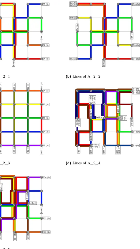
For the experiments we use the instances for line plans and timetables created in [5]. Here, an infrastructure network of 25 stops and 40 edges is considered, arranged in a grid network, see Figure 1 for two examples. All other instances are shown in the Appendix. Fig. 2 shows the travel demand (in morning peak hours) common to all instances. All instances were created in an effort to minimize travel time, number of transfers and operating costs. The impact of disturbances was neglected.

The first instances, depicted in Figure 1, are created by hand, using the experience of public transport planners. They are constructed using a system-wide frequency of 20 minutes.

(7)

A_1_1 A_1_2 A_1_3 A_1_4 A_1_5 A_2_1 A_2_2 A_2_3 A_2_4 A_2_5 P_1 P_2

average undisturbed travel time in minutes

16 17 18 19 20 21 22

(a)Average undisturbed travel time.

A_1_1 A_1_2 A_1_3 A_1_4 A_1_5 A_2_1 A_2_2 A_2_3 A_2_4 A_2_5 P_1 P_2

average transfers

0.0 0.2 0.4 0.6 0.8

(b)Average number of transfers per route.

Figure 3Quality indicators of the examined public transport plans in the undisturbed case.

The other instances contain components which are automatically generated using routines of LinTim[12, 7] where the lines and their frequencies were optimized with respect to their costs, timetables were optimized heuristically with respect to the traveling time of the passengers (using the modulo simplex in [9]) and the vehicle schedules are again optimized with respect to their costs. For a clear notation, A_x_y denotes algorithmic solutiony, based on the manual solutionP_x.

A_x_1: The lines and frequencies are fixed as in the manual plan, the timetable and vehicle schedule are automatically optimized.

A_x_2: Only the lines are fixed as in the manual plan while their frequencies, the timetable, and the vehicle schedule are automatically optimized.

A_x_3: Here only vertical and horizontal lines were allowed. Based on these lines, the line plan, the frequencies, the timetable and the vehicle schedules are automatically optimized.

A_x_4: Here, everything is calculated automatically including the line pool which is generated by the algorithm presented in [6].

A_x_5: Everything is calculated automatically, but using a combination of the manual line pool and the line pool of A_x_4.

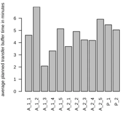
Some quality indicators of these test instances in the undisturbed planning case are shown in Figures 3 and 4. We show the average undisturbed travel time, the average number of transfers per route for the given demand, and the average transfer buffer time per transfer.

Thetransfer buffer timeis defined as the difference between the departure time of the leaving service and the arrival time of the feeder service minus the walk from the arrival to the departure platform.

4.2 Results of the robustness tests

The proposed robustness tests are applied to the grid networks. Since these instances model urban bus or tram networks, we instantiate our simulation model with a no-wait policy (as this might be most common). The parameter for the catch-up potential is set toα= 0, i.e.

it is assumed to be negligible.

(8)

A_1_1 A_1_2 A_1_3 A_1_4 A_1_5 A_2_1 A_2_2 A_2_3 A_2_4 A_2_5 P_1 P_2

average planned transfer buffer time in minutes

0 1 2 3 4 5 6

Figure 4Average transfer buffer time in minutes for the examined public transport plans in the undisturbed case.

Test 1: Delays of single service runs. We first evaluate the delay of single service runs.

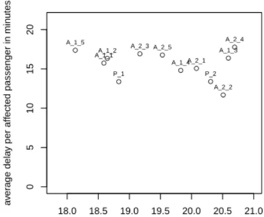
As parameter of the delay size we usex1= 10 minutes. Results are shown in Figure 5.

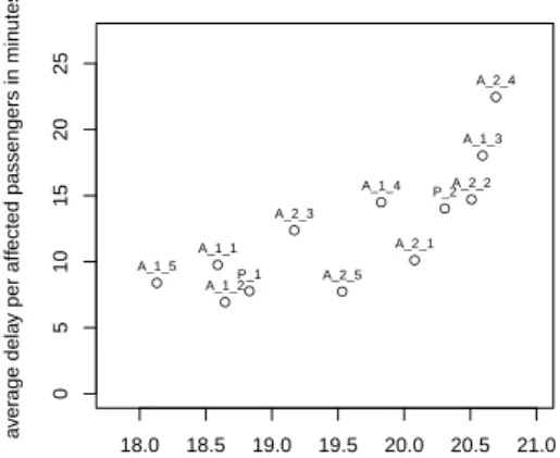
Test 2: Slow-down of single network sections. Each network section with temporary speed restrictions requires additionalx2= 3 minutes. Restrictions apply for the period of one day. Results are shown in Figure 6.

Test 3: Temporary blocking of a single stop. For the robustness indicator measuring the effect of blocked stops, we use as parameters that each stop is blocked byx3= 10 minutes.

After the restart, the required headway is assumed to be 2 minutes. As starting times of these blockings we consider every 15 minutes, giving four different scenarios for each hour.

Results are shown in Figure 7.

Discussion of results. This section interprets the robustness indicators computed above considering the form of the line network and the timetable. Table 1 summarizes the selected characteristics of the examined line networks, which can be derived directly from the network.

It also verbally lists expectations why one instance should be more or less robust. These expectations can be compared to the actual performance of each instance, which is quantified in Table 1 as the overall rank over all tests, i.e., the average rank over all three tests concerning the total delay time. Some findings of this comparison are following:

Line networks with a large number of transfer points and with lines covering many or all edges of the network provide several alternative routes for one pair of origin and destinations (OD-pair). Demand is only bundled to a small extent. Thus disturbances of one single stop affects only a relatively small amount of the demand. Demand affected by a disturbance can be diverted to alternative routes. For this reason network A_2_3 provides good results concerning the number of affected passengers and the total delay time but such a network with redundant lines comes with relative high operation costs. Line network with short line routes are less vulnerable to disturbances on single runs as one disturbance affects only few network sections. This is reflected in test 1, where most networks with short line routes perform better than networks with longer line routes. Line networks relying on one backbone line are expected to be more vulnerable. These central network elements are critical for the performance of the network making the network vulnerable if disturbances occur at single, critical network elements. Despite this expectation, most networks relying on one

(9)

Table 1Main characteristics of examined line networks influencing the robustness.

line lines lines line characteristics characteristics rank

network per per length increasing increasing test 1-3

stop edge vulnerability redundancy

one network section high frequency lines

P1, 1.7 1.5 12.0 serving as backbone, and overlapping lines 2

A_1_1 low edge coverage compensate delays 5

of other lines low service frequency

A_1_2 1.7 1.5 12.0 reduces probability of 3

being affected by short disturbances , high

transfer buffers one backbone line, short line length

A_1_3 1.2 1.0 8.0 only one transfer reduces impacts of 8

point per feeder line service run delays one network section

A_1_4 2.2 1.8 9.8 serving as backbone, 9

low edge coverage, short transfer buffer

time

A_1_5 2.5 2.2 13.9 one network section 6

serving as backbone

few OD-pairs high buffer time

P2 1,6 1.4 14.4 with alternative routes, for transfers 11

low edge coverage, long line length

few OD-pairs

A_2_1 1.6 1.4 14.4 with alternative routes, 7

low edge coverage, long line length

few OD-pairs low service frequency

A_2_2 1.6 1.4 14.4 with alternative routes, reduces probability of 10 low edge coverage, being affected by

long line length short disturbances no critical network

A_2_3 2.0 1.0 8.0 elements, all edges are 1

served by a line, short line length

A_2_4 3.4 2.4 11.1 12

long line length high frequency lines

A_2_5 2.7 1.9 15.0 increases impacts of and overlapping lines 4 service run delays compensate delays , high

transfer buffer times lines per stop: average number of lines serving a stop

lines per edge: average number of lines serving an edge

line length: average length of all line routes, weighted with service frequency overall rank: average rank over all three tests concerning the total delay time

(10)

●

● ●

●

18.0 18.5 19.0 19.5 20.0 20.5 21.0

02004006008001000

total delay per simulation in minutes

A_1_1 A_1_2

A_1_3 A_1_4

A_1_5 A_2_1

A_2_2

A_2_3

A_2_4 A_2_5

P_1

P_2

(a) Test 1: total delay per simulation in minutes.

●● ●

●

● ●

●

● ●

18.0 18.5 19.0 19.5 20.0 20.5 21.0

05101520

average delay per affected passenger in minutes

A_1_1A_1_2 A_1_3

A_1_4 A_1_5

A_2_1

A_2_2

A_2_3 A_2_4

A_2_5

P_1 P_2

(b)Test 1: average delay of affected passengers in minutes.

●

● ●

●

18.0 18.5 19.0 19.5 20.0 20.5 21.0

102030405060

# affected passengers per disruption

A_1_1 A_1_2

A_1_3 A_1_4 A_1_5

A_2_1 A_2_2

A_2_3

A_2_4 A_2_5

P_1

P_2

(c)Test 1: number of affected passengers per disruption.

●●

● ●

●

● ●

●

18.0 18.5 19.0 19.5 20.0 20.5 21.0

010203040

# of rerouted passengers

A_1_1A_1_2

A_1_3 A_1_4 A_1_5

A_2_1

A_2_2

A_2_3

A_2_4 A_2_5

P_1

P_2

(d)Test 1: number of rerouted passengers.

Figure 5Robustness indicators for Test 1: Delays of single service runs.

north-south network section as backbone (P_1, A_1_1, A1_2, A_1_5) perform better than the average. This can be explained by the setup of test 2, which slows down single network sections. The test assumes that the probability of a slow-down event does not depend on the number of lines or runs using a network section. This is not a realistic assumption. For this reason Test 2 should be modified in later tests. Service runs of overlapping lines can compensate delays of single service runs. P_1, A_1_1 and A_2_5 are examples of such a networks.

Line networks with timetables providing sufficient buffer time for transfers can compensate small or medium delays in the network. This partly explains the good performance of line network A_1_2 and A_2_5 in the case of delays on one edge. Lines with low frequencies have a lower probability of being affected by short disturbances. This effect explains the good performance of line networks A_1_2 and A_2_5 in case of disturbances at stops.

(11)

●

18.0 18.5 19.0 19.5 20.0 20.5 21.0

0100003000050000

A_1_1 A_1_2

A_1_3 A_1_4

A_1_5

A_2_1 A_2_2

A_2_3

A_2_4

A_2_5 P_1

P_2

●

18.0 18.5 19.0 19.5 20.0 20.5 21.0

0510152025

average delay per affected passengers in minutes

A_1_1 A_1_2

A_1_3

A_1_4

A_1_5

A_2_1 A_2_2 A_2_3

A_2_4

A_2_5 P_1

P_2

●●

●

● ●

●

18.0 18.5 19.0 19.5 20.0 20.5 21.0

0100200300

A_1_1A_1_2

A_1_3 A_1_4 A_1_5

A_2_1 A_2_2

A_2_3

A_2_4 A_2_5

P_1

P_2

(c) Test 2: number of affected passengers per disruption.

●

● ●

●

18.0 18.5 19.0 19.5 20.0 20.5 21.0

050001000020000

A_1_1

A_1_2

A_1_3

A_1_4

A_1_5

A_2_1 A_2_2 A_2_3

A_2_4

A_2_5 P_1

P_2

Figure 6Robustness indicators for Test 2: Slow-down of single network sections.

5 Summary and Future Work

In this paper we have proposed three robustness tests for the comparison of public transport plans. We provided a proof of concept by evaluating and comparing public transport plans for an artificial grid network. The robustness indicators showed significant differences between instances. For example, the average delay per affected passenger varies by a factor of two in Tests 2 and Test 3. Moreover, all three robustness tests are needed since they reveal different vulnerabilities.

It is well-known that the selection of the line network has a significant impact on the robustness of the corresponding public transport service. An important finding of our experiments is that the robustness tests are suitable to detect the expected shortcomings of line plans.

(12)

●

● ●

●

● ● ●

18.0 18.5 19.0 19.5 20.0 20.5 21.0

05001000150020002500

A_1_1

A_1_2

A_1_3 A_1_4

A_1_5

A_2_1 A_2_2 A_2_3

A_2_4

A_2_5

P_1 P_2

●

● ●

●

● ● ●

18.0 18.5 19.0 19.5 20.0 20.5 21.0

051015202530

average delay per affected passenger in minutes

A_1_1 A_1_2

A_1_3

A_1_4

A_1_5

A_2_1 A_2_2 A_2_3

A_2_4

A_2_5

P_1 P_2

●

18.0 18.5 19.0 19.5 20.0 20.5 21.0

708090100110

A_1_1

A_1_2

A_1_3 A_1_4

A_1_5

A_2_1 A_2_2

A_2_3

A_2_4 A_2_5

P_1

P_2

(c)Test 3: number of affected passengers per disruption.

●

● ●

●

● ●

18.0 18.5 19.0 19.5 20.0 20.5 21.0

05000100001500020000

A_1_1

A_1_2

A_1_3 A_1_4

A_1_5

A_2_1 A_2_2 A_2_3

A_2_4

A_2_5

P_1 P_2

Figure 7Robustness indicators for Test 3: Temporary blocking of a single stop.

For the three types of delay scenarios, our robustness indicators approximate the expected delay of passengers by averaging over possible disturbances as if they occur with equal probability. Clearly, if pre-knowledge is available from past observations or more detailed models about the distribution of disturbances exist, they should be used to refine the proposed indicators to weighted ones.

Future work may include several issues:

1. Can we identify hotspots where disturbances lead to a large increase in travel time?

2. For the grid networks, it has been computationally feasible to generate delay scenarios for all stops and network sections. For large scale networks, it might be necessary to use a sampling approach.

3. Do urban bus networks and long-distance train networks behave similarly?

4. What are the impacts of disturbances on the operating costs?

(13)

References

1 Rodrigo Acuna-Agost, Philippe Michelon, Dominique Feillet, and Serigne Gueye. A MIP- based local search method for the railway rescheduling problem. Networks, 57(1):69–86, 2011.

2 Hannah Bast, Daniel Delling, Andrew V. Goldberg, Matthias Müller-Hannemann, Thomas Pajor, Peter Sanders, Dorothea Wagner, and Renato F. Werneck. Route planning in transportation networks. In Lasse Kliemann and Peter Sanders, editors,Algorithm Engineering – Selected Results and Surveys, volume 9220 of Lecture Notes in Computer Science, pages

19–80. Springer, 2016. doi:10.1007/978-3-319-49487-6_2.

3 Nikola Bešinović, Rob M.P. Goverde, Egidio Quaglietta, and Roberto Roberti. An integrated micro-macro approach to robust railway timetabling. Transportation Research Part B: Methodological, 87:14–32, 2016.

4 Serafino Cicerone, Gianlorenzo D’Angelo, Gabriele Di Stefano, Daniele Frigioni, and Al- fredo Navarra. Recoverable robust timetabling for single delay: Complexity and polynomial algorithms for special cases. Journal of Combinatorial Optimization, 18(3):229, Aug 2009.

5 Markus Friedrich, Maximilian Hartl, Alexander Schiewe, and Anita Schöbel. Angebots- planung im öffentlichen Verkehr – planerische und algorithmische Lösungen. InHeureka’17, 2017.

6 Philine Gattermann, Jonas Harbering, and Anita Schöbel. Line pool generation. Public Transport, 9:7–32, 2017.

7 Marc Goerigk, Michael Schachtebeck, and Anita Schöbel. Evaluating line concepts using travel times and robustness: Simulations with the lintim toolbox. Public Transport, 5(3):267–284, 2013.

8 Marc Goerigk and Anita Schöbel. An empirical analysis of robustness concepts for timetabling. In Proceedings of ATMOS10, volume 14 of OpenAccess Series in Informatics (OASIcs), pages 100–113, Dagstuhl, Germany, 2010.

9 Marc Goerigk and Anita Schöbel. Improving the modulo simplex algorithm for large-scale periodic timetabling. Computers and Operations Research, 40(5):1363–1370, 2013.

10 Géraldine Heilporn, Luigi De Giovanni, and Martine Labbé. Optimization models for the single delay management problem in public transportation. European Journal of Opera- tional Research, 189(3):762–774, 2008.

11 Leo Kroon, Gábor Maróti, Mathijn Retel Helmrich, Michiel Vromans, and Rommert Dek- ker. Stochastic improvement of cyclic railway timetables. Transportation Research Part B:

Methodological, 42(6):553–570, 2008.

12 LinTim – Integrated Optimization in Public Transportation. Homepage. see http://

lintim.math.uni-goettingen.de/.

13 Matthias Müller-Hannemann and Mathias Schnee. Efficient timetable information in the presence of delays. In R. Ahuja, R.-H. Möhring, and C. Zaroliagis, editors, Robust and Online Large-Scale Optimization, volume 5868 ofLecture Notes in Computer Science, pages 249–272. Springer, 2009.

14 Ralf Rückert, Martin Lemnian, Christoph Blendinger, Steffen Rechner, and Matthias Müller-Hannemann. PANDA: a software tool for improved train dispatching with focus on passenger flow. Public Transportation, 2016. DOI 10.1007/s12469-016-0140-0.

15 Anita Schöbel. A model for the delay management problem based on mixed-integer programming. Electronic Notes in Theoretical Computer Science, 50(1), 2001.

16 Anita Schöbel.Optimization in public transportation. Stop location, delay management and tariff planning from a customer-oriented point of view. Optimization and Its Applications.

Springer, New York, 2006.

17 Anita Schöbel. Line planning in public transportation: models and methods.OR Spectrum, 34(3):491–510, Jul 2012.

(14)

18 Anita Schöbel. An eigenmodel for iterative line planning, timetabling and vehicle scheduling in public transportation. Transportation Research Part C: Emerging Technologies, 74:348–

365, 2017.

19 Peter Sels, Thijs Dewilde, Dirk Cattrysse, and Pieter Vansteenwegen. Reducing the passenger travel time in practice by the automated construction of a robust railway timetable.

Transportation Research Part B: Methodological, 84:124–156, 2016.

(15)