Environmental Policy and the Macroeconomy in the Presence of Ecological Thresholds

IHS Economics Series Working Paper 269

May 2011

Environmental Policy and the Macroeconomy in the Presence of Ecological Thresholds

Ben J. Heijdra

Pim Heijnen

Impressum Author(s):

Ben J. Heijdra, Pim Heijnen Title:

Environmental Policy and the Macroeconomy in the Presence of Ecological Thresholds ISSN: Unspecified

2011 Institut für Höhere Studien - Institute for Advanced Studies (IHS) Josefstädter Straße 39, A-1080 Wien

E-Mail: o ce@ihs.ac.atffi Web: ww w .ihs.ac. a t

All IHS Working Papers are available online: http://irihs. ihs. ac.at/view/ihs_series/

This paper is available for download without charge at:

https://irihs.ihs.ac.at/id/eprint/2060/

Environmental Policy and the Macroeconomy in the Presence of Ecological Thresholds

Ben J. Heijdra, Pim Heijnen

269

Reihe Ökonomie

Economics Series

269 Reihe Ökonomie Economics Series

Environmental Policy and the Macroeconomy in the Presence of Ecological Thresholds

Ben J. Heijdra, Pim Heijnen May 2011

Institut für Höhere Studien (IHS), Wien

Institute for Advanced Studies, Vienna

Contact:

Ben J. Heijdra

Faculty of Economics and Business University of Groningen

P.O. Box 800

9700 AV Groningen, The Netherlands

: +31/50/363-7303 Fax: +31/50/363-7337 email: info@heijdra.org and

Institute for Advanced Studies, CESifo, Netspar Pim Heijnen

Faculty of Economics and Business University of Groningen

P. O. Box 800

9700 AV Groningen, The Netherlands

: +31/50/363-3789 Fax: +31-50-363-7337 email: p.heijnen@rug.nl

Founded in 1963 by two prominent Austrians living in exile – the sociologist Paul F. Lazarsfeld and the economist Oskar Morgenstern – with the financial support from the Ford Foundation, the Austrian Federal Ministry of Education and the City of Vienna, the Institute for Advanced Studies (IHS) is the first institution for postgraduate education and research in economics and the social sciences in Austria. The Economics Series presents research done at the Department of Economics and Finance and aims to share “work in progress” in a timely way before formal publication. As usual, authors bear full responsibility for the content of their contributions.

Das Institut für Höhere Studien (IHS) wurde im Jahr 1963 von zwei prominenten Exilösterreichern – dem Soziologen Paul F. Lazarsfeld und dem Ökonomen Oskar Morgenstern – mit Hilfe der Ford- Stiftung, des Österreichischen Bundesministeriums für Unterricht und der Stadt Wien gegründet und ist somit die erste nachuniversitäre Lehr- und Forschungsstätte für die Sozial- und Wirtschafts- wissenschaften in Österreich. Die Reihe Ökonomie bietet Einblick in die Forschungsarbeit der Abteilung für Ökonomie und Finanzwirtschaft und verfolgt das Ziel, abteilungsinterne Diskussionsbeiträge einer breiteren fachinternen Öffentlichkeit zugänglich zu machen. Die inhaltliche Verantwortung für die veröffentlichten Beiträge liegt bei den Autoren und Autorinnen.

Abstract

We study the environmental and economic effects of public abatement in the presence of multiple stable steady-state ecological equilibria. Under shallow-lake dynamics (SLD), the isocline for the stock of pollution features two stable branches, a good and a bad one.

Assuming that the ecology is initially located on the upper (bad) branch of the isocline, the ecological equilibrium is hysteretic and a suitably designed temporary abatement policy can be used to steer the environment from the bad to the good equilibrium. In all models considered in this paper, a “cold turkey” abatement policy is optimal, i.e. the largest feasible shock should be administered for the shortest possible amount of time. Depending on the particular model used to characterize the economic system, there is a capital feedback effect that either helps or hinders the attainment of a successful abatement policy.

Keywords

Shallow-lake dynamics, bifurcation, environmental policy, abatement, overlapping generations

JEL Classification

D60, E62, H23, H63, Q20, Q28, Q50

Comments

We thank various participants at the macro breakfast seminar (IHS Wien), the TU Wien, the EEA 2010 meetings (University of Glasgow), and the 2010 GAM Workshop (University of Warwick).

Contents

1 Introduction 1

2 Core model 3

2.1 Ecological system ... 3

2.2 Economic system ... 6

2.2.1 Households ... 6

2.2.2 Firms ... 7

2.2.3 Equilibrium ... 9

3 Environmental and macroeconomic effects of public abatement 10 4 Extensions 16

4.1 Endogenous labour supply ... 17

4.2 Finite lives ... 21

5 Conclusions 27 Appendix: Welfare analysis 28

A First-best social optimum ... 28

B Second-best social optimum ... 31

C Equivalent-variation welfare measure for the BY model ... 36

References 36

1 Introduction

In this paper we revisit an important theme in environmental macroeconomics, namely the environmental and economic effects of public abatement activities. The existing literature typically studies environmental policy with the aid of “linear models” in which gradual changes in dirt emissions have gradual effects on the ecological system – Bovenberg and Heijdra (1998, 2002) are examples of this approach.

In recent years, however, prominent ecologists have argued that in many cases nature does not respond smoothly to gradual changes at all (e.g. Arrow et al. 1995). Scheffer et al. (2001) postulate the key elements of this new view. First, ecosystems do not respond smoothly to gradual changes in dirt flows, abrupt “catastrophic shifts” may be possible in the vicinity of threshold points, and there are typically no early warning signals for such shifts.

¹

Second, there may be multiple stable equilibria. Third, irreversibility and hysteresis are all possible.

The prototypical example of the phenomenon under consideration concerns shallow lakes:

One of the best-studied and most dramatic state shifts is the sudden loss of trans- parency and vegetation observed in shallow lakes subject to human-induced eu- trophication. The pristine state of most shallow lakes is probably one of clear water and a rich submerged vegetation. Nutrient loading has changed this situa- tion in many cases. Remarkably, water clarity often seems to be hardly affected by increased nutrient concentration until a critical threshold is passed, at which the lake shifts abruptly from clear to turbid. With this increase in turbidity, sub- merged plants largely disappear. Associated loss of animal diversity and reduction of the high algal biomass makes this state undesired. Reduction of nutrient con- centrations is often insufficient to restore the vegetated clear state. Indeed, the restoration of clear water happens at substantially lower nutrient levels than those at which the collapse of the vegetation occurred (Scheffer et al., 2001, p. 592).

The nonlinear ecological dynamics described by Scheffer et al. (2001) now carries the name Shallow-Lake Dynamics (SLD hereafter).

²

But the same phenomenon holds for a range of

1There is an emerging literature on early warning systems. See Biggs et al. (2009).

2For overviews of the SLD approach, see Muradian (2001), M¨aleret al.(2003), Brock and Starrett (2003), and Wagener (2009). For economic applications of SLD, see Heijnen and Wagener (2009), Ranjan and Shortle (2007), and Wirl (2004). A related nonlinear approach is used by Prieur (2009).

other ecological systems such as coral reefs, boreal forests, savannas and grasslands, and seas.

³

Ecological systems featuring thresholds and flip points appear to be the rule rather than the exception. Indeed, there now exist several websites with databases documenting a broad variety of cases.

⁴

The objective of this paper is to study the effects of public abatement on the environment and the economic system when the ecological system features SLD. We have chosen to focus on SLD not because we think that the ecology literally behaves just like a shallow lake but rather because SLD provides a simple and tractable framework in which there are potentially multiple stable steady states.

⁵

The specific scenario that we study thus has the following key features. First, we assume that the flow of dirt is such that there exist two stable ecological steady-state equilibria. Second, we postulate that the ecological system has settled down at the “bad” equilibrium featuring a high stock of pollution.

⁶

In this setting we consider which kind of abatement policy the policy maker should conduct in order to clean up the environment and to move the ecological equilibrium from the bad to the good steady state.

Our mode of attack is as follows. To study the economic effects of abatement, we develop a basic representative-agent model of a closed economy. Households practice intertemporal consumption smoothing and accumulate capital that is rented out to perfectly competitive firms. Following Bovenberg and Heijdra (2002), we assume that the capital stock is the pol- luting production factor. Households enjoy living in a clean environment but act as free riders and thus fail to internalize the external effects caused by their capital accumulation decisions.

As a result, there is a meaningful role for the policy maker. By restricting attention to abate- ment, we implicitly assume that the policy maker has a fairly restrictive set of instruments to conduct its environmental policy. Indeed, as we argue in the paper, the first-best social

3See, for example, M¨aler and Li (2010), Cr´epin (2007), Janssen, Anderies, and Walker (2004), and Cr´epin (2003).

4See the threshold databases of the Resilience Alliance (www.resalliance.org) and the Stockholm Re- silience Centre (www.stockholmresilience.org). Arrowet al. (1995, p. 521) define resilience as “a measure of the magnitude of disturbances that can be absorbed before a system centered on one locally stable equilib- rium flips to another.”

5For a survey on ecosystem dynamics, see Levin and Pacala (2003). They briefly discuss SLD on pages 79-80. In future work we will study alternative specifications for the ecological system. We believe our main results to be quite robust.

6In the context of our model this sorry state of affairs could have arisen if the capital stock was much more polluting in the past than it is at present.

optimum calls for a positive capital tax, but this Pigouvian instrument is not available by assumption. A temporary abatement policy can nevertheless be successful in steering the ecological equilibrium from the bad to the good steady state, thus increasing welfare of the representative agent.

The rest of the paper is structured as follows. Section 2 presents the core model, con- sisting of an ecological system featuring SLD and an economic system. Section 3 studies the environmental and macroeconomic effects of a stepwise temporary abatement shock. We analytically characterize the qualitative effects at impact, during transition, and in the long run. To visualize and quantify these effects we also develop a plausibly calibrated version of the model. The model features a trade-off between shock size and shock duration. Given the form of the dirt flow equation, the best abatement policy in the class of stepwise shocks is a

“cold turkey” policy, i.e. the maximum feasible shock for the shortest possible duration. In Section 4 we study some extensions to the model. The first extension endogenizes the rep- resentative household’s labour supply decision. This makes abatement policy more difficult because labour supply and the capital stock (and thus pollution) expand during transition as a result of the additional taxes needed to finance the abatement spending. The second extension assumes that the economy is populated by overlapping generations of finite-lived agents. In this setting abatement policy becomes easier because the tax increases leads to capital crowing out (and reduced pollution) during transition. In both extensions the cold turkey result continues to hold. Finally, in Section 5 we offer a brief summary of the main results, whilst the Appendix presents some details of the welfare analysis.

2 Core model

2.1 Ecological system

The environment is modelled as a renewable resource stock. Its quality depends negatively on the flow of dirt, D (t), that is generated in the production process:

D (t) ≡ κK(t) − γG(t), κ > 0, γ > 0, (1)

where K (t) is the private capital stock (see below), and G (t) represents abatement activities

by the government. Capital is assumed to be the polluting factor of production, just as in

Bovenberg and Heijdra (1998, 2002).

⁷

By definition the flow of dirt must be non-negative (D (t) ≥ 0).

⁸

Denoting the stock of pollution at time t by P (t), we write the general form of the emission equation as:

P ˙ (t) = −πP (t) + P (t)

²

P (t)

²

+ 1 + D (t) , π > 1

2 , (2)

where ˙ P (t) ≡ dP (t) /dt. The first term on the right-hand side shows that nature features a regenerative capacity (since π > 0), whilst the second term represents the shallow-lake dynamics (SLD) – see M¨ aler et al. (2003, p. 606).

We assume that π >

¹₂

, thus ensuring that nature does not feature irreversible equilibria.

To see why this is the case, consider Figure 1 depicting the phase diagram for the stock of pollution. The ˙ P (t) = 0 line is obtained from (2) and represents all combinations of P (t) and D (t) such that the stock of pollution is constant over time. With π >

¹₂

the ˙ P (t) = 0 line is S-shaped, with threshold points at D (t) = D

L

and D (t) = D

U

.

⁹

The vertical arrows depict the dynamic forces operating on the stock of pollution off the ˙ P (t) = 0 line.

For time-invariant dirt flows satisfying 0 ≤ D < D

L

and D > D

U

, there is a unique and stable ecological steady state to which nature converges. In contrast, for D

L

≤ D ≤ D

U

there exist two stable ecological steady-state equilibria, i.e. the lower branch (through points C

^′

, A, and B) and the upper branch (from point C to point D and beyond) are both stable.

¹⁰

Which particular steady state is attained depends on initial conditions, i.e. the ecological

7Xepapadeas (2005, p. 1239) proposes a more general functional form of the type D(t) = Φ (K(t), G(t)) with∂Φ/∂K(t)>0 and∂Φ/∂G(t)<0. We have chosen a linear form for convenience and because it allows us to zero in on the nonlinear features due to SLD.

8We interpretD(t) as thenetdirt flow which must be non-negative by definition. Initiatives such as Carbon Capture and Storage (CCS) can be seen as a way to increase the value of π in the ecological function (2).

Since CCS is rather ineffective at present, we ignore this mechanism in this paper.

9These points are implicitly defined. TheP-coordinates of points B and C in Figure 1 are the solutions to:

φ(π, P)≡ −π

2+ P

(1 +P²)² = 0.

The funtionφ(π, P) is the derivative with respect toPof the right-hand side of (2). The zeroes of this function are associated with one local minimum dirt flow and one local maximum dirt flow. These dirt flow thresholds are themselves obtained by substituting these coordinates into (2) and imposing ˙P(t) = 0. Forπ= 1/2, we find PL= 1 andDL= 0, i.e. point C is on the vertical axis and the ecology featuresirreversible equilibria, namely all steady-state points located on the upper branch of the ˙P(t) = 0 line. Since the flow of dirt cannot become negative, there is no way to get to the lower branch from there.

10The branch connecting points B and C is unstable, i.e. all vertical arrows point away from it.

model features hysteresis. An economy which starts out with a relatively low dirt flow will find itself on the lower branch. Even a sizeable increase in the dirt flow will only result in a small increase in the steady-state stock of pollution – see for example the move from point C

^′

to A. An economy which lets things get too dirty, however, and produces a dirt flow exceeding the upper threshold (D (t) > D

_U

) will experience a catastrophic increase in the pollution stock and end up on the upper branch of the ˙ P (t) = 0 line, say at point B

^′

. A subsequent reduction in the dirt flow will move the ecological steady-state along the upper branch, say from point B

^′

to point D. Even though the dirt flow is the same in the dirty equilibrium D and in the clean equilibrium A, D (t) = ˆ D

₀

, the stock of pollution is much higher in the dirty equilibrium, i.e. ˆ P

B

> P ˆ

G

. To make things worse, there is no way to get from D to A without reducing the dirt flow below its lower threshold value for a long enough period of time.

In a qualitative sense, to get from point D to point A, the following road must be traveled.

First, the dirt flow should be set such that D (t) < D

L

. In Figure 1 this produces, say, the shift from point D to D

₁

. This point lies in the basin of attraction of the lower branch of the P ˙ (t) = 0 line as the vertical arrows indicate. Abstracting from economic feed-back effects (see below), the ecology moves in the direction of points C

₁

and E

₁

. Second, the stock of pollution must be allowed to fall below a critical level, P

E

, representing the stock associated with point E in the figure. Third, once the ecology has passed point E

₁

, the dirt flow must be restored to its initial level ˆ D

0

. Since P (t) < P

E

, the ecology will ultimately converge to point A.

But this is the mechanical story associated with SLD. As is shown in equation (1), the

flow of dirt depends in part on the abatement activities of the government but also on the

macroeconomic capital stock, i.e. on the savings behaviour of the economic agents in the

economy. And to make things worse, the resources needed by the government to conduct

its abatement activities will in general affect the behaviour of these very agents, i.e. K (t)

is not independent from G (t). In the next subsection a simple general equilibrium model is

postulated to capture this dependency.

P(t) = 0 .

P ˆ

G

!

A

B C

!

!

!

D(t) / 6 K(t) ! (G(t) D

C N

!

B N

!

D

_L

D

_U

P(t)

P ˆ

B

D ˆ

₀

! E P

E

!

! D

1

E

1

! C

₁

P

L

P

_U

Figure 1: Ecological dynamics 2.2 Economic system

In this subsection we formulate a simple general equilibrium model of the macroeconomy.

¹¹

This core model describes a closed economy and is populated by representative households and firms who are blessed with perfect foresight.

2.2.1 Households

The representative household lives forever, and features the following utility functional:

Λ(t) ≡ Z

∞

t

h ln C(τ ) + ε

_E

ln E ¯ − P (τ ) i

· e

^ρ(t−τ)

dτ , (3)

where C(τ ) denotes consumption of private commodities at time τ , E (τ ) ≡ E ¯ − P (τ ) > 0 measures the quality of the environment, ¯ E is some pristine value attained in a non-polluting society, ε

E

denotes the weight in overall utility attached to environmental amenities, and ρ ≥ 0 stands for the pure rate of time preference. Since utility is separable in its two arguments, the quality of the environment does not directly affect household consumption. Since the felicity

11Our discussion of the standard economic models used in this paper is quite compact. For a textbook treatment of these models, see for example Heijdra (2009).

function for private consumption is logarithmic, the model features a unitary intertemporal elasticity of substitution.

¹²

Without leisure entering utility, labour supply is exogenously fixed (but see subsection 4.1 below).

Households face the following budget identity:

A ˙ (τ ) = r(τ )A(τ ) + w(τ ) − T (τ ) − C(τ ), (4) where r(τ ) denotes the real rate of interest on financial assets, w(τ ) represents the wage rate, T (τ ) are net lump-sum taxes, and A(τ ) stands for real financial assets owned in period τ . As usual we define ˙ A (τ ) ≡ dA(τ )/dτ.

The representative agent chooses paths for C(τ ) and A (τ ) which maximize (3) subject to (4) and a solvency requirement. The solution for consumption at time t amounts to:

C(t) = ρ · [A(t) + H(t)], (5)

where human wealth, H(t), is given by:

H(t) ≡ Z

∞

t

[w(τ ) − T (τ )] · e

^{−Rtτr(s)ds}

dτ . (6)

The optimal time profile for consumption is given by the Euler equation:

C ˙ (τ )

C (τ ) = r (τ ) − ρ, τ ≥ t. (7)

Equation (5) shows that the agent consumes a constant proportion of total wealth in the planning period, whilst equation (7) shows that consumption growth over time is chosen to be equal to the rationally anticipated gap between the interest rate and the rate of time preference. Finally, the expression in (6) shows that human wealth is given by the discounted value of after-tax wage payments. Intuitively it thus represents the after-tax value of the agent’s unitary time endowment.

2.2.2 Firms

The production sector of the economy is perfectly competitive. The production function is Cobb-Douglas, with constant returns to scale to the factors capital, K(t), and labour, L(t):

Y (t) ≡ F (K(t), L(t)) = Ω

0

K(t)

^εL

L(t)

^1−εL

, Ω

0

> 0, 0 < ε

L

< 1, (8)

12We adopt simple functional forms for felicity and production functions in order to keep our economic analysis as simple as possible. By adopting this approach we are better able to zoom in on the complications arising from the nonlinear environmental dynamics.

Table 1: The core model

C(t) ˙

C (t) = r(t) − ρ, ρ > 0 (T1.1)

K(t) = ˙ Y (t) − C(t) − G (t) − δK(t) (T1.2)

[r(t) + δ] K(t) = (1 − ε

L

)Y (t) (T1.3)

w(t)L(t) = ε

L

Y (t) (T1.4)

Y (t) = Ω

0

L(t)

^εL

K(t)

^1−εL

, Ω

0

> 0, 0 < ε

L

< 1 (T1.5)

L(t) = 1 (T1.6)

P ˙ (t) = −πP (t) + P (t)

²

P (t)

²

+ 1 + D(t), π > 1

2 (T1.7)

D(t) = κK (t) − γG(t), κ > 0, γ > 0 (T1.8)

Endogenous: consumption, C(t), capital stock, K(t), output, Y (t), interest rate, r(t), wage rate, w(t), employment, L(t), pollution stock, P(t), dirt flow, D(t). Exogenous: govern- ment abatement, G(t). Parameters: rate of time preference, ρ, depreciation rate of capital, δ, labour coefficient in the technology, ε_L, and scale factor in the technology, Ω0. Ecological pa- rameters: lake resilience, π, capital dirt coefficient, κ, and abatement clean-up coefficient, γ.

where Y (t) denotes gross output. The representative firm maximizes the value of the firm, V (t), which is defined as follows:

V (t) = Z

∞

t

[Y (τ ) − w(τ )L(τ ) − I(τ )] · e

^{−Rtτr(s)ds}

dτ , (9) subject to the production function, and the capital accumulation identity:

K ˙ (τ ) = I (τ ) − δK (τ ) , (10)

where ˙ K(τ ) ≡ dK(τ )/dτ denotes the rate of change in the capital stock and δ is the deprecia- tion rate (δ > 0). The first-order conditions for value maximization imply the usual marginal productivity conditions:

∂Y (τ )

∂K (τ ) = r(τ ) + δ, ∂Y (τ )

∂L(τ ) = w(τ ). (11)

K(t) E

₀

K ˆ

C(t)

(K(t) = 0) .

₀

C(t) = 0 .

K ˆ

^GR

A

!

! E

^GR

!

!

! B

(K(t) = 0) .

₁

E

₁

! C ˆ

C(0)

SP

₀

Figure 2: Consumption-capital dynamics in the core model

Since we abstract from adjustment costs in investment, the value of equity corresponds to the replacement value of the capital stock, i.e. V (t) = K(t).

2.2.3 Equilibrium

For convenience, the key equations of the core model have been gathered in Table 1. Equation (T1.1) is the Euler equation (7), whilst equations (T1.5) and (T1.7)–(T1.8) just restate, respectively (8), (2), and (1). Labour supply is exogenous so L (t) = 1 – see (T1.6). The factor demand expressions in (11) have been rewritten by using the production function – see (T1.3) and (T1.4). Equation (T1.2) is obtained by combining (10) with the goods market clearing condition for a closed economy, i.e. Y (τ ) = C (τ ) + I (τ ) + G (τ ). Finally, in the absence of government debt, claims on the capital stock are the only assets available, i.e.

A (t) = K (t).

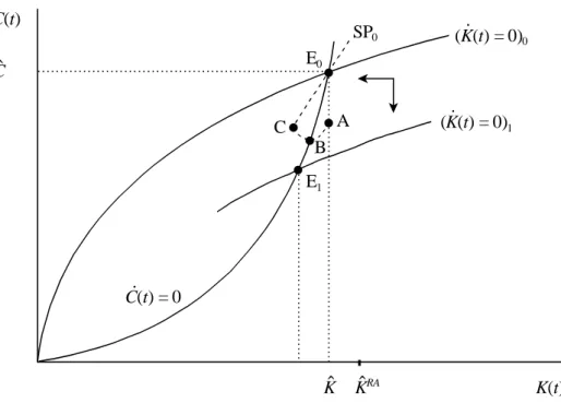
The phase diagram for the economic system is depicted in Figure 2.

¹³

The initial equilib-

13Note that the economy influences the ecology but not vice versa. Hence, even though the full model is

rium, by assumption featuring no public abatement, is at point E

₀

. Steady-state consumption and the capital stock are given by, respectively, ˆ C and ˆ K. The equilibrium is saddle-point stable, with SP

₀

representing the saddle path, and is dynamically efficient, i.e. ˆ K is strictly less than the golden-rule capital stock, ˆ K

^GR

.

3 Environmental and macroeconomic effects of public abate- ment

In this section we study the effects of public abatement on the environment, the macroecon- omy, and on individual welfare. Much of the existing literature on environmental macroeco- nomics only looks at “regular”, non-hysteretic, ecological systems – see for example Bovenberg and Heijdra (1998, 2002) and the references therein. In essence this literature assumes that the ˙ P (t) = 0 curve is monotonically increasing, rather than S-shaped. In such a setting, the policy maker must engage in a permanent abatement policy in order to attain a par- ticular welfare maximizing point on the ˙ P (t) = 0 curve. Because the ecological system is non-hysteretic, a temporary abatement policy cannot be used.

In stark contrast, as was argued above in our intuitive discussion of Figure 1, in the presence of SLD the ecological system is hysteretic, and there may be two welfare-rankable equilibria, namely a clean and a dirty one. Furthermore, a suitably designed temporary abatement policy can be used to shift the environment from the dirty to the clean equilibrium.

Assume that the economy is initially at the steady-state equilibrium (point E

₀

in Figure 2) and that the ecological equilibrium is at point D in Figure 1. Since G (t) = 0 initially, the dirt flow associated with point D is equal to ˆ D

₀

= κ K. At this dirt flow there is another stable ˆ equilibrium at point A in Figure 1 which, from a steady-state perspective, features a higher level of welfare.

In order to move the ecological equilibrium from point D to point A, we assume that the policy maker engages in an abatement policy of the following type:

G (t) =







G for 0 ≤ t ≤ t

E

0 for t > t

E

(12)

characterized by a three-dimensional system of nonlinear differential equations, the recursivity of this system allows us to use simple two-dimensional phase diagrams such as Figures 1 and 2.

where the shock is administered at time t = 0, t

_E

represents the duration of the shock, and G is its size. Figure 2 shows the qualitative nature of the adjustment paths of consumption and the capital stock. The abatement shock shifts the ˙ K (t) = 0 line down as less resources are available for private consumption and investment. If the shock were permanent (t

E

→ ∞), the equilibrium would instantaneously shift from E

₀

to E

₁

, i.e. the economy would feature a once off reduction in private consumption. Provided G is sufficiently large such that 0 ≤ κ K ˆ − γG < D

_L

, the ecology would gradually move to the lower branch of the ˙ P (t) = 0 line in Figure 1. It would reach a steady state to the left of point C

^′

.

To reach point A from D a temporary policy (0 < t

_E

< ∞) is needed. In terms of Figure 2, such a shock produces the adjustment path from A through B to E

₀

. At impact (t = 0) the capital stock is predetermined and the economy shifts from point E

₀

to A. The increased tax bill leads to an immediate reduction in human wealth and thus causes agents to cut back consumption – see (5) and (6) above.

¹⁴

At point A, the dynamic forces are those indicated by the north-west arrows and for 0 < t < t

_E

the economy gradually moves from A to B. During transition the capital stock falls short of its steady-state level (K (t) < K), the interest rate exceeds the rate of time ˆ preference (r (t) > ρ), and the optimal consumption profile is upward sloping – see (7) above.

Also, since the economy is located above the then relevant ˙ K (t) = 0 line, there is too little investment and the capital stock falls over time. Point B is reached at time t

E

, at which moment the ˙ K (t) = 0 curve shifts back to its original position. The resources previously used for abatement can once again be used to restore the capital stock and consumption to their original levels.

The flow of dirt during the abatement policy features two jumps (namely at times t = 0 and t = t

E

), is downward sloping for 0 < t < t

E

, and is upward sloping for t ≥ t

E

. Interestingly, the policy shock prompts a reaction from the private sector in the form of a temporarily lower capital stock which boosts the environmental cleanup.

Of course, not just any temporary policy will result in a successful transition from point

14Taxes and government spending are related to each other via the intertemporal government budget con- straint. In the absence of government debt at timet, this constraint is given by:

0≡ Z ∞

t

[T(τ)−G(τ)]·e^{−Rtτr(s)ds}dτ .

Table 2: Structural parameters and steady-state features

Economic system:

ρ = 0.04 δ = 0.07 ε

L

= 0.70 Ω

₀

= 0.7401 ˆ

r = 0.04 K ˆ = 2.7273 Y ˆ = 1.000 C ˆ = 0.8091 I ˆ = 0.1909 G = 0 Ecological system:

π = 0.52 κ = 0.0147 γ = 0.302 ε

E

= 0.9 E ¯ = 2

D

L

= 0.0196 D

U

= 0.0735 D ˆ

₀

= 0.04 P ˆ

B

= 1.2482 P ˆ

G

= 0.0936 P

E

= 0.6581 D to A in Figure 1. Indeed, there is a trade-off between the size of the abatement shock (G) and its duration (t

E

). For a given value of G, t

E

must be sufficiently large for the ecological system to “sail” past points C and E in Figure 1. Vice versa, for a given value of t

E

, G must be large enough. We provide quantitative evidence for this trade-off below.

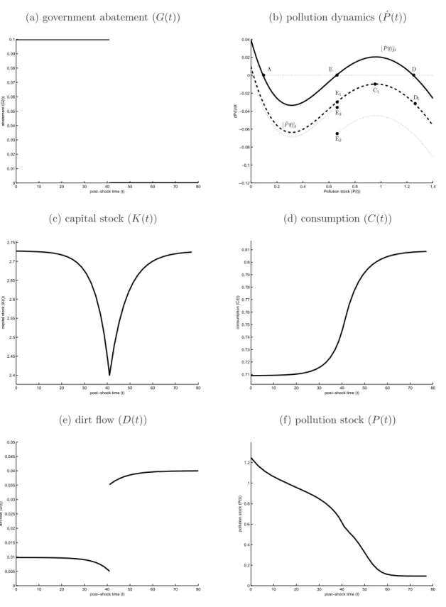
In Figure 3 we visualize the adjustment paths for the key variables using a plausibly calibrated version of the model.

¹⁵

The parameters and key features of the economic and ecological steady states are reported in Table 2. Since ˆ D

₀

is in between the lower and upper threshold values, there exist two stable ecological equilibria – see points A (with ˆ P

G

= 0.0936) and D (with ˆ P

B

= 1.2482) in Figure 3(b). The critical pollution stock associated with ˆ P

₀

is at point E where P

E

= 0.6581.

The shock consists of a temporary increase in government abatement equal to ten percent of initial output, i.e. G = 0.1 for 0 ≤ t < t

E

. The minimum duration for a shock of this size to succeed in steering the ecology to the clean ecological equilibrium is t

E

= 41 years – see Figure 3(a). The other panels in Figure 3 confirm the qualitative results relating to the economy. Panel (c) shows that the capital stock is reduced quite substantially during transition, reaching a minimum of K (t

_E

) = 2.3998. Similarly, as panel (d) shows, private consumption is reduced at impact to C (0) = 0.7092.

The ecological effects are as follows. At impact the abatement shock shifts the ˙ P (t) curve down (from [ ˙ P (t)]

₀

to [ ˙ P (t)]

₁

in panel (b)). For P (t) = ˆ P

B

, the abatement shock ensures

15The parameters of the economic system take the values typically assumed in the macroeconomic literature.

The resulting steady-state interest rate, capital-output ratio, and output shares of consumption and investment are quite realistic. Much less is known about the parameters of ecological system. We have chosen these parameters such that the initial steady-state is in the region with multiple equilibria.

Figure 3: Dynamic effects of government abatement: Core model

(a) government abatement (G(t)) (b) pollution dynamics ( ˙P(t))

0 10 20 30 40 50 60 70 80

0 0.01 0.02 0.03 0.04 0.05 0.06 0.07 0.08 0.09 0.1

post−shock time (t)

abatement (G(t))

0 0.2 0.4 0.6 0.8 1 1.2 1.4

−0.12

−0.1

−0.08

−0.06

−0.04

−0.02 0 0.02 0.04

Pollution stock (P(t))

dP(t)/dt

•A ^E•

E1

•

E3

•

E2

•

C1

•

D•

D1

[ ˙P(t)]0

[ ˙P(t)]1

•

(c) capital stock (K(t)) (d) consumption (C(t))

0 10 20 30 40 50 60 70 80

2.4 2.45 2.5 2.55 2.6 2.65 2.7 2.75

post−shock time (t)

capital stock (K(t))

0 10 20 30 40 50 60 70 80

0.71 0.72 0.73 0.74 0.75 0.76 0.77 0.78 0.79 0.8 0.81

post−shock time (t)

consumption (C(t))

(e) dirt flow (D(t)) (f) pollution stock (P(t))

0 10 20 30 40 50 60 70 80

0 0.005 0.01 0.015 0.02 0.025 0.03 0.035 0.04 0.045 0.05

post−shock time (t)

dirt flow (D(t))

0 10 20 30 40 50 60 70 80

0 0.2 0.4 0.6 0.8 1 1.2

post−shock time (t)

pollution stock (P(t))

Parameters: see Table 2. The initial ecological equilibrium is at point D in panel (b).

that the stock of pollution starts to fall at impact, i.e. at point D

₁

in panel (b) ˙ P (0) < 0.

Two things happen over time. First, the pollution stock gradually declines as ˙ P (t) < 0, for t ≥ 0. Second, the dashed ˙ P (t) line itself gradually shifts down in the direction of the thin dotted line as a result of capital crowding out. At time t

E

= 41, the ecology arrives at point E

₂

in panel (b), shortly thereafter P (t) < P

_E

, the abatement policy is terminated, and the P ˙ (t) line immediately shifts up to the thin dotted directly line below [ ˙ P (t)]

₀

. The ecology jumps from E

₂

to E

₃

in panel (b). Thereafter, the gradual increase in the capital stock shifts the ˙ P (t) line back to [ ˙ P (t)]

₀

and the ecology converges to point A. Panels (e) and (f) of Figure 3 depict the time paths of, respectively, the flow of dirt and the pollution stock. The new ecological equilibrium is attained after more than sixty years.

Points D and A feature the same steady-state value for consumption but environmental quality is much higher in the latter point, so it follows that steady-state welfare is higher after the abatement policy. But is welfare also increased when we take the transitional dynamic effects on consumption and the pollution stock into account? Since the shock occurs at time t = 0, welfare is given by:

Λ

A

(0) ≡ Z

∞

0

h ln C(t) + ε

E

ln E ¯ − P (t) i

· e

^−ρt

dt. (13)

Using the values for ε

E

and ¯ E from Table 2, as well as the solution paths for C (t) and P (t) during transition, we find that Λ

A

(0) = −5.890 with the abatement policy. At the initial dirty equilibrium, welfare is:

Λ

D

(0) = 1 ρ ·

h

ln ˆ C + ε

E

ln[ ¯ E − P ˆ

B

] i

, (14)

which is equal to Λ

D

(0) = −11.71. The welfare gain in utility terms is thus equal to

∆Λ (0) ≡ Λ

_A

(0) − Λ

_D

(0) = 5.82. To facilitate the interpretation of this gain we compute an “equivalent-variation” type welfare measure by computing what ˆ C would have to be in (14) to get ∆Λ (0) to be zero. Denoting this hypothetical consumption level by ˆ C

^′

we find C ˆ

^′

= e

^{ρΛA(0)−εEln}

[

^{E−¯ Pˆ}B

]. An interpretable welfare measure is then:

EV (0) ≡ 100 · C ˆ

^′

− C ˆ

C ˆ . (15)

Intuitively, EV (0) represents consumption that is missed out on if the abatement policy is

not pursued. For the policy combination (G, t

E

) = (0.1, 41) we find that EV (0) is 26.3%, i.e.

lost consumption is more than one quarter of actual consumption at point D and the welfare gains of abatement are huge.

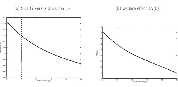
As was mentioned above, there is a trade-off between the size of the abatement shock (G) and its duration (t

E

). We provide quantitative evidence for this trade-off in Figure 4(a).

This figure plots the minimum shock size for shock durations ranging from 25 to 50 years.

¹⁶

For t

E

= 41 a value of G = 0.1 is sufficient, but for t

E

= 30 the shock must be increased to G = 0.1166, whilst for t

_E

= 25 it must be set at G = 0.1293. In short, Figure 4(a) shows that the size-duration locus is downward sloping. Not all points along the size-duration locus are feasible. Indeed, points to the left of the vertical dashed line are infeasible because the dirt flow constraint, D (t) ≥ 0, is violated for some t during transition. It follows that only the size-duration locus to the right of the dashed line is feasible.

The clear trade-off between shock size and duration takes us to the social welfare issue.

What is better from a welfare-theoretic point of view, a long-lasting small shock, or a short- lasting big shock? Figure 4(b) plots the optimized values of Λ (0) for different values of t

E

(and the associated values of G implied by the trade-off). It is clear from the figure that a

“cold turkey” abatement policy is optimal, i.e. to get from D to A in Figure 1, the duration should be as small as possible and the shock size as large as needed. Indeed, for the cold turkey combination (G, t

E

) = (0.1166, 30) we find that EV (0) is a whopping 33.7% of initial consumption.

Of course, there is another welfare question that can be posed. Given that the ecology is located in the dirty equilibrium at point D in Figure 1, where on the lower branch of the P ˙ (t) = 0 curve should the new equilibrium be moved to? As we show in Appendix A, the first-best social optimum calls for a non-zero tax on capital (θ

K

> 0) and no abatement (G = 0) in the long run. This establishes a new ecological equilibrium to the left of point A as the Pigouvian capital tax internalizes the polluting effects of the capital stock. The first-best equilibrium values are ˆ K

f

= 2.3177, ˆ Y

f

= 0.9524, ˆ C

f

= 0.7901, and ˆ P

f

= 0.0766, whilst the Pigouvian capital tax equals θ

K

= 0.1077.

In the absence of capital taxation, however, the first-best social optimum cannot be decen- tralized as privately optimal savings behaviour leads to the equalization of the net marginal product of capital and the rate of time preference, so that the capital stock is equal to ˆ K

16FortE<25 there is no feasible solution for the shock size.

Figure 4: Size, duration, and welfare

(a) SizeGversus durationt_E (b) welfare effect (Λ(0))

25 30 35 40 45 50

0.08 0.085 0.09 0.095 0.1 0.105 0.11 0.115 0.12 0.125 0.13

Shock duration (t E)

Shock size (G)

25 30 35 40 45 50

−7.5

−7

−6.5

−6

−5.5

−5

−4.5

−4

−3.5

−3

Shock duration (t E)

Welfare

(> K ˆ

_f

). As we show in Appendix B, however, the second-best social optimum still calls for zero abatement in the long run. Since the second-best steady-state capital stock equals K ˆ

_s

= ˆ K, it follows that ˆ Y

_s

= ˆ Y , ˆ C

_s

= ˆ C, ˆ D

_s

= ˆ D

₀

, and ˆ P

_s

= ˆ P

_G

. Lacking a Pigouvian tax instrument, it is optimal for the policy maker to engineer the move from D to A in the fastest way possible. Figure 4(a)–(b) illustrate this point.

4 Extensions

In this section we study two extensions to the core model. The first extension endogenizes the labour supply decision of the infinitely lived representative agent. In such a setting, a tax- financed abatement policy expands labour supply (as people get poorer), the capital stock, and output. This dirties the environment and makes it harder to steer the ecology from the dirty to the clean steady-state equilibrium.

In the second extension we take labour supply to be exogenous (as in the core model) but assume that the economy is populated by overlapping generations of finitely-lived agents.

As in the core model, a tax-financed abatement policy crowds out the capital stock during

transition. Unlike the core model, however, the overlapping generations model features in-

tergenerational redistribution (both during transition and in the long run). This opens up

a useful role for public debt policy, namely to redistribute uneven welfare effects. The debt policy itself introduces hysteresis into the economic system in that a deficit-financed tempo- rary abatement policy causes a permanent effect on the capital stock, consumption, output, wages , and the interest rate.

4.1 Endogenous labour supply

In the first extension we change the utility functional of the representative agent from (3) to:

Λ(t) ≡ Z

∞

t

ln h

C(τ )

^εC

· [1 − L(τ )]

^1−εC

i

+ ε

E

ln E ¯ − P (τ )

· e

^ρ(t−τ)

dτ , (16) with 0 < ε

C

< 1. Here, L(τ ) is labour supply and, since the time endowment is equal to unity, 1 − L(τ ) represents the amount of leisure consumed by the household. The household’s budget identity (4) is changed to reflect the endogeneity of labour supply:

A ˙ (τ ) = r(τ )A(τ ) + w(τ )L (τ ) − T (τ ) − C(τ ), (17) where w(τ )L (τ ) represents labour income in period τ .

The representative agent chooses time profiles for C(τ ), L (τ ), and A (τ ) which maximize (16) subject to (17) and a solvency requirement. The solutions for consumption and labour supply in the planning period t amounts are:

C(t) = ρε

C

· [A(t) + H(t)], w (t) · [1 − L (t)] = ρ (1 − ε

C

) · [A(t) + H(t)], (18) where H (t) is defined in (6) above. Optimal consumption growth is still as given in (7) above.

By combining the two expressions in (18), we find that the optimal labour supply decision leads to an equalization of the marginal rate of substitution between leisure and consumption to the wage rate, or:

L (t) = 1 − 1 − ε

C

ε

C

· C (t)

w (t) . (19)

Equation (19) replaces (T1.6) in Table 1.

The phase diagram for the endogenous labour supply (ELS) model is given in Figure 5. In contrast to the core model, the ELS model features a downward sloping ˙ C (t) = 0 line.

¹⁷

For

17For all point on the ˙C(t) = 0 line, ρ+δ =FK(K/L,1), i.e. there is a constant labour-capital ratio, ˆl≡L/K. Labour market equilibrium then implies that the ˙C(t) = 0 line can be written as:

C(t) = εCεL

1−εC

ˆl^εL−1·

h1−ˆl·K(t)i .

C(t)

K(t)

!

! 0

!

! E

0

E

₁

C(0)

(K(t) = 0) .

₀

(K(t) = 0) .

₁

C(t) = 0 .

C ˆ

K ˆ

B

!

SP

₀

A C

!

Figure 5: Consumption-capital dynamics with endogenous labour supply

points above (below) the ˙ C (t) = 0 line, consumption is too high (low), labour supply is too low (high), the capital-labour ratio is too high (low), the interest rate falls short of (exceeds) the rate of time preference, and consumption falls (rises) over time. The dynamics for the capital stock is qualitatively the same as in the core model, and the ELS model features a unique steady state at point E

₀

.

A temporary abatement policy of the form given in (12) gives rise to the adjustment path in Figure 5, consisting of an immediate jump from E

₀

to point A, a gradual move from A to B and C, and a gradual move from C back to point E

₀

. The intuition is as follows. At impact the tax increase reduces human wealth, H (0), which prompts the agent to cut the consumption of goods and leisure, i.e. labour supply increases. Provided the policy is of sufficiently long duration, point A lies below the [ ˙ K (t) = 0]

₁

line and the agent saves part of the additional wage income. Since the capital-labour ratio is low, the interest rate is high and both consumption and the capital stock increase over time immediately after the shock.

This explains the gradual move from A to B.

At some time 0 < t < t

E

the economy arrives at point B, after which capital decumulation

takes place but consumption continues to grow. At time t = t

E

, the economy is at point C, the

abatement policy is terminated, and the capital equilibrium locus shifts back to [ ˙ K (t) = 0]

₀

. From then on the dynamic forces are such as to increase both consumption and capital as the economy moves from C to E

₀

.

An interesting feature of the transition path for the capital stock is its non-monotonicity.

More importantly, at least during the early transition phase capital is crowded in as a result of the tax-financed abatement shock, a phenomenon which complicates environmental policy because it leads to an increase in the flow of dirt. So whereas capital decumulation helps environmental policy in the core model during the early phases, it hinders policy in the ELS model.

To investigate the quantitative significance of the negative feedback effect via the capital stock we calibrate and simulate the ELS model. For ρ, δ, ε

_L

, κ, and γ we use the same parameters as before – see Table 2. We choose ε

C

such that the steady-state intertemporal labour supply elasticity, (1 − L)/ ˆ L, is equal to two. This gives ˆ ε

_C

= 0.3663 and ˆ L = 1/3.

Finally, we choose Ω

₀

such that steady-state output is equal to unity, ˆ Y = 1. This gives Ω

₀

= 1.5969.

Figure 6 illustrates the transition paths for a shock featuring G = 0.1. The minimum feasible duration for this shock is t

E

= 52 years! Despite the fact that the core model and the ELS model are initially in an identical steady state (as far as output, consumption, the capital stock, and pollution are concerned), the abatement policy must be maintained for a much longer period than in the core model when labour supply effects are taken into account. In a quantitative sense, therefore, the capital-feedback effect is significant. As is shown in panel (b), the capital stock features large fluctuations, reaching a maximum of about 2.95 for much of the early transition phase, and a minimum of K (t

E

) = 2.6106. Similarly, output reaches a maximum of about 1.08 reflecting the large spending multiplier that exists in the ELS model (see also Heijdra, 2009, p. 511). Using the welfare measure developed above in (15), we find that for the policy combination (G, t

E

) = (0.1, 52), EV (0) is 7.8%. Recall that in the core model there was a welfare gain of 26.3% for the policy combination (G, t

E

) = (0.1, 41), so the labour supply effect reduces the welfare gains of moving from the dirty to the clean equilibrium.

Just as in the core model, there is no welfare-enhancing role for long-run abatement in

the ELS model. A permanent abatement policy would shift the economic equilibrium from

(a) capital stock (K(t)) (b) consumption (C(t))

0 10 20 30 40 50 60 70 80 90 100

2.6 2.65 2.7 2.75 2.8 2.85 2.9 2.95

post−shock time (t)

capital stock (K(t))

0 10 20 30 40 50 60 70 80 90 100

0.74 0.75 0.76 0.77 0.78 0.79 0.8 0.81

post−shock time (t)

consumption (C(t))

(c) output (Y(t)) (d) employment (L(t))

0 10 20 30 40 50 60 70 80 90 100

0.99 1 1.01 1.02 1.03 1.04 1.05 1.06 1.07 1.08 1.09

post−shock time (t)

output (Y(t))

0 10 20 30 40 50 60 70 80 90 100

0.335 0.34 0.345 0.35 0.355 0.36 0.365 0.37

post−shock time (t)

employment (L(t))

(e) dirt flow (D(t)) (f) pollution stock (P(t))

0 10 20 30 40 50 60 70 80 90 100

0 0.005 0.01 0.015 0.02 0.025 0.03 0.035 0.04 0.045 0.05

post−shock time (t)

dirt flow (D(t))

0 10 20 30 40 50 60 70 80 90 100

0 0.2 0.4 0.6 0.8 1 1.2

post−shock time (t)

pollution stock (P(t))

Figure 6: Dynamic effects of government abatement: Endogenous labour supply

E

₀

to E

₁

in Figure 5, and would result in a permanently higher steady-state capital stock and thus a higher dirt flow. The economy would move further away from the first-best optimum.

In short, both the first-best and the second-best social optimum call for the smallest feasible abatement level in the long run, i.e. for G = 0.

4.2 Finite lives

In the second extension we take labour supply to be exogenous but assume that individuals face an age-independent probability of death, µ. In particular, we use the Blanchard (1985) model of consumer behaviour. At time t, expected remaining lifetime utility of an individual born at time v (v ≤ t) is given by:

E Λ (v, t) ≡ Z

∞

t

h

ln C(v, τ ) + ε

E

ln E ¯ − P (τ ) i

· e

^{(ρ+µ)(t−τ)}

dτ , (20)

where C (v, τ) is consumption, ρ is the pure rate of time preference, and µ is the instantaneous mortality rate. With a positive mortality rate, future felicity is discounted more heavily than in the representative-agent model because the mortal agent simply may not be alive to enjoy felicity in the future – see Yaari (1965). Following Blanchard (1985) and Yaari (1965), we assume that there exist perfect annuities. The actuarially fair annuity rate of interest is equal to r (τ ) + µ and rational individuals fully annuitize because it expands their choice set. The agent’s budget identity is thus given by:

A(v, τ ˙ ) = [r (τ ) + µ] A(v, τ) + w(τ ) − C(v, τ ) − T (τ ) , (21) where A (v, τ ) is the stock of financial assets at time τ of an agent born at time v. Newborn agents are born without financial assets, i.e. A (v, v) = 0.

An agent born of vintage v chooses time profiles for C(v, τ ) and A (v, τ ) which maximize (20) subject to (21) and a solvency requirement. The solution for consumption in the planning period t amounts to:

C(v, t) = (ρ + µ) · [A(v, t) + H(t)], (22)

where expected life-time human wealth at that time, H(t), is given by:

H(t) ≡ Z

∞

t

[w(τ ) − T (τ )] · e

^{−Rtτ[r(s)+µ]ds}

dτ . (23)

The optimal time profile for individual consumption is of the same form as (7):

C ˙ (v, τ )

C (v, τ ) = r (τ ) − ρ, τ ≥ t ≥ v. (24)

In (22) the mortality rate features in the propensity to consume out of total wealth because mortality is yet another reason to be impatient. In (23) the mortality rate features because agents use the annuity rate of interest to discount after-tax non-asset income. Importantly, the annuity rate drops out of the individual consumption growth equation because annuities are perfect; a result first demonstrated by Yaari (1965, p. 147).

We assume that the crude birth rate is equal to the mortality rate so that (i) the aggregate population is constant and can be normalized to unity, and (ii) the relative population size of cohort v at time t (> v) is given by µe

^−µ(t−v)

. Aggregate variables can thus be calculated as the weighted sum of the values for different generations, e.g. C(t) ≡ R

t

−∞

C(v, t)µe

^−µ(t−v)

dv is aggregate consumption. By aggregating (24), we arrive at the aggregate consumption growth equation:

C(t) ˙

C(t) = r (t) − ρ − µ(ρ + µ) · A(t)

C(t) = C(v, t) ˙

C(v, t) − µ · C(t) − C(t, t)

C(t) . (25)

Equation (25) has the same form as the Euler equation for individual households (24), except for a correction term capturing the wealth redistribution caused by the turnover of genera- tions. Optimal individual consumption growth is the same for all generations since they face the same rate of interest. But the consumption level of old generations is higher than that of young generations, reflecting the larger stock of financial assets owned by old generations. Be- cause existing generations are continually being replaced by newborns, who are born without financial wealth, aggregate consumption growth falls short of individual consumption growth.

The correction term appearing in (25) thus represents the difference in average consumption, C(t), and consumption by newborns, C(t, t).

A well-known property of the Blanchard-Yaari model concerns the non-neutrality of public debt. In the presence of public debt, the capital market equilibrium condition is given by A (t) = K (t) + B (t) so that consumption growth equation is given by:

C(t) ˙

C(t) = r (t) − ρ − µ(ρ + µ) · K (t) + B(t)

C(t) . (26)

Equation (26) replaces replaces (T1.1) in Table 1.

K(t) E

₀

K ˆ

^RA

C(t)

(K(t) = 0)

0

.

C(t) = 0 .

A

!

! E

₁

(K(t) = 0) .

₁

B

C

!

! ! C ˆ

K ˆ

SP

0

Figure 7: Consumption-capital dynamics with overlapping generations

The phase diagram for the overlapping generations (OG) model is given in Figure 7. We assume that public debt is equal to zero initially. In contrast to the core model, the OG model features an upward sloping ˙ C (t) = 0 line.

¹⁸

For points above (below) the ˙ C (t) = 0 line, the generational turnover term is relatively small (large), the interest rate exceeds (falls short of) the rate of time preference, and consumption rises (falls) over time. The dynamics for the capital stock is exactly the same as in the core model, and the OG model features a unique steady state at point E

0

.

A temporary abatement policy of the form given in (12) gives rise to the adjustment path E

0

ABCE

0

in Figure 5. The intuition is as follows. The shock shifts the capital equilibrium locus to [ ˙ K (t) = 0]

₁

. At impact the tax increase reduces human wealth for all agents, H (v, 0), which prompts them reduce consumption. This is the jump from E

₀

to A directly below it.

At point A the interest rate is unchanged, but the generational turnover term is increased so aggregate consumption gradually falls. Aggregate consumption, however, is too high to

18The ˙C(t) = 0 line is given by:

C(t) = µ(ρ+µ)K(t) FK(K(t),1)−(ρ+δ).

It is horizontal for K(t) = 0 and becomes vertical forK(t)→Kˆ^RA, where ˆK^RA is the steady-state capital stock in the core model (i.e. ρ+δ=FK( ˆK^RA,1).

maintain the initial capital stock ˆ K so capital starts to decumulate. At some time 0 < t < t

_E

the economy arrives at point B, after which aggregate consumption starts to increase even though the capital stock continues to fall. At time t = t

_E

, the economy is at point C, the abatement policy is terminated, and the capital equilibrium locus shifts back to [ ˙ K (t) = 0]

₀

. From then on the dynamic forces are such as to increase both consumption and capital as the economy moves from C to E

₀

.

The transition paths for the core model and the OG model are qualitatively very similar.

The abatement shock cause temporary crowding out of capital, a feature which aids the environmental cleanup. To glean the quantitative significance of this effect we once again calibrate and simulate the model. This time we use the same parameters for δ, ε

L

, Ω

₀

, κ, and γ as in the core model – see Table 2. We assume that the birth/mortality rate is µ = 0.015 and choose ρ such that the initial steady-state interest rate is the same as in the core model (ˆ r = 0.04). This gives ρ = 0.0374. The initial steady state is “observationally equivalent” to the steady state for the core model, i.e. ˆ Y = 1, ˆ K = 2.7273, ˆ I = 0.1909, and ˆ C = 0.8091.

At these parameter values, a shock of G = 0.1 succeeds in moving the ecology to the clean equilibrium provided t

E

= 38 years. Hence, in the OG model the capital stock effect exerts a stronger effect on the environmental cleanup than in the core model.

The distribution of costs and benefits of environmental policy is very uneven in the OG model. In the scenario discussed so far, the costs are borne by all pre-shock generations (whose v < 0) and all post-shock generations born before the policy is terminated (for whom 0 ≤ v < t

E

). Generations born after t

E

do not have to pay any taxes but benefit fully from the environmental cleanup, more so the later they are born. Generalizing the welfare measure given in (15) to the BY model (see Appendix C), we find for shock-time newborns EV (0, 0) = 10.8% and for steady-state newborns EV (∞, ∞) = 33.5%.

The uneven distribution of costs and benefits can be repaired by the policy maker because public debt is non-neutral in the OG model. Both the economic allocation and the inter- generational welfare implications of the abatement policy depend on the way the government balances its budget. The periodic budget identity can be written as follows:

B ˙ (τ ) = r(τ )B(τ ) + G(τ ) − T (τ ). (27)

The government can finance its spending by either issuing more debt ( ˙ B(τ ) ≡ dB(τ )/dτ >

0) or by levying lump-sum taxes (T (τ )). The No Ponzi Game condition ensures that the