Stochastic inference from snapshots of the non-equilibrium steady state: the asymmetric Ising model and beyond

pr obabilities

configurations stationary?

propagate with model

relative entropy Data

pr obabilities

configurations

Stochastic inference from snapshots of the non-equilibrium steady state:

the asymmetric Ising model and beyond

Dissertation Simon Lee Dettmer

Köln 2017

of the non-equilibrium steady state:

the asymmetric Ising model and beyond

Inaugural-Dissertation zur

Erlangung des Doktorgrades

der Mathematisch-Naturwissenschaftlichen Fakult¨at der Universit¨at zu K¨oln

vorgelegt von

Simon Lee Dettmer

aus Oberhausen

K¨oln, 2017

Tag der m¨undlichen Pr¨ufung: 05. Oktober 2017

In dieser Arbeit untersuchen wir das Problem der Parameter-Inferenz f¨ur ergodische Markov-Prozesse, die gegen einen station¨aren Zustand konvergieren, der nicht durch die Boltzmann-Verteilung beschrieben wird. Unser Hauptergebnis ist, dass wir die Pa- rameter verschiedener Modelle auf der Grundlage von unabh¨angigen Stichproben aus dem station¨aren Zustand lernen k¨onnen, obwohl wir die station¨are Wahrscheinlichkeits- verteilung nicht kennen. Genauer: f¨ur die untersuchten Modelle in stetiger Zeit konnten wir die Parameter bis auf einen Skalierungsfaktor inferieren, welcher die Zeitskala bes- timmt, die nat¨urlich nicht aus statischen Messungen ermittelt werden kann; bei Mod- ellen in diskreter Zeit ist die Zeitskala bereits implizit durch die Diskretisierung gew¨ahlt und wir konnten alle Parameter der untersuchten Modelle inferieren. Als Paradigma f¨ur Nicht-Gleichgewichts-Prozesse untersuchen wir das asymmetrische Ising-Modell mit Glauber-Dynamik. Es beschreibt bin¨are Spinvariablen mit asymmetrischen paar- weisen Wechselwirkungen unter dem Ein fl uss ¨außerer Magnetfelder. Diese Magnet- felder und Wechselwirkungsst¨arken wollen wir lernen. Zu diesem Zweck haben wir in dieser Arbeit zwei verschiedene Inferenzmethoden entwickelt: die erste Methode basiert auf der Berechnung von Magnetisierungen, sowie Zwei- und Dreipunkt-Spin- Korrelationen, zum einen in einer selbstkonsistenten Form, die exakt ist, und zum an- deren in einer geschlossenen Form innerhalb einer Molekularfeld-N¨aherung; die zweite Methode beruht auf der Maximierung einer Funktion, die wir ”propagator likelihood”

nennen. Diese betrachtet fi ktive ¨ Uberg¨ange zwischen allen gemessenen Kon fi guratio-

nen und ist verwandt mit der bekannten Log-Likelihood-Funktion f¨ur Gleichgewichts-

Systeme. Der Vorteil des Molekularfeld-Ansatzes ist sein vergleichbar geringer nu-

merischer Aufwand, w¨ahrend der Vorteil des ”propagator likelihood”-Verfahrens darin

besteht, dass es die gesamte empirische Verteilung verwendet und leicht auf jeden er-

godischen Markov-Prozess angewandt werden kann. Insbesondere wenden wir die ”prop-

agator likelihood”-Methode auf weitere bekannte Nicht-Gleichgewichtsmodelle aus der

Statistischen Physik und der Theoretischen Biologie an: den einfachen asymmetrischen

Exklusionsprozess (ASEP) in stetiger Zeit mit diskreten Kon fi gurationen, sowie die

Replikatordynamik in stetiger Zeit mit kontinuierlichen Kon fi gurationen. Die Allge-

meing¨ultigkeit des ”propagator likelihood”-Ansatzes wird dadurch betont, dass er di-

rekt aus dem Prinzip hergeleitet werden kann, dass die gemessene Verteilung station¨ar

unter der Dynamik sein soll, das heißt wir minimieren die relative Entropie zwischen

der empirischen Verteilung und einer Verteilung, die durch eine Zeitentwicklung dieser

empirischen Verteilung erzeugt wird. Schließlich untersuchen wir noch eine etwas an-

dere Situation und zeigen wie die Inferenz im asymmetrischen Ising-Modell verbessert

werden kann, wenn wir mehrere Datens¨atze aus unabh¨angigen Stichproben von ver-

schiedenen station¨aren Zust¨anden haben, die durch kontrollierte St¨orungen der zugrunde

liegenden Modellparameter erzeugt werden.

In this thesis we study the problem of inferring the parameters of ergodic Markov pro-

cesses that converge to a non-equilibrium steady state. Our main result is that for many

models, we can learn the parameters based on independent samples taken from the

steady state, even though we do not know the stationary probability distribution. To

be more precise: for the investigated models in continuous time, we could infer the pa-

rameters up to a factor that defines the time scale, which, naturally, cannot be determined

from static measurements; for the investigated models in discrete time, the time scale

is already chosen implicitly by the discretisation and we could infer all parameters. As

our main paradigm for non-equilibrium inference problems, we study the asymmetric

Ising model with Glauber dynamics. It consists of binary spins subject to external fi elds

and asymmetric pairwise spin-couplings, which we seek to infer. For this purpose we

have developed two different inference methods: the fi rst method is based on computing

magnetisations, two- and three-point spin correlations, either in a self-consistent form

that is exact, or in a closed form within a mean fi eld approximation; the second method

is based on maximising a “propagator likelihood”, which considers fi ctitious transitions

between all sampled con fi gurations and is akin to the well-known log-likelihood func-

tion used for equilibrium systems. The advantage of the mean fi eld approach is its

computational ef fi ciency, while the advantage of the propagator likelihood method is

that it uses information from the full sampled distribution and can easily be applied to

any ergodic Markov process. In particular, we apply the propagator likelihood method

to other prominent non-equilibrium models from statistical physics and theoretical bi-

ology: (i) the asymmetric simple exclusion process (ASEP) in continuous time with

discrete con fi gurations and (ii) replicator dynamics in continuous time with continuous

con fi gurations. The generality of this approach is emphasised by the fact that we can

derive the propagator likelihood directly from the principle that the sampled distribution

should be stationary under the model dynamics: we minimise the relative entropy be-

tween the sampled distribution and a distribution generated by propagating the sampled

distribution in time. Finally, we investigate a slightly different setting: we show how in-

ference can be improved in the asymmetric Ising model by considering multiple sets of

independent samples taken from several steady states, which are generated by controlled

perturbations of the underlying model parameters.

I would like to acknowledge Chau Nguyen, not only for his collaboration and

thoughtful comments concerning the project on mean fi eld inference, but also for

the enjoyable experience of teaching statistical physics classes together, where in

numerous discussions he was so kind to share with me his thorough understand-

ing of the subject. Further, I owe many thanks to my supervisor, Johannes Berg,

not only for presenting me with the problem of non-equilibrium inference, but

also for his continuous support, time, and faith, all of which he gave generously.

1 Introduction 1

1.1 Thesis overview . . . . 1

1.2 Markov processes . . . . 2

1.2.1 Discrete con fi gurations: Markov chains . . . . 4

1.2.2 Continuous con fi gurations . . . . 9

1.2.3 Equilibrium versus non-equilibrium steady states . . . . 19

1.3 Stochastic inference . . . . 25

1.3.1 The Bayesian framework and maximum likelihood . . . 27

1.3.2 Equilibrium inference from snapshots of the steady state 31 1.3.3 Non-equilibrium inference from time-series data . . . . 35

2 The asymmetric Ising model 37 2.1 The model and its history . . . . 37

2.2 Glauber dynamics . . . . 38

2.2.1 Interaction symmetry and detailed balance . . . . 40

2.2.2 Callen’s identities . . . . 42

2.3 Connection with neural networks . . . . 44

2.4 Stochastic inference from time-series data . . . . 46

2.4.1 Maximum likelihood of time-series . . . . 46

2.4.2 The Gaussian mean fi eld theory and time-shifted corre- lations . . . . 50

3 Self-consistent equations and non-equilibrium mean fi eld theory 55 3.1 The general theory . . . . 56

3.1.1 Deriving self-consistent equations . . . . 56

3.1.2 Exact inference based on direct sample averages of the self-consistent equations . . . . 59

3.1.3 Expanding the self-consistent equations with non-equilibrium mean fi eld theory . . . . 60

3.2 Inference in the asymmetric Ising model . . . . 66

3.2.1 Callen’s identities and their mean fi eld expansion . . . . 66

3.2.2 Parameter inference for sequential Glauber dynamics . . 78

3.2.3 Model selection . . . . 79

4 The propagator likelihood 85 4.1 The concept . . . . 85

4.1.1 Minimising relative entropy . . . . 86

4.2 Stochastic inference . . . . 88

4.2.1 Models with discrete con fi gurations (Markov chains) . . 88 4.2.2 Models with continuous con fi gurations . . . . 92 4.2.3 Non-equilibrium models in statistical physics and theo-

retical biology . . . . 95 5 Learning from perturbations in the asymmetric Ising model 105 5.1 General setting and considerations . . . 105 5.2 Mean fi eld inference . . . 106 5.3 Inference with the Gaussian mean fi eld theory . . . 108 5.3.1 Self-consistent equations for the two-point correlations. . 109 5.3.2 Inference from perturbations in sequential Glauber dy-

namics . . . 110

6 Conclusions and Outlook 115

References 121

A Further mean fi eld equations for the asymmetric Ising model 127

A.1 Magnetisations to third order . . . 127

A.2 Correlations under sequential Glauber dynamics . . . 127

A.3 Correlations under parallel Glauber dynamics . . . 129

B Description of the moment-matching inference algorithm 131

1

Introduction

To begin at the beginning

Dylan Thomas

1.1 Thesis overview

This thesis addresses the problem of inferring the parameters of ergodic Markov processes based on independent samples taken from the non-equilibrium steady state.

In this fi rst chapter, we recall the standard results on ergodic Markov pro- cesses concerning the convergence to steady states and their classi fi cation into equilibrium and non-equilibrium steady states. We then formulate our stochastic inference problem and give a brief overview of established inference methods for equilibrium steady states and for time-series data. First, we motivate the max- imum likelihood method within the framework of Bayesian reasoning, before brie fl y mentioning the equilibrium mean fi eld approximation and the pseudo- likelihood method. Second, we discuss inference based on maximum likelihood for time series.

In chapter 2, we give some background on our main paradigm for non- equilibrium inference problems: the asymmetric Ising model. We will introduce Glauber dynamics and show that this dynamics converges to a non-equilibrium steady state for the case of asymmetric couplings between spins; we motivate the consideration of asymmetric couplings by brie fl y discussing the connection of the asymmetric Ising model with neural networks. In the following, we describe Callen’s identities characterising the spin moments, since they will be used for inference in chapters 3 and 5. We discuss maximum likelihood inference based on time-series data and present some minor results we found for inference in sequential Glauber dynamics, before presenting the Gaussian mean fi eld theory of M´ezard and Sakellariou (2011), which we will use for inference in chapter 5.

In chapter 3, we develop our fi rst method for stochastic inference from snap- shots of the steady state, which is based on fi tting sampled observables to self- consistent equations, which we derive as generalisations of Callen’s identities.

We show how these self-consistent equations can be used to infer model param-

eters by replacing steady state expectation values with sample averages. In the

following, we discuss how to approximately evaluate the self-consistent equa-

tions in a closed-form within an expansion around non-equilibrium mean fi eld

theory. The presentation of this expansion was inspired by the work of Kappen

and Spanjers (2000), who developed the non-equilibrium mean fi eld theory for the asymmetric Ising model. Here, we provide a straightforward generalisation of their theory and formulate it for a wider class of ergodic Markov processes.

Finally, we use these methods to address the stochastic inference problem for the asymmetric Ising model.

In chapter 4, we develop our second inference method, based on maximis- ing a function we call the propagator likelihood. We give a derivation of this function based on minimising relative entropy and illustrate the method for sev- eral toy models spanning the different classes of Markov processes, including the Ornstein-Uhlenbeck process and the asymmetric simple exclusion process (ASEP). Then we use the method to infer the parameters of more challenging models: the asymmetric Ising model (again) and replicator dynamics.

In chapter 5, we consider a slightly different setting and investigate how in- ference in the asymmetric Ising model can be improved by considering multiple sets of independent samples, which are taken from several steady states gener- ated by known perturbations of the underlying parameters. We begin with some general considerations concerning the observables required for a well-de fi ned inference problem and discuss the different roles of perturbations of the external fi elds and perturbations of the couplings. Next, we develop a simple inference algorithm based on the expressions for magnetisations and two-point correla- tions obtained in the non-equilibrium mean fi eld theory of chapter 3 and discuss some basic properties of the approach. We follow with a more powerful infer- ence method based on the Gaussian mean fi eld theory of M´ezard and Sakellar- iou (2011), which we use to derive self-consistent equations for the equal-time two-point correlations. In the case of vanishing external fi elds, these equations become linear in the couplings and allow for a computationally highly ef fi cient inference algorithm that can easily be scaled to large system sizes. We investi- gate the performance of this method by considering an example where half of the couplings is set to zero in the perturbation and compare the approach to the setting considered chapters 3 and 4.

Finally, in chapter 6 we summarise and interpret our results in addition to giving a perspective on possible future directions for research. Section 3.2, ap- pendix B, and parts of appendix A were previously published in (Dettmer et al., 2016); chapter 4 has appeared in (Dettmer and Berg, 2017).

1.2 Markov processes

A stochastic process { X ( t )} is a sequence of random variables { X ( t )} t ∈ I , where

the index t denotes time, which could be discrete, I = { 0 , 1 ,..., T } , or continu-

ous, I = [ 0 , T ] , with a possibly in fi nite time horizon T = ∞ . Examples for the ran-

dom variables could be the continuous-time positions of a set of gas molecules, the daily temperature at noon on the roof of Cologne Cathedral, or the weekly draw of lottery numbers. Due to the randomness of the variables we cannot make de fi nite predictions about outcomes, but instead have to content ourselves with statements about the probabilities of different outcomes. This probability may be interpreted as a subjective belief concerning different events occurring (Bayesian interpretation) or as their relative frequencies in the limit of a large ensemble of copies of the process, each taking a different (random) realisation (frequentist interpretation).

Figure 1.1: Andrei Andreye- vich Markov, who researched the stochastic processes nowadays named after him, was less inter- ested in physical applications of these processes but instead pre- ferred to use them for studying poetry.

In general, there will be relationships con- necting the different variables, e.g. given that today the temperature at Cologne Cathedral is 21 ^◦ C, it is highly unlikely that tomorrow the temperature will be − 10 ^◦ C. These relation- ships can be captured by conditional proba- bilities, which tell us how the observed re- alisation of the stochastic process until time t 1 in fl uences the probability of some event A taking place at a later time t ₂ > t ₁ . The inter-dependence of the random variables may be arbitrarily complicated, however, for many applications we can focus on classes of pro- cesses with very simple relationships. The simplest case is when the variables are statisti- cally independent, e.g. knowledge of the past draws of lottery numbers does not in fl uence the probabilities of particular numbers appear- ing in next week’s draw. This case will not be discussed in this thesis. For processes with real inter-dependencies between the variables, the simplest case is when the probability of the future event A depends on the past history of the process only via the present state X ( t 1 ) , i.e.

P ( X ( t ₂ ) ∈ A |{ X ( s )} s ≤ t

) = P ( X ( t ₂ ) ∈ A | X ( t ₁ )) ∀ t ₂ > t ₁ , (1.1)

which is known as the Markov property. Sequences of random variables obey-

ing the Markov property are known as Markov processes, in recognition of

Andrei Markov who studied these processes for the purpose of extending the

weak law of large numbers to random variables that are not statistically inde-

pendent (Markov, 2006; Seneta, 2006). The reason for the widespread use of Markov processes is not just their simplicity, but for many real-world processes it can be argued that the Markov property should hold true with a high degree of accuracy. For example, in the kinetic theory of gases (see e.g. Redner et al.

(2010)) the molecular chaos assumption argues that the trajectories ( x ( t ), v ( t )) of gas particles are effectively Markov processes, due to the great number of particle collisions occurring on time-scales much shorter than the observation time.

Of course not all real-world random processes are Markovian and whether a process obeys the Markov property depends also on the choice of variables.

Consider a point-mass in classical mechanics described by its position x and momentum p. We know that knowledge of the current position x ( t ) is not suf fi - cient to predict the future trajectory of the particle so the position process { x ( t )}

does not obey the Markov property. However, adding the momentum p ( t ) yields the necessary information and the joint process {( x ( t ), p ( t ))} is indeed a Markov process ¹ . In fact, many probabilistic models with memory can be made Markov processes by adding auxiliary variables (see e.g. Lei et al. (2016)).

1.2.1 Discrete con fi gurations: Markov chains

Markov processes can be classi fi ed by (i) whether time is discrete or continu- ous, and (ii) whether the con fi guration space Ω X ( t ) is discrete or continuous.

Markov processes with discrete con fi gurations are called Markov chains. The theory is simplest for these Markov chains and for this reason we pick them as our starting point for an exposition of the standard results on Markov pro- cesses (see e.g. Feller (1968); Gardiner (2009); Grimmett and Stirzaker (2001);

Klenke (2013); Levin and Peres (2008)) most pertinent to the framing our stochas- tic inference problem.

1.2.1.1 Discrete time

We consider a set of n possible con fi gurations Ω = {ω 1 ,..., ω n } , assumed by the random variables X 0 , X 1 , X 2 ,... , where X t is a short-hand for X ( t ) . As exam- ples we can think of the energy levels assumed by a quantum harmonic oscilla- tor, the number of particles present in a subsystem connected to a reservoir of chemical potential µ . The discretisation of time could correspond to measure- ments taking place at fi xed time intervals. In this case, we can use the Markov

1 A free point-mass would of course obey deterministic dynamics, which can be

considered a limiting case of random processes. By adding interactions with a heat

bath we can introduce randomness into the process and the same statement applies.

property to iteratively rewrite the joint probability distribution of a set of ran- dom variables X ₀ , X ₁ ,..., X _k in terms of the single-step conditional probabilities P ( X _t = x _t | X _{t − 1} = x _{t − 1} ) as

P ( X _k = x _k ,..., X ₀ = x ₀ ) = P ( X _k = x _k | X _k−1 = x _k−1 ,..., X ₀ = x ₀ )

× P ( X _k−1 = x _k−1 ,..., X 0 = x 0 )

= P ( X _k = x _k | X _k−1 = x _k−1 ) P ( X _k−1 = x _k−1 ,..., X ₀ = x ₀ )

=... = P ( X ₀ = x ₀ ) _t=1 ∏ ^{k P ( X t = x t | X t − 1 = x t − 1 ) . (1.2)}

The conditional probabilities P ( X _t = x _t | X _{t − 1} = x _{t − 1} ) are also called transition probabilities. The most commonly studied Markov chains are time-homogeneous chains, where the transition probabilities do not depend on the time t of the tran- sition. Hence, the process is fully described by the initial condition P ( X ₀ = x ₀ ) and the matrix of transition probabilities

T _{i j} : = P ( X ₁ = ω j | X ₀ = ω i ) . (1.3) In particular, by summing over intermediate time-steps, the distribution of the random variable at time t, p _i ( t ) : = P ( X _t = ω i ) , can be written as the matrix product of the initial distribution p ( 0 ) and the transition matrix T taken to the power t

p _i ( t ) = [ p ( 0 ) T ^t ] i = ∑ _j=1 ^{n p j ( 0 )( T t ) ji . (1.4)}

For the special case of deterministic initial conditions where the process starts in a con fi guration x ₀ ∈ Ω , i.e. p _j ( 0 ) = δ ω

,x

, we reserve the notation

p ( x , t | x ₀ , 0 ) : = P ( X ( t ) = x | X ( 0 ) = x ₀ ) , (1.5) which is called the propagator, since it takes the probability distribution at time 0 (concentrated in con fi guration x ₀ ) and propagates this distribution forward in time to create the probability distribution at time t. Due to the linearity of the equations, we can write the solution for an arbitrary initial condition p ( 0 ) as a sum over propagators

p _i ( t ) = ∑ _j=1 ^{n p (ω i , t |ω j , 0 ) p j ( 0 ) . (1.6)}

T HE STEADY STATE AND CONVERGENCE OF THE M ARKOV CHAIN

Under certain conditions on the transition matrix T , the single-time distribution

p ( t ) converges to a unique distribution π , called the steady state (or stationary

distribution), independent of the initial probability distribution p ( 0 ) . We call these chains ergodic. It is clear that the steady state has the property of remain- ing unchanged when propagating the distribution with the transition matrix

π = π T , (1.7)

which we use as the de fi nition of a steady state.

In some cases one or more steady states may exist, but the Markov chain might not converge for arbitrary initial conditions. For chains with fi nite con- fi guration space, |Ω| < ∞ , the existence and uniqueness of the steady state is guaranteed by the condition of irreducibility, stating that the chain can reach any con fi guration from any starting point in a fi nite number of steps with pos- itive transition probability. These are the most studied chains and all Markov chains considered in this thesis will be irreducible. Markov chains that are not irreducible can be divided into irreducible sub-chains and then only the transi- tions between the subclasses have to be accounted for additionally. For in fi nite con fi guration spaces, |Ω| = ∞ , irreducibility is not suf fi cient to ensure the ex- istence of a normalisable steady state. In addition, we require that the average time of return to any initial con fi guration is fi nite. These chains are called posi- tive recurrent. The Markov chain actually converges to the unique steady state, independent of the initial condition, if the chain is aperiodic. In an aperiodic chain, the possible paths that start from an initial con fi guration and return to the starting point must not have a common divisor to their number of steps. An ex- ample for a periodic chain is the simple random walk on Z , where the chain hops one place to the left or one place to to right in every time step, so the chain can return to a con fi guration only after an even number of steps.

The results above on the convergence of Markov chains have been known for a long time. More recently, people have studied how long the Markov chain ac- tually takes to converge to the steady state and how this time depends on the size of the con fi guration space; this fi eld is known as Markov mixing times (Levin and Peres, 2008).

E XAMPLE : BIASED RANDOM WALK ON N 0

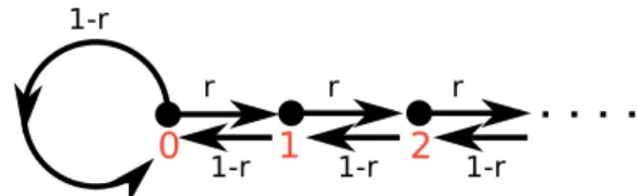
The biased random walk on N 0 is most simply de fi ned by a picture of the chain’s con fi gurations and transition probabilities (Fig. 1.2).

In each time step, the chain moves one place to the right with probability

r, or one place to the left with probability 1 − r, except when the chain is in 0

where instead of moving to − 1, the chain remains in 0. The chain is obviously

irreducible and aperiodic, since the chain can remain in 0 for an arbitrary number

of time steps. The chain therefore converges to a unique steady state if and

only if the chain is positive recurrent. We can check this condition by actually

r

0 _1-r 1 2

1-r

r r

1-r 1-r

Figure 1.2: Schematic view of the transition rules for the biased random walk on N 0 .

computing the steady state. The steady state de fi ning equation (1.7) becomes r π i−1 + ( 1 − r )π i+1 = π i , i = 1 , 2 ,... (1.8) ( 1 − r )π 0 + ( 1 − r )π 1 = π 0 . (1.9) These equations can be solved iteratively and we obtain

π i = r

1 − r _i

π 0 . (1.10)

The steady state is normalisable if and only if r /( 1 − r ) < 1 ⇔ r < 1 / 2:

1 = ∑ ^∞

i = 0

π i = ∑ ^∞

i = 0

r 1 − r

i

π 0

r 1−r

<1

= 1 − r

1 − 2r π 0 . (1.11) Thus, for r < 1 / 2 the chain is positive recurrent and we have a normalisable steady state. It can be shown (Klenke, 2013) that (i) for r > 1 / 2 the chain is transient and wanders off to in fi nity so any con fi guration is visited only fi nitely many times; (ii) for r = 1 / 2 we have a null-recurrent chain, i.e. each con fi gura- tion is visited in fi nitely often, but the mean return time is in fi nite.

1.2.1.2 Continuous time

Markov chains in continuous time have no memory of how long they have re- mained in a certain con fi guration. The transitions are therefore described by in- stantaneous transition rates K i j ( t ) , giving the probability that the chain jumps from con fi guration ω i to con fi guration ω j within the in fi nitesimal time interval [ t , t + dt ) . We can de fi ne them as the limit

K _{i j} ( t ) : = lim

δt→ 0 P ( X ( t + δ t ) = ω j | X ( t ) = ω i )/δ t . (1.12)

As for the discrete-time Markov chains, we focus on time-homogeneous chains

where the transition rates do not depend on time, K _{i j} ( t ) ≡ K _{i j} . The random

time τ that the chain remains in a given con fi guration ω i is then exponentially

distributed with parameter λ i = ∑ j=i K _{i j} > 0 and we can de fi ne a corresponding transition matrix in discrete time as

T _{i j} =

K _{i j} /λ i i = j

0 i = j , (1.13)

where we count time in units of the (random) jump times T ₁ , T ₂ ,... .

Let us consider how the single-time probability P ( X ( t ) = ω i ) = : p _i ( t ) changes within an in fi nitesimal time interval dt. First, the probability ∑ j = i p _i ( t ) K _{i j} dt fl ows out via the jumps from ω i to other con fi gurations. Second, the probability

∑ j = i p _j ( t ) K _ji dt fl ows in due to jumps from other con fi gurations to ω i . Adding the two and dividing by dt we fi nd the Master equation

d

dt p i ( t ) = − ∑

j=i

p i ( t ) K i j + ∑

j=i

p j ( t ) K ji , (1.14) which is a set of ordinary differential equations describing the time-evolution of the vector of single-time probabilities p _i ( t ) . De fi ning the new matrix

K ˜ _{i j} : =

K _{i j} i = j

−λ i i = j , (1.15)

the Master equation can be written as _dt ^d p = p K ˜ and the solution takes the form p _i ( t ) =

p ( 0 ) e ^{Kt ˜}

i , (1.16)

analogous to the case of discrete time. We only take the matrix exponential rather than the matrix power. Again, we de fi ne the propagator p ( x , t | x ₀ , 0 ) = P ( X ( t ) = x | X ( 0 ) = x ₀ ) as the solution for the deterministic initial condition with the chain starting in x 0 ∈ Ω . In the steady state there should be no net fl ow of probability in or out of any con fi guration. The steady state is therefore characterised by the equation

π K ˜ = 0 . (1.17)

Since the jumping times are continuous, the Markov chain is automatically ape- riodic. The chain is irreducible if and only if P ( X ( t ) = j | X ( 0 ) = i ) > 0 for all pairs i = j and any time t > 0, which is equivalent to the statement

e ^{K ˜}

i j > 0 ∀ i = j . (1.18)

The existence of a normalisable steady state and convergence of the chain are

equivalent to the chain being positive recurrent, as in discrete time.

E XAMPLE : R ANDOM TELEGRAPH PROCESS

In the random telegraph process, the Markov chain can take only two possible con fi gurations X ( t ) ∈ Ω = { 0 , 1 } . The chain jumps from 0 to 1 with rate α : = K 01 and from 1 to 0 with rate β : = K 10 . The Master equation reads

d

dt p ₀ ( t ) = −α p ₀ ( t ) + β p ₁ ( t ) (1.19) d

dt p ₁ ( t ) = −β p ₁ ( t ) + α p ₀ ( t ) . (1.20) For α > 0 and β > 0 the process is irreducible and we know the chain must converge to a steady state. We can compute the full time-dependent solution for this simple process: due to normalisation we have p ₁ ( t ) = 1 − p ₀ ( t ) and it suf fi ces to solve the single differential equation

d

dt p ₀ ( t ) = −α p ₀ ( t ) + β [ 1 − p ₀ ( t )] , (1.21) which gives

p ₀ ( t ) =

p ₀ ( 0 ) − β α + β

e ^{−(α +β )t} + β

α + β . (1.22)

For t → ∞ the probabilities ( p ₀ ( t ), p ₁ ( t ) = 1 − p ₀ ( t )) given by (1.22) converge to the steady state π 0 = _α ^β _+β , π 1 = _α+β ^α .

1.2.2 Continuous con fi gurations

A second category of Markov processes describes the time-evolution of continu- ous variables X ( t ) ∈ Ω ⊂ R ^d . An example would be the positions and momenta of N gas molecules in a box. In discrete time, we might consider the random walk X _n = ∑ ⁿ i = 1 Y _i with statistically independent, identically distributed incre- ments Y _i , which take continuous values. In the case where the increments have an in fi nite variance, these random walks are called L´evy fl ights. In this thesis, we will focus on processes in continuous time with continuous sample paths and fi nite variance ¹ , since they have a simple characterisation, which we describe below.

1 This restriction could be relaxed by including jump rates K ( x | x , t ) =

lim _{δ t → 0} P ( X ( t + δ t ) = x | X ( t ) = x )/δ t analogous to the Markov chains in continuous

time.

1.2.2.1 Brownian motion

The study of Markov processes with continuous con fi gurations has been pio- neered by the study of a particular process known as Brownian motion. Mathe- matically, it was fi rst studied by Louis Bachelier in the context of stock mar- kets (Bachelier, 1900) and later by Albert Einstein (Einstein, 1905), Marian Smoluchowski (von Smoluchowski, 1906) and Paul Langevin (Lemons and Gythiel, 1997) in the context of diffusing molecules, which we refer to as physical Brow- nian motion. Today, Brownian motion forms a major pillar on which the theory of more general continuous Markov processes is founded. Its mathematical basis has been made rigorous by Norbert Wiener (Wiener, 1923).

In short, we can characterise the mathematical (one-dimensional) Brownian motion as a Markov process { W ( t )} that

• starts at the origin W ( 0 ) = 0 ,

• has continuous sample paths, and

• increments W ( t + s ) − W ( t ) that are statistically independent from the pro- cess ( W (τ)) τ<t and normally distributed with zero mean and variance s.

A d-dimensional Brownian motion is simply de fi ned as a vector with d compo- nents that are independent one-dimensional Brownian motions.

There are two equivalent approaches to continuous Markov processes. The fi rst approach, known as Langevin equations, generalises the Newtonian equa- tions of motion to include a random-force emanating from the dynamics of a large number of unobserved microscopic degrees of freedom. The second ap- proach directly describes the time-evolution of the probability density of con fi g- urations in terms of a partial differential equation: the Fokker-Planck equation.

We will explore both approaches and their connection in the following.

1.2.2.2 Langevin equations

Historically, Langevin’s development of his stochastic differential equations suc- ceeded the treatment of Brownian motion by Einstein and Smoluchowski. How- ever, because of its intuitive simplicity, we fi rst take a look at Langevin’s equa- tions. This simplicity was bought at the price of lacking mathematical rigour, which was later provided by the stochastic calculus of Kiyosi Itˆo (Itˆo, 1944, 1946).

At its heart, Langevin’s treatment is based on the separation of variables

into slowly varying ones, which we track, and rapidly varying ones, which we

do not track explicitly. In the context of physical Brownian motion, the slow

variables are the position x and velocity v of a colloidal particle, which has a

size on the order of microns; the fast variables are the positions and velocities of an immense number of water molecules, which have a size on the order of angstroms. The collective effect of the collisions of water molecules with the colloid is a random force, which can be separated into its deterministic mean F and random fl uctuations ˜ η around the mean. The (one-dimensional) dynamics of the Brownian particle are then described by the set of differential equations

dx

dt = v ( t ) (1.23)

m dv

dt = F ( x ( t ), v ( t )) + η ˜ ( t ) . (1.24)

Figure 1.3: Paul Langevin, in- ventor of stochastic differential equations, is also known for his work on paramagnetism, ultra- sonic detection of submarines, and creating the twin paradox of special relativity. Besides his courageous step into mathemat- ically murky waters when de- vising his stochastic differential equations, he also boldly chal- lenged the editor T´ery to a duel in response to the latter publi- cising Langevin’s affair with his former PhD supervisor’s widow, Marie Curie. Luckily, no one The fi rst equation is simply the de fi nition of

the particle position as the time-integral over its velocity, the second equation is the gener- alisation of Newton’s third law to a stochastic differential equation known as Langevin equa- tion.

T HE OVERDAMPED LIMIT

In Langevin’s and Einstein’s treatment of Brownian motion, the particle is assumed to experience a viscous drag described by Stokes’ law F ( x , v ) = F ( v ) = −ζ v, where for spherical particles the drag coef fi cient is given by ζ = 6 π µ a with µ the viscosity of the sol- vent and a the radius of the Brownian particle.

In the limit m /ζ 1 inertia becomes negli- gible compared to friction and the particle ve- locity directly follows the random force ˜ η ( t ) . Formally, by setting m ^dv _dt = 0 in (1.24) we ob- tain v = η( ˜ t )/ζ = : η ( t ) and therefore the par- ticle position is described by

dx

dt = η ( t ) . (1.25) It is straightforward to generalise this argu- ment to the case where the force has a sec- ond, position-dependent component F ( x , v ) =

f ˜ ( x ) − ζ v.

The dynamics of the particle position is then described by the equation dx

dt = f ˜ ( x )

ζ + η( t ) = : f ( x ) + η( t ) . (1.26) When the force derives from a potential, ˜ f ( x ) = −∂ x U ˜ ( x ) , we de fi ne the cor- responding effective potential U ( x ) = U ˜ ( x )/ζ that produces the effective force

f ( x ) = −∂ x U ( x ) .

Even though Langevin’s treatment includes the case of fi nite mass, when diffusion or a Brownian particle are discussed, it is common to implicitly assume the overdamped limit.

T HE S TOKES -E INSTEIN RELATION AND G AUSSIAN WHITE NOISE

The irregularity of the random fl uctuating force η ( t ) makes this object some- what pathological mathematically. While it is clear that the force must have zero mean, η( t ) , due to its de fi nition as fl uctuation around the mean force, it turns out that demanding that the force be uncorrelated from the Brownian particle po- sition x ( t ) and at the same time produce a fi nite variance of the particle position, its time-correlation should be a Dirac-Delta function

η( t )η( t ) = σ ² δ ( t − t ) . (1.27) A random fl uctuating force ξ ( t ) = η ( t )/σ that has unit magnitude, i.e. ξ ( t )ξ ( t − t ) = δ ( t − t ) , is known as Gaussian white noise. For a Brownian particle in equilibrium, the magnitude σ of the fl uctuations is determined by the equiparti- tion theorem, mv ² = k _B T . To this end, one can show that for a particle initially at rest, v ( 0 ) = 0, the velocity solving (1.24) has zero mean and a variance given by

v ² ( t ) = σ ² 2

ζ m

1 − e ^{− 2}

^t

. (1.28)

Taking the limit t → ∞ and inserting the result into the equipartition theorem, we obtain the Stokes-Einstein relation ¹ ₂ σ ² = k _B T /ζ with absolute temperature T and Boltzmann’s constant k _B . In terms of the white noise and the result on the magnitude of the random force, we can rewrite the overdamped Langevin equation in its standard form involving Gaussian white noise

dx

dt = f ( x ) + √

2D ξ ( t ) , (1.29)

where we introduced the diffusion constant D = ¹ ₂ σ ² = k _B T /ζ , since the solution

of (1.29) for a free Brownian particle, f ( x ) = 0, results in the mean squared dis-

placement increasing linearly in time with the proportionality constant de fi ned

as twice the diffusion constant, ( x ( t ) − x ( 0 )) ² = 2Dt .

I T O CALCULUS AND STOCHASTIC INTEGRALS ˆ

Mathematicians have made Langevin’s equations rigorous by “multiplying with dt” , resulting in something called a (Itˆo) stochastic differential equation for the process X ( t ) :

dX ( t ) = f ( X ( t ), t ) dt + σ( X ( t ), t ) dW ( t ) , (1.30) where dW ( t ) = ξ ( t ) dt is an in fi nitesimal increment of the mathematical Brown- ian motion, f is called the drift and σ the volatility. This equation is understood in the sense that the process X ( t ) satis fi es the integral equation

X ( t ) = X ( 0 ) + ^t

0

f ( X ( s ), s ) ds + ^t

0 σ( X ( s ), s ) dW ( s ) . (1.31) To interpret the random variable on the right-hand side, the stochastic integral Y ( t ) : = 0 ^t σ( X ( s ), s ) dW ( s ) has to be de fi ned. The common de fi nition is due to Kiyoshi Itˆo and for this reason we speak of the Itˆo stochastic integral. Under certain regularity conditions on the integrand σ ( X ( s ), s ) , the stochastic integral can be de fi ned as the limit of a Riemann sum

t

0 σ( X ( s ), s ) dW ( s ) : = lim

N→∞

∑ N

i=1 σ ( X (( i − 1 ) t / N ), ( i − 1 ) t / N )

× [ W ( it / N ) − W (( i − 1 ) t / N )] . (1.32) This representation as a Riemann sum directly suggests a way to simulate the process on a computer: draw a sequence of statistically independent standard normal random variables and multiply then with the square root of a discrete time step Δ t; this creates the increments of the Brownian motion, which in turn can be multiplied with the integrand σ( X ( s ), s ) and fi nally added to the deterministic motion. This algorithm is known as the Euler scheme.

For the mathematical properties of the stochastic integral, it is important that the integrand is evaluated at the beginning of the sub-interval [( i − 1 ) t / N , it / N ) so that the integrand is independent of the increment of the Brownian motion.

A different interpretation of the stochastic integral is the Stratonovich conven- tion, where the integrand is evaluated at the mid-point ( i − 1 / 2 ) t / N of the sub- intervals. This convention gives a different value of the integral and therefore the stochastic differential equation (1.30) has to be augmented with the information of how the stochastic integral should be evaluated.

There is no rule connecting the Itˆo and Stratonovich stochastic integrals for

general stochastic processes { X ( t )} . For processes that are the solutions of a

stochastic differential equation, however, the two integrals can be easily trans-

formed into each other.

Consider the Itˆo stochastic differential equation for a d-dimensional process X ( t ) driven by an M-dimensional Brownian motion

dX _i ( t ) = f _i ( X ( t ), t ) dt + _j=1 ∑ ^{M σ i j ( X ( t ), t ) dW j ( t ) , (1.33)}

with i = 1 ,..., d and where f _i is called the drift-vector and σ i j the volatility matrix. By using (1.33) to expand the integrand of the Stratonovich stochastic integral, it can be shown that the equivalent Stratonovich stochastic differential equation is given by

dX _i ( t ) ^(S) =

f _i − 1 2

∑ d k = 1

∑ M j = 1

σ k j ∂ x

σ i j

dt + ∑ ^M

j = 1

σ i j dW _j ( t ) , (1.34)

with i = 1 ,..., d and where we omitted the arguments of f _i ( X ( t ), t ) and σ i j ( X ( t ), t ) . Thus, both interpretations have the same volatility matrix but there is a cor- rection to the drift vector. The conversion in the reverse direction from Stratonovich convention to Itˆo convention is then given by adding ¹ ₂ ∑ ^d k = 1 ∑ ^M j=1 σ k j ∂ x

σ i j to the drift vector.

The Stratonovich convention ensures that the rules of ordinary calculus apply to variable transformations, i.e. dg ( X ( t )) = ∂ x g ( X ( t )) dX ( t ) , while for the Itˆo stochastic integral one has to apply Itˆo’s lemma for variable transformations

dg ( X ( t ), t ) =∂ t g ( X ( t ), t ) dt + ∑ ^d

i = 1

∂ x

( X ( t ), t )

f _i dt + ∑ ^M

j = 1

σ i j dW _j ( t )

+ 1 2

∑ d i, j= 1

∂ x

∂ x

g ( X ( t ), t ) _k=1 ∑ ^{M σ ik σ jk dt . (1.35)}

C ONVERGENCE TO THE STEADY STATE

We will consider only time-homogeneous processes, where the drift and volatil-

ity do not depend on time, f _i ( X ( t ), t ) ≡ f _i ( X ( t )),σ i j ( X ( t ), t ) ≡ σ i j ( X ( t )) . Whether

the Markov chain converges to a steady state with probability density π( x ) is not

simple to ascertain for general processes. A special case are Martingales, charac-

terised by a vanishing drift term, i.e. dX ( t ) = σ( X ( t )) dW ( t ) . If the Martingale is

a non-negative process, the process converges to an integrable random variable

X _∞ with probability density π( x ) .

U(x)=bx ² /2

Figure 1.4: Schematic view of a system described by the Ornstein-Uhlenbeck process.

A particle with diffusion constant σ ² / 2 performs Brownian motion in an effective har- monic potential U (x) = bx ² / 2. Superimposed in blue is the stationary distribution π ( x ) ∼ exp [− x ² /(σ ² / b )] .

Figure 1.5: George E. Uhlenbeck is perhaps most famous for developing the idea of the electron spin together with Samuel Goudsmit. He also made many contributions to statistical mechanics. Uhlenbeck had a penchant for clarity and mathematical rigour.

As an undergraduate student, during his laboratory courses, he derived all the em-

ployed electromagnetic formulae directly from Maxwell’s equations. Later, he rejected

Einstein’s argument showing the existence of the Bose-Einstein condensation on the

grounds that Einstein had replaced fi nite sums with integrals. At the time, phase tran-

sitions had not been properly understood from the point of statistical mechanics. Years

later, it was Hendrik Kramers who pointed out that a phase transition could only occur

in the thermodynamic limit of in fi nitely large systems.

E XAMPLE : O RNSTEIN -U HLENBECK PROCESS

The Ornstein-Uhlenbeck process is the solution of the simplest Langevin equa- tion admitting a steady state. The process describes a single particle with volatil- ity σ , diffusing in an effective one-dimensional harmonic potential U ( x ) = ^b ₂ x ² with b > 0 (see Fig. 1.4). A physical realisation is a colloid in solution being held in place by optical tweezers and con fi ned to a one-dimensional channel. The ef- fective deterministic force acting on the particle is the gradient of the potential

f ( x ) = −∂ x U ( x ) = − bx.

The dynamics of the particle position X ( t ) ∈ R in the overdamped limit is then described by the Langevin equation

dX ( t )

dt = − bX ( t ) + σξ ( t ) , (1.36) where the random force ξ ( t ) constitutes δ -correlated white noise interpreted in the Itˆo convention, i.e. we have the equivalent Itˆo stochastic differential equation dX ( t ) = − bX ( t ) dt + σ dW ( t ) . (1.37) This stochastic differential equation can be solved by applying Itˆo’s lemma to the transformed variable Y ( t ) = X ( t ) e ^bt , which obeys the simpler Itˆo stochastic differential equation

dY ( t ) = e ^bt σ dW ( t ) (1.38) with the solution

Y ( t ) = Y ( 0 ) + σ ^t

0

e ^bs dW ( s ) (1.39)

⇒ X ( t ) = X ( 0 ) e ^−bt + e ^−bt σ ^t

0

e ^bs dW ( s ) . (1.40) One can show that the resulting process is Gaussian, i.e. for any time points 0 ≤ t ₁ < t ₂ < ... < t _k , the joint probability distribution of X ( t ₁ ), X ( t ₂ ),..., X ( t _k ) is a k-dimensional Gaussian with means

X ( t i ) = X ( 0 ) e ^{− bt}

(1.41) and covariances

X ( t _i ) X ( t _j ) − X ( t _i ) X ( t _j ) = σ ² 2b

e ^{− b | t}

^{− t}

^| − e ^{− b ( t}

^{+ t}

⁾

. (1.42)

In particular, it follows that the process X ( t ) converges to a steady state described by a Gaussian probability distribution π( x ) with mean 0 and variance σ ² /( 2b ) ,

π ( x ) = 1

πσ ² / b e ^{− x}

^/(σ

^{/ b )} . (1.43)

1.2.2.3 Fokker-Planck equations

Figure 1.6: In his PhD thesis on Brownian motion, Adriaan Fokker derived the Fokker- Planck equation for the orientational distribution of rotating dipoles in an electromag- netic fi eld; he later published the results in (Fokker, 1914). Today, his equation is com- monly known as the Fokker-Planck equation because Max Planck was asked by col- leagues to explain Fokker’s work, which he eventually did, but not without adding his own version describing the velocity distribution of Brownian particles (Planck, 1917).

Before transferring to physics under the supervision of Hendrik Lorentz, Fokker brie fl y studied engineering because ”my mother always wanted me to become an engineer, and I never objected.”. Besides his contributions to physics, Adriaan Fokker also built the 31-tone equal-tempered Fokker organ. He did not, however, build the famous aeroplanes - that was his cousin Anton Fokker.

The second approach to the description of continuous Markov processes consid- ers the probability density p ( x , t ) of the variable X ( t ) and characterises it as the solution of a partial differential equation known as the Fokker-Planck equation.

We can derive the Fokker-Planck equation from the principle of local probability conservation

∂ t p ( x , t ) = −∇ · j ( x , t ) ∀ ( x , t ) ∈ Ω × [ 0 , ∞) , (1.44) where the probability current j ( x , t ) has one part arising from drift and a second part associated with diffusion

j _i ( x , t ) = a _i ( x , t ) p ( x , t ) − ∑ ^d

j = 1

∂

∂ x j [ D _{i j} ( x , t ) p ( x , t )] (1.45)

with drift vector a _i and positive semi-de fi nite diffusion matrix D _{i j} . We will consider only time-homogeneous processes, where the drift and diffusion co- ef fi cients do not depend on time, a _i ( x , t ) ≡ a _i ( x ), D _{i j} ( x , t ) ≡ D _{i j} ( x ) . This hy- perbolic partial differential equation has to be augmented with the initial con- dition p ( x , 0 ) and appropriate boundary conditions. Two standard boundary conditions are (i) absorbing boundary conditions: p ( x , t ) = 0 ∀ x ∈ ∂ Ω , corre- sponding to particles exiting the domain Ω without ever returning (e.g. consider molecules crossing a membrane channel), and (ii) re fl ecting boundary conditions j ( x , t ) · n = 0 ∀ x ∈ ∂ Ω , corresponding to particles being re fl ected at the domain boundary and where n is the vector normal to the domain surface. Again, we de- fi ne the propagator p ( x , t | x ₀ , 0 ) as the solution for deterministic initial condition p ( x , 0 ) = δ ( x − x ₀ ) and the general solution for an arbitrary initial condition can be found by integrating over the propagators

p ( x , t ) =

Ω dy p ( x , t | y , 0 ) p ( y , 0 ) . (1.46) E QUIVALENCE TO THE L ANGEVIN EQUATION

If we have the Itˆo stochastic differential equation (1.33) and consider the average of an arbitrary function g ( X ( t ), t ) : g ( X ( t ), t ) = dxp ( x , t ) g ( x , t ) , we can derive the corresponding Fokker-Planck equation by applying Itˆo’s lemma (1.35) and integrating by parts (Gardiner, 2009). We fi nd that the Itˆo stochastic differen- tial equation (1.33) and the Fokker-Planck equation (1.44) are connected by the relations

a _i ( x , t ) = f _i ( x , t ) (1.47) D _{i j} ( x , t ) = 1

2

∑ M k = 1

σ ik ( x , t )σ jk ( x , t ) . (1.48)

S TEADY STATE AND CONVERGENCE

A steady state of the Fokker-Planck equation (1.44) is described by a probability density π( x ) satisfying

0 = − _i=1 ∑ ^d _∂ ^∂ _{x i} ^{[ a i ( x )π( x )] +} _i, ∑ _j=1 ^d _{∂ x} ^∂ _{i ∂} ² _{x j} ^{[ D i j ( x )π ( x )] . (1.49)}

Whether the solution p ( x , t ) of the Fokker-Planck equation converges, for any

initial condition, to a unique steady state, must be answered by the theory of

partial differential equations. The absorbing boundary condition does in general

not support the existence of a steady state, since the probability of the domain

P _Ω ( t ) = _Ω dx p ( x , t ) is not conserved. In the following section, we will discuss conditions guaranteeing the existence of a steady state for the simple class of equilibrium processes on in fi nite domains Ω = R ^d .

E XAMPLE : D IFFUSION IN A GRAVITATIONAL FIELD

Similar to the Ornstein-Uhlenbeck process, we consider a particle with diffusion constant D = σ ² / 2 = k B T /ζ performing overdamped Brownian motion in the gravitational potential ˜ U ( x ) = mgx with m , g > 0. The corresponding effective potential is U ( x ) = mgx /ζ and the effective force is f ( x ) = −∂ x U ( x ) = − mg /ζ . The Fokker-Planck equation for the particle position x ∈ [ 0 ,∞) reads

∂

∂ t p ( x , t ) = + ∂

∂ x mg

ζ p ( x , t ) + k _B T ζ

∂ ²

∂ x ² p ( x , t ) . (1.50) We seek the steady state distribution π( x ) by solving

0 = − d

dx j ( x ) = mg ζ

d

dx π ( x ) + k _B T ζ

d ²

dx ² π( x ) (1.51) subject to the re fl ecting boundary condition at x = 0

0 = j ( 0 ) = − mg

ζ π( 0 ) − k _B T ζ

d π

dx ( 0 ) . (1.52)

The solution is given by

π( x ) = 1

Z e ^−mgx/k

^T = 1

Z e ^{− U(x)/k ˜}

^T (1.53)

with the normalisation constant Z = 0 ^∞ dxe ^−mgx/k

^T = ^k _mg

^T . The re fl ecting bound- ary condition is automatically ful fi lled, since j ( x ) ≡ 0.

1.2.3 Equilibrium versus non-equilibrium steady states

Steady states come in two varieties: equilibrium steady states and non-equilibrium

steady states. Equilibrium steady states form a subset of steady states that is

characterised by some additional constraints, which make the stationary distri-

bution relatively easy to compute. It is no coincidence that all the simple ex-

amples for Markov processes with steady states, given above, have equilibrium

steady states. Non-equilibrium steady states are, as the name suggests, all steady

states that are not equilibrium steady states. Non-equilibrium steady states are

much harder to compute and analytical solutions are available mainly for one-

dimensional systems.