Traffic Accessibility and the Effect on Firms and Population in 99 Austrian Regions

Traffic Accessibility and the Effect on Firms and Population in 99 Austrian Regions

Wolfgang Polasek

Wolfgang Schwarzbauer

Traffic Accessibility and the Effect on Firms and Population in 99 Austrian Regions ISSN: Unspecified

2006 Institut für Höhere Studien - Institute for Advanced Studies (IHS) Josefstädter Straße 39, A-1080 Wien

E-Mail: o ce@ihs.ac.at ffi Web: ww w .ihs.ac. a t

All IHS Working Papers are available online: http://irihs. ihs. ac.at/view/ihs_series/

This paper is available for download without charge at:

https://irihs.ihs.ac.at/id/eprint/1738/

Traffic Accessibility and the Effect on Firms and Population in 99 Austrian Regions

Wolfgang Polasek, Wolfgang Schwarzbauer

Traffic Accessibility and the Effect on Firms and Population in 99 Austrian Regions

Wolfgang Polasek, Wolfgang Schwarzbauer November 2006

Institut für Höhere Studien (IHS), Wien

Institute for Advanced Studies, Vienna

Contact:

Wolfgang Polasek

Department of Economics and Finance Institute for Advanced Studies Stumpergasse 56

1060 Vienna, Austria : +43/1/599 91-155 fax: +43/1/599 91-163 email: polasek@ihs.ac.at Wolfgang Schwarzbauer

Department of Economics and Finance Institute for Advanced Studies Stumpergasse 56

1060 Vienna, Austria : +43/1/599 91-112 fax: +43/1/599 91-555 email: schwarzba@ihs.ac.at

Founded in 1963 by two prominent Austrians living in exile – the sociologist Paul F. Lazarsfeld and the economist Oskar Morgenstern – with the financial support from the Ford Foundation, the Austrian Federal Ministry of Education and the City of Vienna, the Institute for Advanced Studies (IHS) is the first institution for postgraduate education and research in economics and the social sciences in Austria.

The

aims to share “work in progress” in a timely way before formal publication. As usual, authors bear full responsibility for the content of their contributions.

Das Institut für Höhere Studien (IHS) wurde im Jahr 1963 von zwei prominenten Exilösterreichern –

dem Soziologen Paul F. Lazarsfeld und dem Ökonomen Oskar Morgenstern – mit Hilfe der Ford-

Stiftung, des Österreichischen Bundesministeriums für Unterricht und der Stadt Wien gegründet und ist

somit die erste nachuniversitäre Lehr- und Forschungsstätte für die Sozial- und Wirtschafts-

wissenschaften in Österreich. Die Reihe Ökonomie bietet Einblick in die Forschungsarbeit der

Abteilung für Ökonomie und Finanzwirtschaft und verfolgt das Ziel, abteilungsinterne

Diskussionsbeiträge einer breiteren fachinternen Öffentlichkeit zugänglich zu machen. Die inhaltliche

Verantwortung für die veröffentlichten Beiträge liegt bei den Autoren und Autorinnen.

growth in 99 Austrian regions. We evaluate the impact of four potential railroad infrastructure investment projects on the accessibility of Austrian regions, which is used to forecast future growth of these regions. Regional performance is measured by four variables, gross regional product, number of firms, population size, and employment. Eventually a ranking of these four projects is carried out for the first ten years of operation of the four potential investment projects. We show that the improvement of train accessibility has different impacts on regions with high and low overall performance.

Keywords

Evaluation of infrastructure projects, long-term regional forecasts, accessibility and traffic analysis, ranking

JEL Classification

R1, R41, L92, C21, C23

Introduction 1

1 The model 5

1.1 The structure of the EAR model ... 5

1.2 Estimation results of the EAR model ... 6

2 Evaluation of four railroad infrastructure investment projects 7 2.1 Project: The “Semmering Basistunnel” (old proposal) ... 7

2.2 Project 2: The Selzthal Bypass ... 8

2.3 Project 3: Mariazellerbahn ... 9

2.4 Project 4: Stadlau-Marchegg ... 10

3 Effects of the project on structurally weak regions 10 3.1 Classification of structurally weak regions ... 10

3.2 Effects of infrastructure projects on structurally weak regions ... 14

3.2.1 Project 3: Semmering Basistunnel ... 14

3.2.2 Selzthal Bypass ... 15

3.2.3 Project 4: Stadlau – Marchegg ... 15

3.2.4 Effectiveness of projects with respect to structurally weak regions ... 16

4 Comparative ranking of the projects 19 5 Summary 20 References 21 Appendix A: Maps displaying the regional effects of the investment projects 22 Appendix B: Classification of structurally weak regions 26 B.1 Austria ... 26

B.2 Lower Austria, Vienna, and Burgenland ... 31

Introduction

A well-developed infrastructure is the backbone of every modern economy. The IHS developed a regional model called EAR (= Erreichbarkeitsabhängiges Regionalmodell or regional economic accessibility) model in order to evaluate new traffic infrastructure projects in Austria. To assess the long-term infrastructure investment on the regional economy we use forecasts of the EAR model for the year 2000 where we use the expected improvement of the travel times as a major driving variable of the model.

The regions of the model are the NUTS

-3 districts and the 99 Austrian political districts (politische Bezirke), which can be viewed as unofficial NUTS-4 level since they can be aggregated to NUTS-3 regions. These levels of regional disaggregation were considered to be necessary because otherwise the effects of many local infrastructure investments could not be detected or quantified. We used these data to create and evaluate a regional- economic model family with the main driving variable to be traffic accessibility (which is called the EAR model class), win order to use it for long-term predictions.

The EAR model class is based on yearly panel data sets from the statistical office “Statistik Austria”. We therefore use it as an evaluation tool for a spatial regional planning that extends far beyond the border of a single region; it can be used to evaluate questions related to regional development, infrastructure planning, or firm location choice.

The concept of accessibility is central to the modelling of traffic related effects across regions.

Better accessibility improves the development potentials of a region and reduces transport costs, which is a strategic variable for firms in a specific region to sell their products in a larger market. As a consequence of reduced transport costs, accessibility by train or on the road can have a positive impact on employment and population growth. (Also, see Polasek and Berrer (2005c) for a similar modelling approach in a central European traffic project.)

The theoretical justifications of such models can be found in the New Economic Geography literature, which was pioneered in the work of Paul Krugman (1991). These models use the regional “geography” as an important factor for economic reasoning and provide important insights to location choices of firms and for regional development potentials in general.

Regional success is considered to be the result of the interplay between agglomerative and decentralising forces.

Agglomerative forces can be the proximity to large markets, because they are supplied locally more easily if transport costs are high. As a result we will see a bigger concentration of firms in this area.

1 NUTS: The ‘Nomenclature universelle territerroire statistique’ was introduced by Eurostat.

On the other hand, decentralising forces lead to a shrinking local market if the population in a certain region decreases. As a consequence, the purchasing power within the particular region will decrease, which will have adverse effects on the profit situation of local firms and thus might be forced to move to new agglomerative regions. The magnitude of decreasing transport costs will be decisive to determine which effects, like the agglomerative or the decentralising ones, will dominate in the long run (compare Baldwin et al. (2003)). As a result, improving the accessibility of a region could have positive effects on its attractiveness and the location for firms. (Baldwin and Krugman (2004)).

As Polasek (2005) showed for an INTERREG

project involving central European countries, a travel time improvement and reduced transport costs will have positive effects on the growth of these regions.

Although it is a popular argument in regional politics, accessibility is difficult to measure directly and can only be approximated in an econometric model. In this paper accessibility will be proxied in several ways. First of all, we will distinguish between train and roads and between short-distance and long-distance accessibility. Furthermore there are three more traffic related features to accessibility:

1. Travel Times

Travel time is a central feature of accessibility as it is often related to either time or monetary costs for firms and for private persons.

2. Frequency of connections

As in supply-driven public transport systems, like the railways, the number of connections from one region to another is important for its accessibility.

3. Volume

The transport volume can be regarded as an indicator for the attractiveness of a region. Concerning goods transport volumes the flows between regions are an indicator of the market integration of these regions.

To implement the concept of accessibility, so-called accessibility indicators are constructed.

Let A = (a

) be a positive quadratic travel time matrix with i = 1,..., N and j = 1,..., N. The distance

between the n regions is given in Matrix B = (b

); on the main diagonal there are only zero entries. (Each element of matrix A corresponds to an entry in matrix B and has the

2 INTERREG is a European Community initiative which aims to stimulate interregional cooperation in the EU. The INTERREG III phase was designed to strengthen economic and social cohesion throughout the EU, by fostering the balanced development of the continent through cross-border, transnational and interregional cooperation. Special emphasis has been placed on integrating remote regions and those which share external borders with the candidate countries.

3 Several concepts of distance are used in this study. We used road km-distances as well as the Euclidian distance.

The Euclidian distance between two points a = (xa, ya) and b = (xb, yb) is defined as

( ) (

)

,b a b a b

a

x x y y

d = − + −

same dimension) From these two matrices an indicator, which summarises the accessibility of region i, can be calculated in the following way:

, where The weights w

are normalised across rows and measure the relative distance of regions i and j in comparison with other regions. A large value of EI

in region i is a bad indicator. This can be explained by considerung two pairs of regions with the same distance between them (b

= b

, i ≠ i’ and j ≠ j’) then the travel time can be different (a

≠ a

), especially if the traffic infrastructure between the regions is different.

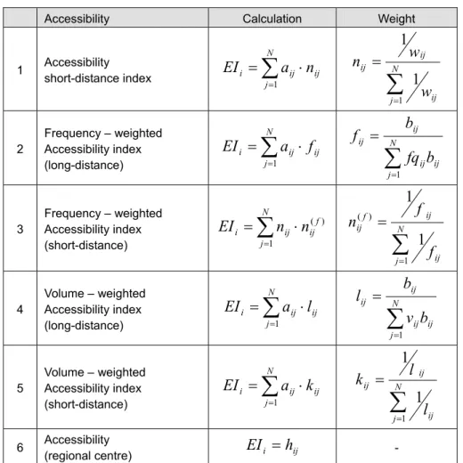
Table 1 shows the different accessibility indices based on different weighting schemes, which we will be used in the EAR model class. Note that long-distance indices use distances as weights while the local accessibility indices are calculated with the inverse weights of the long-distance accessibility indicator.

Table 1: Summary of weighted Accessibility Indicators

Accessibility Calculation Weight

1 Accessibility

short-distance index ∑

=

⋅

=

j

ij ij

i

a n

EI

1

∑

=

=

j ij

ij ij

w n w

1

1 1

2

Frequency – weighted Accessibility index

(long-distance) ∑

=

⋅

=

j ij ij

i

a f

EI

1

∑

=

=

j

ij ij ij ij

b fq f b

1

3

Frequency – weighted Accessibility index

(short-distance) ∑

=

⋅

=

j

f ij ij

i

n n

EI

1

) (

∑

=

j ij

f ij ij

f n f

1 ) (

1 1

4

Volume – weighted Accessibility index

(long-distance) ∑

=

⋅

=

j ij ij

i

a l

EI

1

∑

=

=

j ij ij ij ij

b v l b

1

5

Volume – weighted Accessibility index

(short-distance) ∑

=

⋅

=

j

ij ij

i

a k

EI

1

∑

=

=

j ij

ij ij

l k l

1

1 1

6 Accessibility

(regional centre) EI

= h

- Legend: fq ij ..is the train frequency between region i and region j, v

...goods volume between i and j (Railways)

Source: IHS.

∑

⋅

=

j ij ij

i

a w

EI

1

∑

=

=

j ij

ij

ij

b

w b

1

Apart from ordinary, frequency-weighted and volume-weighted indicators a further indicator was constructed to capture to connection between a centre of a larger region, which in our case are the capitals of NUTS-2 regions. For Lower Austria and the Burgenland two different sets of this indicator were calculated, either using the respective capitals of the states (Bundesland) or using Vienna as a central location in Austria.

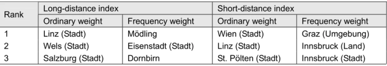
Table 2 displays the Austrian top 3 regions according to various accessibility indicators. With regards to the long-distance indicators we see that regions along the east western corridor are best accessible especially from more distant regions. Also, taking frequencies into account, we see that also regions from eastern Austria are among the best accessible regions.

With respect to local, a different picture emerges. Vienna and Linz as central locations of urban areas are ranked top. The frequency-weighted accessibility indicators on the other hand point to areas surrounding central cities.

Table 2: The top 3 political districts according to different accessibility indices Long-distance index Short-distance index

Rank

Ordinary weight Frequency weight Ordinary weight Frequency weight

1 Linz (Stadt) Mödling Wien (Stadt) Graz (Umgebung)

2 Wels (Stadt) Eisenstadt (Stadt) Linz (Stadt) Innsbruck (Land)

3 Salzburg (Stadt) Dornbirn St. Pölten (Stadt) Innsbruck (Stadt)

1 The model

1.1 The structure of the EAR model

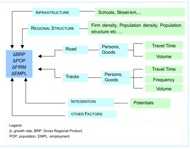
Figure 1 summarizes the structure of the EAR model. Regional growth is a function of infrastructure, regional structure, integration of regions, and traffic related accessibility.

Figure 1: Structure of the EAR model

Infrastructure is an important factor for economic growth and development of a region. A well-developed infrastructure ensures mobility of production factors within and across economies and should lead to a more efficient allocation and utilization of resources.

Demographic structures are an important determinant for regional developments, as e.g. in regions with an older population we cannot expect a high population growth. Another feature of the regional structure is the firm and population density. On average the prices of land in a region that is more densely populated will be higher. As a consequence the costs of establishing a firm will be higher in more densely populated areas.

ΔBRP ΔPOP ΔFIRM ΔEMPL

I

Road

Tracks

Schools, Street-km,...

I

Potentials

OTHER

F

Persons, Goods Persons, Goods

Travel Time Volume Travel Time

Frequency Volume R

S

Firm density, Population density, Population

structure etc. ...

Legend:

Δ: growth rate, BRP: Gross Regional Product, POP: population, EMPL: employment

As the role of accessibility was discussed in the previous section it will not be described further here.

The potentials of a region have to be incorporated in the model, as these variables influence either directly or indirectly the economic attractiveness of a particular region. Potentials are based on the gravitational formula of Newton. Bigger masses (or in economic analogy:

population, GRP, etc.) are more attractive than smaller masses relative to the distance of their barycentres. The economic barycentre can be the administrative and/or economic centres of regions.

The concept of potential variables can be extended to growth rates and are defined as follows:

Let dist

be the distance between the economic barycentres of regions i and j. The growth potential of region i with respect to region j or vice versa is defined as

j dist i

growth j growth i

j Potential i

, ,

= ⋅ , where i,j = 1,...,n.

From the equation above it can be seen that the potential variable depends inversely on the distance between the barycentres and positively on either one of the both growth rates. The distance variable can be interpreted also as a discount factor. In the EAR model various forms of distances are being considered, which can be either train or road travel times or coordinate distances.

1.2 Estimation results of the EAR model

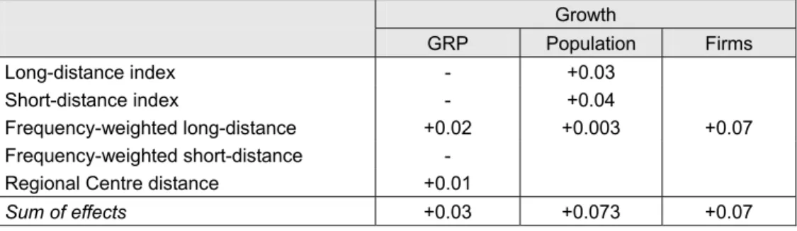
From the econometric estimation of the EAR model the following elasticities with respect to accessibilities were obtained:

Table 3: Elasticities of Regional Growth with respect to accessibility (Railroad) Growth

GRP Population Firms Long-distance index - +0.03

Short-distance index - +0.04

Frequency-weighted long-distance +0.02 +0.003 +0.07 Frequency-weighted short-distance -

Regional Centre distance +0.01

Sum of effects +0.03 +0.073 +0.07

Source: own estimation.

For economic growth two types of elasticities are important. On the one hand the frequency- weighted long-distance accessibility indicator influences the growth of the gross regional product and on the other hand we observe that accessibility with respect to the regional centre matters for regional growth. If both indicators are improved by one percent then regional growth will increase by 0.03 percent per year.

With regard to population growth, the ordinary long- and short-distance accessibility indicators affect population growth considerably. In addition, the frequency-weighted long- distance indicator affects population growth. In total this yields an overall elasticity with respect to accessibility of about 0.073 per year.

Firm growth also appears to be influenced by railroad accessibilities, in particular by the frequency-weighted long-distance accessibility indicator. An increase of this indicator by one percent increases regional firm growth by about 0.07 percent.

Employment effects could not be estimated econometrically as the elasticities of the models never appeared to be significant. This seems to be a problem of data measurement and will be explored in more details in future work. As a consequence we obtained employment predictions that are based on average firm size, multiplying average firm size with estimated firm growth.

2 Evaluation of four railroad infrastructure investment projects

Based on the estimated elasticities and future accessibility indicators we can now use this information to evaluate four infrastructure projects with the EAR model. The base year for our projections is 2003 – this was the last year for which we could obtain regional data. So we assume that in 2003 all new projects could have been realised and we compute the additional growth for the subsequent ten years – pretending that the traffic projects were already in operation. We obtain positive growth results for all four investment projects. Maps of regional growth patterns are shown in the appendix.

2.1 Project: The “Semmering Basistunnel” (old proposal)

The aim of the construction of the Semmering tunnel is to reduce travelling time from the northeast of Austria to the south of Austria by about 30 minutes.

4 We assumed that within the ten years forecast horizon. The firm sizes of new firms would be roughly equal to the size of the existing firms.

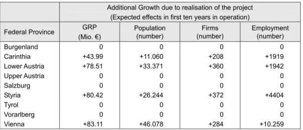
Table 4 displays the effects if the Semmering Basistunnel would be ten years in operation. It can be seen that the induced additional growth in Lower Austria, Styria and Vienna are of about the same size, whereas in Carinthia the effects are positive but smaller.

With regard to population growth Vienna would benefit most from the project.

Concerning the creation of new firms north eastern Styria would benefit most from the improved connection to Lower Austria and Vienna, and as well to central European markets.

Growth effects can be seen for regions north of the tunnel as well, since firms in Lower Austria would grow. This positive growth is also reflected in the employment predictions.

Table 4: Additional growth effects of the Semmering Basistunnel (old proposal) Additional Growth due to realisation of the project

(Expected effects in first ten years in operation) Federal Province GRP

(Mio. €)

Population (number)

Firms (number)

Employment (number)

Burgenland 0 0 0 0 Carinthia +43.99 +11.060 +208 +1919 Lower Austria +78.51 +33.371 +360 +1942

Upper Austria 0 0 0 0

Salzburg 0 0 0 0

Styria +80.42 +26.244 +372 +4404

Tyrol 0 0 0 0

Vorarlberg 0 0 0 0

Vienna +83.11 +46.078 +284 +10.259

2.2 Project 2: The Selzthal Bypass

This project is to bypass the regional town of Selzthal (in Upper Styria) for trains coming from the west (like Salzburg or Innsbruck) and going southeast (Graz). This would lead to a reduction in travelling times of about 7 Minutes.

Table 5 displays the main results of the EAR model for the Selzthal Bypass. Because regions

in the west and southeast of Austria become better connected, growth effects in all four

variables can be observed along this traffic axis. Regions in Styria benefits most, as well as

Tyrol and Salzburg, which come second in growth. We can even see some modest growth

effects for the far west region of Vorarlberg. Again, the better connection to the west Austrian

markets will be beneficial for firm growth in Styria.

Table 5: Additional growth effects of the Selzthal Bypass

Additional growth due to realisation of the project (Expected effects in first ten years in operation) Federal Province GRP

(Mio. €)

Population (number)

Firms (number)

Employment (number)

Burgenland 0 0 0 0

Carinthia 0 0 0 0

Lower Austria 0 0 0 0

Upper Austria 0 0 0 0

Salzburg +2 +1.320 +12 +98

Styria +9 +3.428 +35 +390

Tyrol +2.23 +1.270 +11 +91

Vorarlberg +1.09 +539 +5 +45

Vienna 0 0 0 0

Source: IHS EAR model-calculations.

2.3 Project 3: Mariazellerbahn

The Mariazellerbahn project envisages a change of the track width from narrow to standard gauge, but only for half of the present railroad line, which is a trunk line. This would improve travelling times up to 20 Minutes and will be combined with an increase in the train frequency.

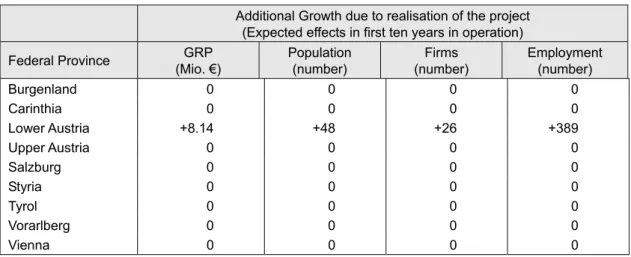
Table 6 displays the prediction results for the Mariazellerbahn project. As only two political districts are affected we only see some modest growth effects. Note that this project affects only regions in the federal state of Lower Austria.

Table 6: Additional growth effects of the Mariazellerbahn project

Additional Growth due to realisation of the project (Expected effects in first ten years in operation) Federal Province GRP

(Mio. €)

Population (number)

Firms (number)

Employment (number)

Burgenland 0 0 0 0

Carinthia 0 0 0 0

Lower Austria +8.14 +48 +26 +389

Upper Austria 0 0 0 0

Salzburg 0 0 0 0

Styria 0 0 0 0

Tyrol 0 0 0 0

Vorarlberg 0 0 0 0

Vienna 0 0 0 0

Source: IHS EAR model-calculations.

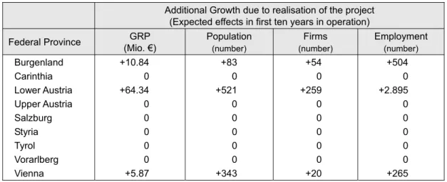
2.4 Project 4: Stadlau-Marchegg

The aim of the Stadlau-Marchegg project is basically an increase in train frequency between Vienna and Bratislava together with a shortening of travel time between the two cities of about 10 minutes.

Table 7: Additional growth effects of the Stadlau-Marchegg project Additional Growth due to realisation of the project

(Expected effects in first ten years in operation) Federal Province GRP

(Mio. €)

Population

Firms

Employment

Burgenland +10.84 +83 +54 +504

Carinthia 0 0 0 0

Lower Austria +64.34 +521 +259 +2.895 Upper Austria 0 0 0 0

Salzburg 0 0 0 0

Styria 0 0 0 0

Tyrol 0 0 0 0

Vorarlberg 0 0 0 0

Vienna +5.87 +343 +20 +265

Source: IHS EAR model-calculations.

Table 7 shows the effects of the project Stadlau-Marchegg. It can be seen that regions in the two federal states, Lower Austria and Vienna, will benefit from the improvement of accessibility vis-à-vis Bratislava. The far largest effect on the establishment of new firms can be seen for Lower Austria, some moderate effects for Burgenland and Vienna. This coincides with the additional growth patterns for GRP and employment.

3 Effects of the project on structurally weak regions

3.1 Classification of structurally weak regions

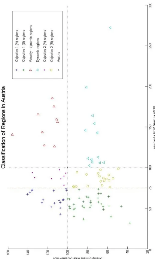
The classification of structurally weak regions is done along two variables: regional unemployment and per-capita gross regional product (GRP_pc). This classification of regions is based on the forecasts of Austrian households by the OEROK (Austrian regional planning conference).

We like to apply the EU structural fund classification method of objective 1 and 2 regions to

find out if weak regions might benefit from the investment projects. This method of

classification has the advantage of comparing the regional economic classification method of

the EU for Austrian regions. Objective 1 regions of the European structural fund are

characterised by their relative regional economic performance. Objective 1 regions are those, where the gross domestic product is below 75 % of the Community average.

We furthermore define an objective 2 group that consists of regions that have a per-capita GRP between 75 % and 100 % of the Austrian average.

The second important variable for our classification is the unemployment rate.

The table with all the classification results for political districts can be found in the appendix.

We lie to concentrate the discussion on five groups of regions that are defined as follows:

1. The objective 1 (A) group: regions with high unemployment (17)

Regions in this class are characterised by a very small per-capita GRP and a high unemployment rate, which is above average. Within these regions there are 12 % of the Austrian population and it accounts for about 7.7 % of Austrian GRP. Furthermore, there are 11 % of all firms and 14 % of total employment.

2. The objective 1 (B) group: regions with unemployment below average (33)

These regions have a per-capita GRP far below average and unemployment below average. Within these regions there are 22.5 % of the Austrian population and it accounts for about 12.6 % of Austrian GRP. Furthermore, in this group there are 17.8 % of all firms and 21.3 % of total employment.

3. Objective 2 regions (27)

Objective 2 regions are those with a per-capita GRP between 75 % and 100 % of the Austrian average. These regions can be further subdivided into an objective 2 (A) group (unemployment above average) and an objective 2 (B) group (unemployment below average). Within the objective 2 regions there are 24.3 % of the Austrian population and they account for about 21.2 % of Austrian GRP. Furthermore, there are 24.1 % of all firms in this group that have 33.1 % of total employment.

4. Weakly dynamic regions (9)

These regions are characterised by having a per-capita GRP above the average and at the same time an unemployment rate above the average. These are mostly regions with larger towns in Austria and they account for 27.1 % of the total population, 38.4 % of total GRP, 29.8 % of all firms, and 18.6 % of total employment.

5 The basis for the calculation of relative economic performance here is the Austrian per-capita GRP in contrast to the Community average.

6 The definition of the unemployment rate departs from the conventional definitions. It was not available at the level of political districts. Instead we divided the number of unemployed by the potential labour force per district, i.e. the number of people between 15 and 65 years of age.

5. Dynamic regions (13)

Dynamic regions are those regions with a per-capita GRP above the average and an unemployment rate below the average. Their share of the Austrian population is about 14 %, the GRP share is about 20 %. In these regions there are 17.2 % of all Austrian firms, but only 12.3 % of total employment. This shows that these regions have also a high productivity.

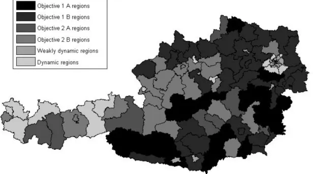
Figure 2: Classification of Austrian Regions

Figure 2 shows the classification of 99 Austrian regions by a map:

Figure 3: Classification of Austrian regions (2)

Source: IHS.

3.2 Effects of infrastructure projects on structurally weak regions

3.2.1 Project 3: Semmering Basistunnel

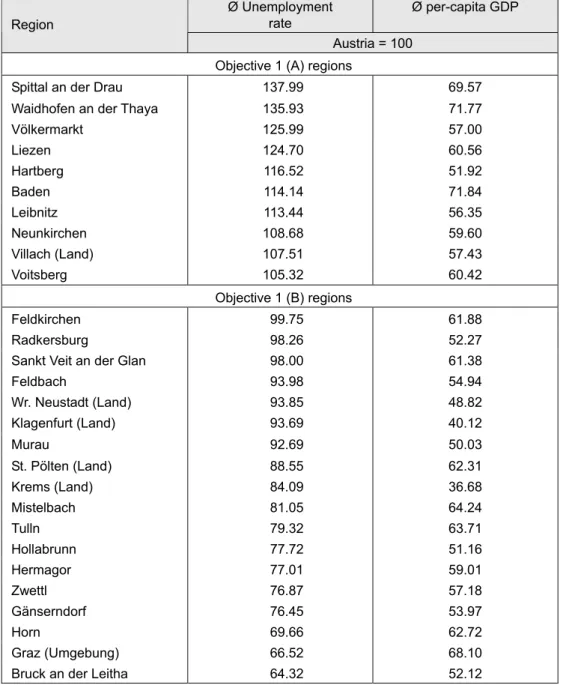
The Semmering tunnel project affects most of structurally weak regions of Austria. Table 8 shows theses regions classified into Objective 1 and 2 groups.

Table 8: Objective 1 regions that will benefit from the Semmering Basistunnel Ø Unemployment

rate

Ø per-capita GDP Region

Austria = 100 Objective 1 (A) regions

Spittal an der Drau 137.99 69.57 Waidhofen an der Thaya 135.93 71.77

Völkermarkt 125.99 57.00

Liezen 124.70 60.56

Hartberg 116.52 51.92

Baden 114.14 71.84

Leibnitz 113.44 56.35

Neunkirchen 108.68 59.60

Villach (Land) 107.51 57.43

Voitsberg 105.32 60.42

Objective 1 (B) regions

Feldkirchen 99.75 61.88

Radkersburg 98.26 52.27

Sankt Veit an der Glan 98.00 61.38

Feldbach 93.98 54.94

Wr. Neustadt (Land) 93.85 48.82 Klagenfurt (Land) 93.69 40.12

Murau 92.69 50.03

St. Pölten (Land) 88.55 62.31 Krems (Land) 84.09 36.68

Mistelbach 81.05 64.24

Tulln 79.32 63.71

Hollabrunn 77.72 51.16

Hermagor 77.01 59.01

Zwettl 76.87 57.18

Gänserndorf 76.45 53.97

Horn 69.66 62.72

Graz (Umgebung) 66.52 68.10

Bruck an der Leitha 64.32 52.12

10 from 17 objective 1 regions will benefit from the project, which are about 60 % of all regions. For the objective 1 (B) regions the share of affected regions is about 55 %.

3.2.2 Selzthal Bypass

Table 9 shows that only 18 % of all objective 1 (A) and 6 % of all objective 1 (B) are affected by the project. All those regions are parts of the federal province of Styria, as the western parts of Austria tends to be more dynamic with respect to the indicators chosen to classify the regions.

Table 9: Affected objective 1 regions (Selzthal Bypass) Ø Unemployment

rate

Ø per-capita Region GDP

Austria = 100 Objective 1 (A) regions

Hartberg 116.52 51.92

Leibnitz 113.44 56.35

Voitsberg 105.32 60.42

Objective 1 (B) regions

Feldbach 93.98 54.94

Graz (Umgebung) 66.52 68.10

3.2.3 Project 4: Stadlau – Marchegg

As this project has only local effects the reference per-capita GDP as well as the reference unemployment rate are the ones of the three most eastern provinces, Lower Austria, Vienna and the Burgenland.

As seen from the table below, 1 out of the two objective 1 (A) regions and 17 out of 23

objective 1 (B) region might benefit from the project.

Table 10: Affected objective 1 regions (Stadlau – Marchegg) Ø Unemployment

rate

Ø per-capita Region GDP

Vie+LOAT*+BGLD = 100 Objective 1 (A) regions

Waidhofen an der Thaya 112.49 66.21 Objective 1 (B) regions

Baden 94.46 66.27

Neunkirchen 89.93 54.98 Wr. Neustadt (Land) 77.66 45.03

St. Pölten (Land) 73.28 57.48

Mattersburg 73.27 67.47

Lilienfeld 69.87 53.80

Krems (Land) 69.59 33.84

Mistelbach 67.07 59.26

Tulln 65.64 58.77

Hollabrunn 64.32 47.20

Zwettl 63.61 52.74

Gänserndorf 63.27 49.79

Horn 57.64 57.86

Scheibbs 57.22 62.82

Melk 57.17 53.23

Amstetten 54.10 72.42 Bruck an der Leitha 53.23 48.08

Source: IHS calculations. * LOAT = Lower Austria.

3.2.4 Effectiveness of projects with respect to structurally weak regions

Figures 4 and 5 display the effects of the four projects on the regions, which were clustered according to the methodology described above. As can be seen for GDP per capita considerable part of the effects will be on structurally weak regions in case of the Semmering and Stadlau-Marchegg projects, especially on objective 1 (A+B) regions. For the Selzthal Bypass the effects concern mostly objective 2 regions with some big effects also for the better-developed regions. We also calculated the correlation coefficient between the generated additional GDP per capita in all regions and the GDP per capita index series (Austria=100). In case a project contributes a lot towards improving the GDP per capita the correlation coefficient would be close to -1. The Semmering Basistunnel displays a correlation coefficient of 0.08, which appears to be the best as well, followed by the Selzthal Bypass (0.15) and the Stadlau-Marchegg project (0.3). The Mariazell project displays a correlation coefficient of about 0.22.

As far as improvement of the unemployment situation is concerned (compare figure 5) some

effects can be expected from the Selzthal Bypass and Stadlau-Marchegg projects, but most

jobs will be created in regions of high unemployment due to the Semmering Basistunnel. We also calculated the correlation coefficient for this purpose, which now changes in meaning.

An ideal project would now display a correlation coefficient of +1, because in this case most of the jobs would be created in regions with a high unemployment rate. According to our calculations we find a correlation coefficient between additional jobs and the unemployment rate index of about 0.32 for the Semmering Basistunnel, 0.18 for the Stadlau-Marchegg project and 0.06 for the Selzthal Bypass. The Mariazell project displays a correlation coefficient of about 0.1.

Figure 4: Change in GDP per capita and structurally weak regions

Figure 5: The creation of new jobs in structurally weak regions

4 Comparative ranking of the projects

To compare the individual projects we aggregate the regional effects for the total Austrian economy. These are shown in Table 11:

Table 11: Ranking of the projects according to their economic effects over 10 years of operation

Target

Cumulated growth (First ten years in operation) Rank Project

BRP (Mio. €)

Population (number)

Firms (number)

Employment (number) 1 Semmering

Basistunnel (old plan) +286.03 +116.753 +1.224 +18.524 2 Stadlau – Marchegg +81.05 +947 +333 +3.664 3 Selzthal Bypass +14.29 +6.557 +63 +624 4 Mariazellerbahn +8.14 +48 +26 +389

a. GRP – Effects

The effects on GRP are largest for the Semmering Basistunnel project, followed by Stadlau – Marchegg, the Selzthal Bypass, and the Mariazellerbahn project. This ranking is not surprising; it shows the projects that have the largest regional diffusions.

b. Population effects

As far as population growth is concerned we see the largest effects stems from the Semmering project, followed by the Selzthal Bypass, Stadlau – Marchegg, and Mariazellerbahn.

c. Firm effects

Concerning firm growth we see the largest effects for the Semmering Basistunnel.

About a quarter of this new number of firms would be created in case of the Stadlau – Marchegg project, and about 60 new firms would be set up in the first ten years of the operation of the Selzthal bypss and less than 30 in case of the Mariazellerbahn.

d. Employment effects

Regarding employment we see that of course the ranking has not changed vis-à-vis

the additional firm growth. The by far largest effect could be seen for the Semmering

Basistunnel with about 18,000 newly employed people. For the Stadlau – Marchegg

project about 3,600 new jobs would be created. For the Selzthal bypass the model

projects the creation of about 600 new jobs and for the Mariazellerbahn less than 400 in the first ten years of operation.

e. Indexation and ranking

Table 12 displays the ranking of the projects in form of a weighted and ordinary average ranking. It is not surprising that Semmering-Basistunnel appears to be the best according to the target criteria. As seen before, the worst ranking can be found for the Mariazellerbahn. As regards to the average rank, the Stadlau – Marchegg is slightly ahead of the Selzthal bypass. Thus, the EAR model leads to clear ranking of the 4 projects:

Table 12: Indexation for the ranking according to four economic target variables Target Criteria

(Rank numbers) Rank Avg.

Rank

Weighted

Rank

Project

GRP

(Rank)

Population (Rank)

Firms (Rank)

Employment (Rank) 1 1.0 1.0 Semmering

Basistunnel (old) 1 1 1 1 2 2.25 2.2 Stadlau – Marchegg 2 3 2 2 3 2.75 2.8 Selzthal Bypass 3 2 3 3 4 4.0 4.0 Mariazellerbahn 4 4 4 4

5 Summary

In this paper we have developed a modelling and ranking strategy for the evaluation of infrastructure and related projects based on the concept of accessibility. This model – as shown – can produce results for various levels of aggregation and enables the user to pin down geographically effects of projects to be undertaken for various variables she is interested in.

We then successfully applied this evaluation model to four investment projects of the Austrian federal railways, the Semmering Basistunnel, the Selzthal bypass, the Mariazellerbahn and the Stadlau – Marchegg project. It was shown that the regional and national economic effects of these projects vary considerably in scope and magnitude.

Eventually, based on the 10-year EAR predictions, a comparative ranking was the final result to assess all four projects.

7 The following weights were used 3:2:2:3 = GRP:POP:FIR:EMPL.

References

Baldwin R., Forslid R., Martin P., Ottaviano G., Robert-Nicoud F. (2003): Economic Geography and Public Policy. Princeton University Press, Princeton and Oxford.

Baldwin R. and Krugman P. (2004): Agglomeration, integration, and tax harmonisation.

European Economic Review 48, pp. 1-23.

Barro R. and Sala-i-Martin X. (1995): Economic Growth. McGraw Hill, New York.

Kakamu K., Polasek W., and Wago H. (2006): Bayesian seemingly unrelated regression in spatial regional models: Economics of agglomeration in Japan during 1991-2000, mimeo (paper presented at the 8th Valencia Meeting).

Krugman P. (1991): Increasing Returns and Economic Geography. Journal of Political Economy 99 (2), pp. 843-499.

ÖROK (2005): ÖROK-Prognosen 2001-2031, Teil 2: Haushalte und Wohnungsbedarf nach Regionen und Bezirken Österreichs. ÖROK Schriftenreihe 166/2, Wien.

Polasek W. (2005): Improving Train Network until 2020: A stimulus for regional growth? IHS Wien, mimeo.

Polasek W. and Berrer H. (2005a): Regional Growth in Central Europe: Long-term effects of population structure. IHS Wien, mimeo.

Polasek W. and Berrer H. (2005b): Infrastructure and GDP growth in Central European Regions. IHS Wien, mimeo.

Polasek W. and Berrer H. (2005c): Regional Growth modelling and traffic accessibility. IHS Wien, mimeo.

Polasek W. und Sellner R. (2005): Ost-West Benchmarking: Die Stellung österreichischer

Regionen in Zentraleuropa. Projektbericht 40.169, IHS Wien.

Appendix A: Maps displaying the regional effects of the investment projects

Figure 6: Semmering Basistunnel

Growth of GRP

Firm growth

Population Growth

Figure 7: Selzthal Bypass

Growth of GRP

Population Growth

Firm Growth

Figure 8: Mariazellerbahn

Legend:

Black: St. Pölten (Land): +0.003 % Grey: St. Pölten (Stadt): +0.004 %

Growth of the Gross Regional Product

Population Growth

Firm Growth

Legend:

Black: St. Pölten (Land): +0.054 % Grey: St. Pölten (Stadt): +0.080 %

Legend:

Black: St. Pölten (Land): +0.016 % Grey: St. Pölten (Stadt): +0.023 %

Figure 9: Stadlau – Marchegg

Growth of GRP

Population Growth

Firm Growth

Appendix B: Classification of structurally weak regions

B.1 Austria

Table 13: Objective 1 (A) regions

Ø Unemployment rate

Ø per-capita Region GDP

Austria = 100

Rust (Stadt) 107.35 50.45

Güssing 107.41 42.64

Oberpullendorf 104.16 60.52

Oberwart 140.40 67.33

Spittal an der Drau 137.99 69.57 Villach (Land) 107.51 57.43

Völkermarkt 125.99 57.00

Wolfsberg 100.98 72.09

Baden 114.14 71.84

Neunkirchen 108.68 59.60

Waidhofen an der Thaya 135.93 71.77

Hartberg 116.52 51.92

Leibnitz 113.44 56.35

Liezen 124.70 60.56

Mürzzuschlag 101.82 74.31

Voitsberg 105.32 60.42

Lienz 135.80 72.83

Source: own calculations.

Table 14: Objective 1 (B) regions

Ø Unemployment rate

Ø per-capita GDP Region

Austria = 100

Eisenstadt (Umgebung) 83.58 50.89

Jennersdorf 97.87 49.64

Mattersburg 88.53 73.14

Neusiedl am See 85.11 52.89

Hermagor 77.01 59.01

Klagenfurt (Land) 93.69 40.12 St. Veit an der Glan 98.00 61.38

Feldkirchen 99.75 61.88

Bruck an der Leitha 64.32 52.12

Gänserndorf 76.45 53.97

Hollabrunn 77.72 51.16

Horn 69.66 62.72

Krems (Land) 84.09 36.68

Lilienfeld 84.43 58.32

Melk 69.09 57.71

Mistelbach 81.05 64.24

St. Pölten (Land) 88.55 62.31

Scheibbs 69.14 68.09

Tulln 79.32 63.71

Wr. Neustadt (Land) 93.85 48.82

Zwettl 76.87 57.18

Braunau am Inn 69.04 73.72

Eferding 46.11 52.62

Freistadt 56.65 39.73

Grieskirchen 59.06 64.44

Rohrbach 58.60 52.96

Schärding 66.30 55.53

Steyr (Land) 64.14 48.68 Urfahr (Umgebung) 37.60 31.77

Feldbach 93.98 54.94

Graz (Umgebung) 66.52 68.10

Murau 92.69 50.03

Radkersburg 98.26 52.27

Source: own calculations.

Table 15: Objective 2 regions

Ø Unemployment rate

Ø per-capita GDP Region

Austria = 100 Objective 2 (A) regions

Landeck 135.56 93.76

Gmünd 133.19 87.96

Bruck an der Mur 116.21 86.7

Judenburg 108.39 97.51

Imst 107.01 86.49

Fürstenfeld 103.85 89.69

Knittelfeld 103.74 78.42

Zell am See 101.95 93.3 Objective 2 (B) regions

Leoben 94.22 77.07

Tamsweg 94.06 76.2

Deutschlandsberg 91.46 76.85

Kitzbühel 90.76 94.53

St. Johann/Pongau 81.19 91.72

Weiz 79.92 77.42

Linz (Land) 69.33 93.05

Feldkirch 68.11 89.6

Korneuburg 67.17 97.41

Vöcklabruck 66.75 83.31

Amstetten 65.38 78.5

Wels (Land) 64.15 87.38 Ried im Innkreis 63.36 84.05

Gmunden 61.19 86.36

Hallein 58.67 91.3

Innsbruck (Land) 58.42 84.43

Perg 57.5 76.28

Kirchdorf an der Krems 54.54 87.06

Salzburg (Umgebung) 49.19 98.59

Table 16: Weakly dynamic regions

Ø Unemployment rate

Ø per-capita GDP Region

Austria = 100

Klagenfurt (Stadt) 110.08 156.59 Villach (Stadt) 125.58 143.66 Krems an der Donau (Stadt) 113.80 175.62 St. Pölten (Stadt) 115.50 185.50 Wr. Neustadt (Stadt) 123.73 127.58 Steyr (Stadt) 129.91 165.77 Wels (Stadt) 111.24 159.40 Graz (Stadt) 113.44 126.29 Wien (Stadt) 155.71 140.80

Table 17: Dynamic regions

Ø Unemployment rate

Ø per-capita Region GDP

Austria = 100

Eisenstadt (Stadt) 57.24 272.36 Waidhofen an der Ybbs (Stadt) 63.83 106.40

Mödling 70.37 142.90

Wien (Umgebung) 82.33 146.28 Linz (Stadt) 81.30 199.17 Salzburg (Stadt) 75.04 164.01 Innsbruck (Stadt) 73.35 154.52

Kufstein 67.76 105.88

Reutte 78.52 102.78

Schwaz 75.41 106.89

Bludenz 69.51 113.00

Bregenz 76.30 110.06

Dornbirn 79.65 111.41

Source: own calculations.

Figure 10: Share of Classes (Avg.: 1998:2003)

Source: own calculations.

B.2 Lower Austria, Vienna, and Burgenland

Table 18: Structurally weak regions in Lower Austria, Vienna, and Burgenland Ø Unemployment

rate

Ø per-capita Region GDP

Vienna+LOAT+Burgenland = 100 Objective 1 (A) regions

Oberwart 116.18 62.11

Waidhofen an der Thaya 112.49 66.21 Objective 1 (B) regions

Rust (Stadt) 88.83 46.54 Eisenstadt (Umgebung) 69.17 46.94

Güssing 88.89 39.34

Jennersdorf 80.99 45.79

Mattersburg 73.27 67.47

Neusiedl am See 70.43 48.79

Oberpullendorf 86.20 55.83

Amstetten 54.10 72.42

Baden 94.46 66.27

Bruck an der Leitha 53.23 48.08

Gänserndorf 63.27 49.79

Hollabrunn 64.32 47.20

Horn 57.64 57.86

Krems (Land) 69.59 33.84

Lilienfeld 69.87 53.80

Melk 57.17 53.23

Mistelbach 67.07 59.26

Neunkirchen 89.93 54.98

St. Pölten (Land) 73.28 57.48

Scheibbs 57.22 62.82

Tulln 65.64 58.77

Wr. Neustadt (Land) 77.66 45.03

Zwettl 63.61 52.74

Source: own calculations.

Table 19: Classification of regions in Vienna, Lower Austria and the Burgenland Ø Unemployment

rate

Ø per-capita Region GDP

Vienna+LOAT+Burgenland = 100 Weakly dynamic regions

Wr. Neustadt (Stadt) 102.39 117.69 Wien (Stadt) 128.86 129.89

Dynamic regions

Eisenstadt (Stadt) 47.37 251.25 Krems an der Donau (Stadt) 94.18 162.01 St. Pölten ( Stadt) 95.58 171.12

Mödling 58.23 131.82

Wien (Umgebung) 68.13 134.94 Objective 2 (A) regions

Gmünd 110.22 81.14

Objective 2 (B) regions

Waidhofen an der Ybbs (Stadt) 52.82 98.16

Korneuburg 55.59 89.86

Source: own calculations.

Figure 11: Shares of Classes (

Basis: Vienna, Lower Austria, Burgenland)

Source: own calculations.

Authors: Wolfgang Polasek, Wolfgang Schwarzbauer

Title: Traffic Accessibility and the Effect on Firms and Population in 99 Austrian Regions

Reihe Ökonomie / Economics Series 198

Editor: Robert M. Kunst (Econometrics)

Associate Editors: Walter Fisher (Macroeconomics), Klaus Ritzberger (Microeconomics)

ISSN: 1605-7996

© 2006 by the Department of Economics and Finance, Institute for Advanced Studies (IHS),

Stumpergasse 56, A-1060 Vienna • +43 1 59991-0 • Fax +43 1 59991-555 • http://www.ihs.ac.at

ISSN: 1605-7996