An Integrated CVaR and Real Options Approach to Investments in the Energy Sector

IHS Economics Series Working Paper 209

May 2007

An Integrated CVaR and Real Options Approach to Investments in the Energy Sector

Ines Fortin

Sabine Fuss

Jaroslava Hlouskova

Nikolay Khabarov

Michael Obersteiner

Jana Szolgayova

Impressum Author(s):

Ines Fortin, Sabine Fuss, Jaroslava Hlouskova, Nikolay Khabarov, Michael Obersteiner, Jana Szolgayova

Title:

An Integrated CVaR and Real Options Approach to Investments in the Energy Sector ISSN: Unspecified

2007 Institut für Höhere Studien - Institute for Advanced Studies (IHS) Josefstädter Straße 39, A-1080 Wien

E-Mail: o ce@ihs.ac.atffi Web: ww w .ihs.ac. a t

All IHS Working Papers are available online: http://irihs. ihs. ac.at/view/ihs_series/

This paper is available for download without charge at:

https://irihs.ihs.ac.at/id/eprint/1770/

209 Reihe Ökonomie Economics Series

An Integrated CVaR and Real Options Approach to Investments in the Energy Sector

Ines Fortin, Sabine Fuss, Jaroslava Hlouskova,

Nikolay Khabarov, Michael Obersteiner, Jana Szolgayova

209 Reihe Ökonomie Economics Series

An Integrated CVaR and Real Options Approach to Investments in the Energy Sector

Ines Fortin, Sabine Fuss, Jaroslava Hlouskova, Nikolay Khabarov, Michael Obersteiner, Jana Szolgayova May 2007

Institut für Höhere Studien (IHS), Wien

Institute for Advanced Studies, Vienna

Contact:

Ines Fortin

IHS, Stumpergasse 56, 1060 Vienna, Austria : 43/1/59991-165

Email: fortin@ihs.ac.at Sabine Fuss

University of Maastricht/UNU-Merit Keizer Karelplein 19, 6211 TC Maastricht, The Netherlands : +31/43/3884-430

email: S.Fuss@algec.unimaas.nl Jaroslava Hlouskova

IHS, Stumpergasse 56, 1060 Vienna, Austria : 43/1/59991-142

email: hlouskov@ihs.ac.at Nikolay Khabarov

International Institute for Applied Systems Analysis (IIASA) 2361 Laxenburg, Austria

: +43/2236/807-346 email: khabarov@iiasa.ac.at Michael Obersteiner

International Institute for Applied Systems Analysis (IIASA) 2361 Laxenburg, Austria

: +43/2236/807-460 email: oberstei@iiasa.ac.at Jana Szolgayova

International Institute for Applied Systems Analysis (IIASA) 2361 Laxenburg, Austria

: +43/2236/807-349 email: szolgay@iiasa.ac.at

Founded in 1963 by two prominent Austrians living in exile – the sociologist Paul F. Lazarsfeld and the economist Oskar Morgenstern – with the financial support from the Ford Foundation, the Austrian Federal Ministry of Education and the City of Vienna, the Institute for Advanced Studies (IHS) is the first institution for postgraduate education and research in economics and the social sciences in Austria.

The Economics Series presents research done at the Department of Economics and Finance and aims to share “work in progress” in a timely way before formal publication. As usual, authors bear full responsibility for the content of their contributions.

Das Institut für Höhere Studien (IHS) wurde im Jahr 1963 von zwei prominenten Exilösterreichern – dem Soziologen Paul F. Lazarsfeld und dem Ökonomen Oskar Morgenstern – mit Hilfe der Ford- Stiftung, des Österreichischen Bundesministeriums für Unterricht und der Stadt Wien gegründet und ist somit die erste nachuniversitäre Lehr- und Forschungsstätte für die Sozial- und Wirtschafts- wissenschaften in Österreich. Die Reihe Ökonomie bietet Einblick in die Forschungsarbeit der Abteilung für Ökonomie und Finanzwirtschaft und verfolgt das Ziel, abteilungsinterne Diskussionsbeiträge einer breiteren fachinternen Öffentlichkeit zugänglich zu machen. Die inhaltliche Verantwortung für die veröffentlichten Beiträge liegt bei den Autoren und Autorinnen.

Abstract

The objective of this paper is to combine a real options framework with portfolio optimization techniques and to apply this new framework to investments in the electricity sector. In particular, a real options model is used to assess the adoption decision of particular technologies under uncertainty. These technologies are coal-fired power plants, biomass- fired power plants and onshore wind mills, and they are representative of technologies based on fossil fuels, biomass and renewables, respectively. The return distributions resulting from this analysis are then used as an input to a portfolio optimization, where the measure of risk is the Conditional Value-at-Risk (CVaR).

Keywords

Portfolio optimization, CVaR, climate change policy, uncertainty, real options, electricity, investments

JEL Classification

C61, D81, D92, G11, Q4, Q56, Q58

Comments

Ines Fortin, Jaroslava Hlouskova, and Michael Obersteiner gratefully acknowledge financial support from the Austrian National Bank (Jubiläumsfonds Grant No. 11883).

AT IIASA this work was carried out in the framework of the project "Bewertungsmodelle für zukünftige Energiecluster unter Markt-,Technologie- und Politikunsicherheit - Fallstudie Biomasse" funded by FFG (Österreichische Forschungsförderungsgesellschaft), Vienna. Sabine Fuss, Nikolay Khabarov, Michael Obersteiner and Jana Szolgayova are grateful for the financial support of FFG.

Contents

1 Introduction 1

2 The Real Options Model 5

2.1 The Framework ... 5

2.2 The Technologies and the Data ... 9

2.3 Results of the Real Options Model ... 10

3 CVaR-based Portfolio Optimization 15

3.2 Portfolio Optimization: Minimizing Risk ... 17

3.3 Portfolio Optimization: Maximizing Returns ... 18

3.4 Results of the CVaR Approach ... 19

3.5 Mean-variance versus CVaR ... 23

4 Conclusion 27

Appendix A: Snapshots of Price Distributions for All Scenarios 29 Appendix B: Real Options Output for Investing and Switching 30 Appendix C: Definitions of Copulas and Related Concepts 33

References 35

1 Introduction

Uncertainty about the cause-and-effect relationships of anthropogenic emissions, global warm- ing and a large number of (possibly irreversible) effects impedes effective policy making and poses considerable uncertainties to investors in addition to the common uncertainties origi- nating from fluctuations in input and output prices. If investors cannot be sure about future climate change policy measures, they will typically not invest in environmentally friendly, expensive technologies. Therefore, it is important not only to concentrate on variability in returns from market-driven fluctuations in prices, but also to take into account the uncer- tainties emanating from the policy making process. In this paper we will focus on investment planning in the electricity sector, since the generation of electricity contributes significantly to total CO

emissions and has therefore been a major area of concern to policymakers.

The electricity sector is marked not only by uncertainties surrounding investment and production decisions, but also by irreversibility due to the large sunk costs involved in invest- ment in generation equipment and the flexibility to postpone investments to a later point in time during the planning horizon. Therefore, we think that real options modeling is a suitable approach for investment planning. Originally developed for valuing financial options in the seventies (Black and Scholes, 1973, and Merton, 1973), economists soon realized that option pricing also provided considerable insight into decision-making concerning capital investment.

Hence the term “real” options. Early frameworks were developed by McDonald and Siegel (1986), Pindyck (1988, 1991, 1993), and Dixit and Pindyck (1994).

The basic idea is that standard investment theory relying on net present value (NPV) calculations generally do not consider the interaction between three important characteristics of investment decisions: the irreversibility of most investments, which implies that a substantial portion of the total in- vestment cost is sunk, the uncertainty surrounding the future cash flows from the investment, which can be affected by e.g. the volatility of output and input prices, and the opportunity of timing the investment flexibly. Regarding the opportunity to defer an investment means that we can assign a value to waiting. In other words, investors gain more information about the uncertainty that surrounds economic decisions as time passes by. Therefore, staying flexible by postponing decisions has an option value if the degree of uncertainty faced is big enough.

This value increases if the sunk cost that has to be incurred to launch the project is high, but also in times of larger uncertainty associated with future cost or revenues. In this case it pays off to wait and see how the conditions have changed, especially if they are expected to be rather stable afterwards.

Investment in the electricity sector has been analyzed within real options frameworks before. In the area of short-term planning, this work includes e.g. Tseng and Barz (2002), Hlouskova et al (2005) and Deng and Oren (2003). At the same time, a number of long- term planning frameworks have emerged. A recent example is by Fleten et al (2006), who find that investment in power plants relying on renewable energy sources will be postponed beyond the traditional NPV break even point when a real options approach with stochastic electricity prices is used. With respect to uncertainty from government regulation in the electricity sector, De Jong et al (2004) propose that real options modeling is a valuable method to investigate how fluctuations in future emissions prices affect investment patterns. Also Laurikka (2004), Laurikka and Kojonen (2006), Kiriyama and Suzuki (2004), and Reedman

1For a comprehensive treatment and overview of both financial and real options theory see Trigeorgis (1996). More advanced and with several applications is Schwartz and Trigeorgis (2001).

et al (2006) deal with the influence of future uncertain emissions trading and with CO

penalties within a real options setup. In these models the design of emissions trading schemes and the number of allowances that are freely distributed are main features of the overall model.

On the other hand, Fuss et al (2006) focus on the overall effect of uncertainty emanating from climate change policy and the effect of market uncertainty, where the specific form of emissions trading schemes is not an issue. In their framework CO

prices can be seen as a sort of carbon tax or as the price for an allowance that has to be bought on the carbon market;

CO

prices thus add to the total cost of electricity producers. We use this same framework in the present paper. Sources of uncertainty are the price of CO

and the price of electricity, which are modeled as stochastic processes. A feature of the model which is disregarded in many other frameworks is the relation between CO

costs and electricity prices. In our model this is captured by the fact that the increments of the two price processes and thus the price processes themselves are positively correlated. In fact the use of (linear) correlation to describe and model dependence implies a symmetric dependence structure. To capture the intuitively plausible fact that dependence may be higher in times of increasing prices than in times of decreasing prices, more general forms of dependence modeling involving so-called copulas would be appropriate. Solving this is beyond the scope of our paper and will be left for future research.

We use a real options model to find the optimal timing of investing into carbon capture and storage (CCS) modules in the case of coal- and biomass-fired power plants. For renewables the optimal installation time of the plant as such is computed. We find that the wind turbine, the basic coal plant (without CCS) and the basic biomass plant (without CCS) are all built in the first year.

While this optimization is performed by the individual power producer, who wants to set up a new plant, large investors would typically want to invest in a portfolio of technologies rather than concentrate on a single technology or a single chain. The contribution of this paper is to combine portfolio optimization with the results that we derive from our real op- tions framework. In particular, we use the real options model to find the optimal investment strategy and its implied return distributions; the return distributions, then, can be employed as an input into the portfolio optimization. In traditional finance, the standard portfolio op- timization procedure is the mean-variance approach introduced by Markowitz (1952), where the portfolio variance is minimized subject to a constraint on the expected return. Risk man- agement in financial institutions, however, has started to employ another measure of risk, the Value-at-Risk (VaR), since it captures extreme – and thus dangerous – events providing information on the tail of a distribution. Also regulatory requirements as specified by the Basel Committee on Banking Supervision (2003, 2006) are geared towards the use of VaR.

Another risk measure, which is closely related to VaR but offers additional desirable prop- erties like coherence and computational ease, is Conditional Value-at-Risk (CVaR). While VaR is generally better known and more widely employed, we think that CVaR is the more appropriate measure to use. Let us define VaR and CVaR to make clear what we are talking about. According to Rockafellar and Uryasev (2000) the β-VaR of a portfolio is the lowest amount α such that, with probability β, the loss will not exceed α, whereas the β-CVaR is the conditional expectation of losses above that amount α, where β is a specified probability level.

2This (simple) definition applies only to situations where the loss distribution is continuous. For the

The disadvantages of VaR as opposed to CVaR relate to both usefulness in risk manage- ment and technical properties. VaR does not consider losses exceeding the threshold value while CVaR does, and this information might be useful, in particular in times of financial distress. Further, VaR is only a coherent risk measure in the sense of Artzner et al (1999) if distributions are assumed to be normal; generally, VaR is neither subadditive nor convex.

CVaR, on the other hand, is always a coherent risk measure. In addition, the powerful results in Rockafellar and Uryasev (2000, 2002) make computational optimization of CVaR readily accessible. Note that, under mild technical restrictions, the minimization of VaR and CVaR and the mean-variance framework yield the same results provided that all underlying distri- butions are normal. This does not apply if the assumption of normality is violated. We will see that both the univariate distributions and the joint distribution (copula) of the returns, which are the results from our real options procedure, do not seem to be normal in most cases. A more detailed treatment of the difference between VaR and CVaR can be found in Rockafellar and Uryasev (2000). To our knowledge, combining real options with portfolio optimization using CVaR is a new approach which has not been implemented before. Some recent literature has undertaken steps into similar directions, however.

Alesii (2005) uses VaR in combination with real options, but his aims and therefore also his approach are very different from ours. He acknowledges that with a real options approach downside risk is reduced and the distribution of the expanded NPV

is thus favorably skewed (Trigeorgis, 1996). The aim of his paper is to quantify this impact on risk. To this end he uses an extension of the model by Kulatilaka (1988) to calculate the VaR on the expanded NPV and the CFaR (the cash-flow-at-risk in each period of the planning horizon). To be more precise, he first derives expanded NPVs and optimal exercise thresholds for all options with backward induction. Then, with a stochastic, mean-reverting state variable, he conducts a Monte Carlo simulation and uses the simulated time series to compute the cash flows considering the optimal exercise times. Alesii (2005) calls these cash flows “controlled” cash flows and uses them to calculate the expanded NPVs, which converge to the values previously computed recursively. The model results confirm that real options reduce downside risk and reshape the distribution of the expanded NPV positively: Both VaR and CFaR decrease substantially when options are taken into consideration. The conclusion is that real options do not only enhance the value of the expanded NPV compared to the standard NPV, but it also decreases the involved risk. Alesii (2005) therefore uses VaR only as a measure of risk on the distribution of expanded NPV and CFaR as the risk measure for cash flows in each time period in order to determine the impact of including real options on the variability in NPV and cash flows. In contrast, we use CVaR instead of VaR and we employ it as a risk measure for a portfolio optimization where the distributions resulting from real options modeling are the input rather than the output to the (portfolio) optimization process.

The CVaR approach has been followed by a number of papers dealing with real world risk management, including risk management in the electricity sector. Example of such ap- plications are Unger and L¨ uthi (2002) and Doege et al (2006); they maximize expected profit of a given power portfolio while restricting overall risk as measured by CVaR. Their model is different from ours in various ways, however. First, the portfolio includes financial assets (contracts) as well as physical assets (production assets), where the latter consist of a num-

discrete case, definitions are more subtle, see Rockafellar and Uryasev (2002).

3The expanded NPV differs from the standard NPV by the value of the option that is explicitly taken into account in real options modeling.

ber of hydro storage/pump plants in the first application and a combination of a base load generator (nuclear power plant) and a peaker (hydro pump storage) in the second one. Time horizons considered are rather short – two weeks and 1 year – with the time unit being one hour. Sources of uncertainty in these models are the electricity price, the demand for elec- tricity and water inflow. Even though the framework used is not explicitly the real options framework, the model is quite similar except for potentially flexible times of investment in the real options framework.

Spangardt et al (2006) present the basic idea of optimizing a power portfolio while con- straining risk in terms of CVaR, applying the results of Rockafellar and Uryasev (2000, 2002), and give a survey of related application papers. They, too, do not explicitly suggest a real options framework but their stochastic optimization setup is again quite similar to our real options analysis with the same reservation as above. The application papers referred to, how- ever, turn out – for the most part – to not apply CVaR as a measure of risk; generally risk is taken care of by introducing risk penalties in the objective function, where risk is measured by the standard deviation. One of the applications, which is probably closest to our problem, can be found in Fichtner et al (2002). The authors use the PERSEUS-EVU model

to max- imize expected profits by determining the optimal production portfolio, where the planning horizon is 30 years and constraints can be set for emission levels. The paper presents a case study for three different scenarios of CO

emission limits in Germany. The main results are in line with our results; the production portfolio is significantly changing depending on whether low or high limits are set; where in scenarios with low emission limits wind is gaining most strongly.

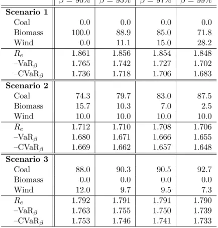
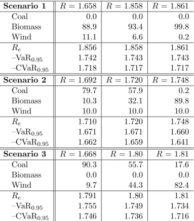
Our approach of combining real options with portfolio optimization could be a useful industry investment device. In fact, the results obtained are very intuitive. Still, the numerical results for the individual technologies are supposed to be rather illustrative. The deeper purpose of this paper is to demonstrate the methodology and the usefulness of the new, theoretical approach, and not to give ad hoc investment advice. More specifically, we examine three CO

price scenarios and we find that there is a trade-off between risk in terms of CVaR and return: Investment does not focus exclusively on the technology with the highest expected return, but diversifies to other technologies in order to keep the associated risk at a minimum.

From the low CO

price scenario going to the high CO

price scenario, there is a shift from a coal-dominated portfolio to a biomass-dominated portfolio.

Furthermore, if we increase β , which is the probability level associated with the CVaR, we observe further diversification away from risky technologies, even if they have comparatively high expected returns. The expected return that we specify to be attained at least, R, is another factor that influences the risk-return trade-off: The higher we set R, the more does the investor tend to increase the share of the technology with the highest expected return at the expense of those that

4Program Package for Emission Reduction Strategies in Energy Use and Supply - Energieversorgungsun- ternehmen; the German term means electric utilities.

5Wind plays a minor role only, since we have constrained it to make up only 10% of the portfolio. Due to its low efficiency, it would space-wise not be feasible to set up larger amounts of wind farms. The data in section 2.2 show that you need 1,389 MW to generate the same amount of electricity as the coal-fired power plant, which is only 500 MW big. For a typical unit size of 1.5 MW per wind mill, this makes already 926 wind mills! It stands to question if such a maximum constraint should also be implemented for biomass. In the UK, for instance, there would not be enough capacities to grow all the biomass, even though the technology as such is quite attractive for the UK. However, biomass is thought to be representative of low emission technologies here, so we do not focus on particular country situations and therefore abstract from this constraint.

have a lower CVaR.

So, we can say that the investment focus shifts from lower risk, CVaR, to higher expected returns, i.e. the investor becomes more return-oriented.

The paper will proceed as follows: First, we will sketch out the real options model, which is an extension of Fuss et al (2006). Section 2 will therefore be subdivided into a descriptive, theoretical part, a part presenting the data used and a part explaining the results for the different technologies and technology chains. Section 3 will give an overview of the CVaR portfolio optimization and will present how we use the CVaR to find optimal portfolios based on the distributions from the real options model. Furthermore, section 3 includes a subsection on the importance of using the CVaR in portfolio optimization in case of non- normal distribution of returns, comparing our approach to the results that one would obtain when using the standard mean-variance portfolio approach. Section 4 concludes.

2 The Real Options Model

2.1 The Framework

The uncertainties that arise in the context of the electricity generator’s investment problem are two-fold. On the one hand, we have uncertainty with respect to output prices. On the other hand, input cost is influenced by fluctuations in the price of CO

emissions.

The cost of capital is taken to be deterministic, which ignores the occurrence of technological uncertainty.

Moreover, capital is not divisible in this model. That means that the investor has the choice to either invest or to leave the investment opportunity open, i.e. it is not possible to install 500 MW at first and then add another 500 MW later etc. Other prices that are not stochastic are fuel prices, even though we do allow for increases of fossil fuel prices over time. Operations and maintenance (O&M) cost and the cost of switching between technologies are deterministic as well. Technological change comes about in the form of decreasing O&M costs and applies only to immature technologies, such as biomass-fired turbines in our experiments.

Electricity prices follow an AR(1) price:

ln P

= c

+ c

ln P

+ ε

, (2.1) where ε

∼ N (0, (σ

)

), with the parameters c

= 1.655, c

= 0.541, and σ

= 0.092 based on spot market data from the European Electricity Exchange (EEX). The CO

prices are modeled based on projections by the MESSAGE model (see Messner and Strubegger (1995) for an overview of the MESSAGE structure). They follow the random walk (RW) with drift.

∆ ln P

= c

+ ε

, (2.2)

6Sometimes the CVaR and variance criteria deliver results that coincide, but this does not necessarily have to be the case as we will see in section 3.5.

7Madlener and Gao (2005) explore the differences in effects when using different policy instruments to support renewable energy. They distinguish between guaranteed feed-in tariffs (such as in Germany) and tradable permits (as suggested by the Kyoto Protocol) and find that subsidies always outperform permits when technological innovation is possible. For our purposes, this distinction between instruments is not that important, which is why we omit it in our analysis.

8Uncertainty of technical change in a real options framework has been analyzed by Farzin et al (1998).

Another application is by Murto (2006).

9Another way of incorporating technological progress has been employed by Kuramboglu et al (2004), who incorporate learning curves for renewable energy into their real options framework. Using data from Turkey, they find that the diffusion of renewable energy technologies will only occur if policies are directed to that cause.

where ∆ ln P

= ln P

− ln P

, ε

∼ N(0, (σ

)

), and parameters c

= 0.056 and σ

= 0.029. The two noise processes are correlated by the factor ρ, which we set equal to 0.7.

Figure 1 below illustrates how these price processes look like.

10 20 30 40 50

20 30 40 50 60 70

Electricity prices

10 20 30 40 50

0 20 40 60 80 100 120 140

CO2 prices

Figure 1: Electricity and CO

Price Paths (These graphs have years on the x-axis and e /MWh and e /t(CO

) on the y-axis respectively.)

The investor thus faces an optimization problem of maximizing discounted expected future returns over all possible future actions under uncertainty about future prices. The problem can be formulated as an optimal control problem with state and control variables. Let x

denote the state that the system is currently in, i.e. it tells you whether the basic plant, the CCS module or both have been built and whether the CCS module is currently running. The starting value of x

is known. Which part of the total plant is currently active is described by the variable m

, where m

is part of the state x

. If no plant is operating, m

= 0; if the basic plant without CCS is operating, m

= 1; and if the plant with additional CCS is operating, m

= 2. Only at t = 0, is m

= 0. Furthermore, let a

be the action, i.e. the control, which the decision-maker chooses to undertake in year t. Possible actions a

include (i) building the basic power plant, (ii) building the power plant including the CCS module, (iii) adding the CCS module, (iv) switching the CCS module off, (v) switching the CCS module on, and (vi) doing nothing. Whether an action is feasible at time t depends on the state at time t. The CCS module can only be switched on, for example, if it has been built already and if it is currently not running. The set of feasible actions at time t is denoted A(x

), and only feasible actions a

∈ A(x

) can be performed. The state in the next period is then determined by the current period’s state x

and the current period’s action a

, formally x

∈ Γ(x

, a

).

As described by Equations (2.1) and (2.2), prices for electricity and CO

follow stochastic processes. The starting values for these processes are known with certainty. The investor can thus solve the optimal control problem of maximizing discounted expected profits,

max

{at}^T_t=0 T

X

t=0

1

(1 + γ)

E [π(x

, a

, P

, P

)], (2.3) subject to a

∈ A(x

) and x

∈ Γ(x

, a

), with x

, P

and P

known and γ the discount rate.

The profit π(·) consists of income from electricity and heat less the cost of fuel, the payments

for CO

emissions, O&M costs and costs associated with the action, c(a

). The production

function is of the Leontieff type, which means that coefficients are fixed. Output is therefore

the product of the rate of efficiency and the amount of the fuel used. Since we assume that all

electricity (and heat), which is generated, can be sold inelastically,

the installed plant will be run continuously, thereby producing a fixed amount of output for a fixed amount of input per year. Any change in investment behavior, therefore, must be due to price uncertainty.

The immediate profit can be calculated as

π(x

, a

, P

, P

) = q

(m

) P

+ q

(m

) P

− q

(m

) P

− q

(m

) P

− OC(m

) − c(a

), (2.4) where P

is the price of heat, P

is the price of the fuel, which will obviously be zero for the renewable energy carriers such as wind, OC is the operational cost per year, q

, q

, q

and q

refer to annual quantities of electricity, heat (where it is important to note that renewable energy carriers do not produce heat as a byproduct of electricity generation), carbon dioxide and fuel, respectively, and m

denotes the type of power plant that is operational at time t (no plant, plant without CCS, plant with CCS). The total discounted income will be divided by total discounted cost, so that we ultimately use returns instead of profits in our CVaR optimization.

It is important to take note of the tradeoffs implied by this profit equation: while the amount of electricity generated will be lower and the operational cost higher if a CCS module is added, the cost arising from carbon payments will be lower as well, since CO

emissions decrease. In order to give the reader a feeling of how significant the difference in carbon emissions is, please consider that in our case the coal-fired power plant without CCS emits 2,155 kt CO

/yr, whereas the one with CCS produces only 292 kt CO

/yr for the same amount of combusted coal (see Table 1). The “clean” power plant thus emits more than seven times less carbon dioxide than the “dirty” power plant. Even though investors will typically install only the dirty power plant in the beginning (because of the significant extra cost in terms of capital when adding the sequestration CCS module), if initial carbon prices are low, they may want to add CCS when carbon prices rise and render instalment of the CCS module more attractive. In our practical application, the focus will therefore be on the timing of installing the CCS module. Since wind mills do not emit carbon dioxide, there is no need for a CCS module and thus there is no technology chain. m

can therefore only assume values 0 (nothing is operational, which only happens in year 0) and 1 (the wind mill is assumed to be operational from year 1 on).

Furthermore, we assume that installing a power plant implies its immediate use and that there is no delay in the realization of the payoffs, that is we abstract from differences in construction times.

As the investor’s problem can be formulated as an optimal control problem and restated in a recursive functional form, we employ dynamic programming

to find the optimal control for the above model. Stochastic dynamic programming is useful when one faces sequential

10This assumption can be justified by acknowledging that distributors will engage into output contracts with generators, specifying amounts of electricity and heat that will be bought off for a prolonged period of time.

11Construction times could be included easily, but we leave them aside for the moment, since this is not our focus and would not change the results qualitatively (if we expand the planning horizon), unless lead times would be dramatically different between different types of plants. Chladn´a et al (2004), who use a similar setup to investigate the pulp and paper sector, also claim that disregarding this aspect has no impact on the interpretation of the simulation results (Chladn´a et al (2004), pages 22-23).

12Dynamic programming was developed in the early fifties by a mathematician called R. Bellman, hence the expression Bellman equation encountered later in this paper.

decision-making, where intermediate stages are not known with certainty. A necessary con- dition for this approach is that the Markov property holds, i.e. that the optimal action for the next period only depends on the current state that the decision-maker is in, and not on past decisions that have brought him/her there. This requirement holds for our problem.

In particular, dynamic programming – stochastic or deterministic – starts from the “back”

of the problem and solves for the optimal decisions recursively.

In our case of electricity capacity planning we will be going through all possible values of the value function depending on all the possible states that the decision-maker can be in depending upon all realizations of prices and thereby determine the optimal action in each stage. In mathematical terms, we formulate the value function corresponding to the maximization problem (2.3), which then has to be maximized by determining the optimal investment strategy {a

}

, where T is the planning horizon. The value function, also called Bellman equation, takes the following form

V (x

, P

, P

) = max

at∈A(xt)

{π(x

, a

, P

, P

) + 1

(1 + γ) E (V (x

, P

, P

)|x

, P

, P

)}, (2.5) where x

∈ Γ(x

, a

) and γ is the discount rate. The value function can be decomposed into the immediate profit, π(x

, a

, P

, P

), which the producer receives upon investment, and the discounted expected continuation value 1/(1 + γ) E (V (x

, P

, P

)|x

, P

, P

). It is important to note that the continuation term is evaluated for the specific state the producer is in, which changes according to the actions he/she undertakes. States which are not feasible will not be considered.

There are different methods of computing the expected value of the value function, E (V (·)). As the type of stochasticity is known, the term can be computed by the means of partial differential equations following the steps in Dixit and Pindyck (1994). The deriva- tions for this approach can be found in Fuss et al (2006), where a similar model is used.

Although the method of using partial differential equations along with appropriate bound- ary conditions is the most elegant way mathematically, this approach has proved – once numerically implemented – to be inflexible to variations and extensions and computationally intensive when using a finer grid.

With respect to the latter problem, the tradeoff between the stability of the numerical scheme and the precision of the final results turns out to be very delicate, which is why we resort to solving the problem at hand with Monte Carlo simulations.

The advantage of the Monte Carlo approach is that it is relatively easy to extend. Also, it has proven to remain efficient in this framework for a rather high degree of complexity and delivers the same results as the partial differential equations approach. In summary therefore, we use backward dynamic programming with forward-moving Monte Carlo simulation.

Of the work reviewed in the introduction, there are various studies that also use Monte Carlo simulation for real options modeling in the electricity sector, e.g. Tseng and Barz (2002),

13This is equivalent to backward optimization procedures that each of us solves more or less subconsciously in everyday situations such as planning a journey to arrive at your destination on time.

14The differential equation needs to be approximated by difference equations which can be solved numeri- cally. This is achieved by constructing a grid, which discretizes the time-price domain. For precise solutions, a fine price grid is necessary that requires smaller time steps to guarantee numerical stability. As a result, the dimension of the problem rises considerably and requires extensive computer resources.

15There is also a third method to move forward and find the optimum decisions. This involves binomial lattice frameworks or binomial decision trees. Even though these are very intuitive and rather flexible when introducing multiple uncertainties and concurrent options, they also tend to get computationally very intensive and therefore not very suitable for our purposes.

who focus on short term generation, and Laurrika and Koljonen (2006), who adopt long term planning horizons.

2.2 The Technologies and the Data

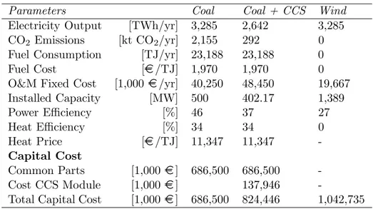
The technologies that we are focussing on in our analysis are coal with the possibility of adding a CCS module, biomass also with the CCS option, and (onshore) wind. These tech- nologies stand representative of fossil fuel technologies (coal), technologies with less emissions (biomass) and zero-emission renewables (wind). We are using data from the International Energy Agency/OECD. The data for biomass have been taken from Leduc et al (forthcom- ing).

They are assembled in Tables 1 and 2 below. Note that electricity output of the three plants (without CCS) is the same, so they are similar in size.

Parameters Coal Coal + CCS Wind

Electricity Output [TWh/yr] 3,285 2,642 3,285 CO

Emissions [kt CO

/yr] 2,155 292 0 Fuel Consumption [TJ/yr] 23,188 23,188 0

Fuel Cost [ e /TJ] 1,970 1,970 0

O&M Fixed Cost [1,000 e /yr] 40,250 48,450 19,667

Installed Capacity [MW] 500 402.17 1,389

Power Efficiency [%] 46 37 27

Heat Efficiency [%] 34 34 0

Heat Price [ e /TJ] 11,347 11,347 -

Capital Cost

Common Parts [1,000 e ] 686,500 686,500 -

Cost CCS Module [1,000 e ] 137,946 -

Total Capital Cost [1,000 e ] 686,500 824,446 1,042,735

Table 1: Power Plant Data for Coal and Wind (Source: “Projected Costs of Generating Electricity 2005 Update”, IEA/OECD, 2005)

In addition, coal prices are assumed to be rising according to the predictions of the same source. We have taken German coal prices, from 2010-2060. The starting prices can be found in Table 1. The biomass fuel prices are from Leduc et al (forthcoming).

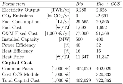
The exorbitantly high O&M costs of the biomass plant is due to the relative immaturity of the technology. With only slight rates of technical change, these costs will drop until they eventually reach about the same magnitude as coal, which is technically very similar in its operation and maintenance. We assume to see such technological progress happen in our model. Another peculiarity of the biomass plant is the negative amount of emissions indicated in the Table. Without the CCS module, biomass already generates zero emissions.

This is not really true, since the biomass plant does generate emissions. However biomass- based electricity production requires the plantation of extra trees or other biomass, which will extract CO

from the atmosphere on top of what is extracted through existing trees and biomass. Therefore, the emissions from biomass-generated electricity are treated as zero, even

16These had to be scaled up to make them comparable with coal, otherwise the output would have been too low.

Parameters Bio Bio + CCS Electricity Output [TWh/yr] 3,285 2,628 CO

Emissions [kt CO

/yr] 0 -2,691 Fuel Consumption [TJ/yr] 29,565 29,565

Fuel Cost [ e /TJ] 1,692 1,692

O&M Fixed Cost [1,000 e /yr] 77,000 91,568

Installed Capacity [MW] 500 400

Power Efficiency [%] 40 32

Heat Efficiency [%] 16 16

Heat Price [ e /TJ] 11,347 11,347

Capital Cost

Common Parts [1,000 e ] 402,029 402,029 Cost CCS Module [1,000 e ] 320,333 Total Capital Cost [1,000 e ] 402,029 722,362

Table 2: Power Plant Data for Biomass (Source: Leduc et al, forthcoming)

though the process will be more complicated in reality: producers would first pay out the CO

charges and receive the subsidies or allowances for their positive CO

externality only later.

That the CO

charges and the subsidies/allowances exactly cancel out is an assumption. With an in-built CCS module, the emissions are reduced, but still the same amount of emissions is subtracted as before, so they will turn negative once everything is accounted for. The discount rate is 4% and the planning horizon is fifty years. All calculations are based on 10,000 simulations.

2.3 Results of the Real Options Model

The real options model is run for three technologies – coal with the possibility to add CCS, biomass with the possibility to add CCS and wind – and for three CO

price scenarios. The scenario where CO

prices show an average yearly price increase

of c

= 5.64% is called the “medium (normal) CO

price scenario” or scenario 2. This is the price process described above. To analyze the impact of CO

prices on investment planning we consider two additional scenarios, one with particularly high CO

prices (scenario 1) and one with particularly low CO

prices (scenario 3). In the first scenario, the average yearly price increase is 1.2c

, i.e. 20% higher than in the normal scenario, in the third scenario the average yearly price increase is 0.5c

, i.e. half the increase of the normal scenario. The variance of the price process is not changed across scenarios, that is σ

= 0.029 in all three scenarios.

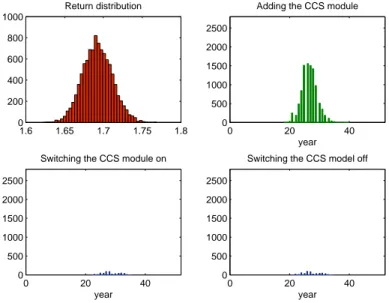
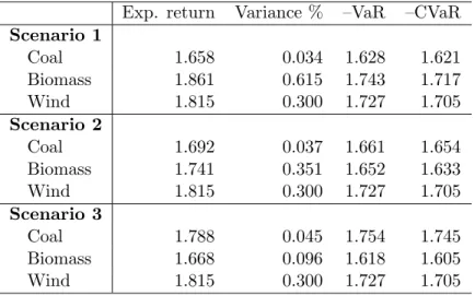
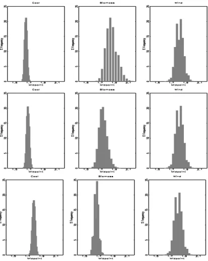
In the following we present numbers and graphs, which are based on the optimal invest- ment strategy for the stochastic control problem stated in (2.3) for a given technology and scenario. As an overall assessment device we calculate the return of investment by taking total discounted income over total discounted cost. Table 3 displays expected return, vari- ance, VaR and CVaR for all three technologies across all three scenarios, Table 4 shows the corresponding correlation matrices. We will present the frequency distribution of the return in the first graph of a panel of four graphs (Figures 2 and 3). The second graph shows the

17To be precise, if we talk about price increases we mean logarithmic price differences.

year, in which the CCS module should be added to the basic power plant. The remaining two graphs show the year, in which it is optimal to switch off the CCS module and in which it is optimal to switch it on again. These graphs actually show frequency distributions of the optimal year when the respective action should be taken. Note that it is never optimal to install the CCS module in the beginning of the planning horizon, since initial CO

prices are too low to trigger such an extra investment immediately. For the third technology, wind power plants, there is no CCS module to add (since there are no CO

emissions) and thus the reader can refer to Figure 4 for the return distribution. Figures 2 and 3 show the graphs described for the coal and biomass technologies in the normal CO

price scenario. The return distributions for all scenarios are displayed in Figure 4 and the corresponding Figures for investment and switching frequencies across all scenarios can be found in Appendix B.

1.6 1.65 1.7 1.75 1.8

0 200 400 600 800 1000

Return distribution

0 20 40

0 500 1000 1500 2000 2500

year Adding the CCS module

0 20 40

0 500 1000 1500 2000 2500

year

Switching the CCS module on

0 20 40

0 500 1000 1500 2000 2500

year

Switching the CCS model off

Figure 2: Return and Investment Frequency Distribution for Coal (Graph 1: The return distribution peaks at 1.69. Graph 2: CCS module is added around year 25 most of the time.

Graphs 3 and 4: Only a slight occurrence of switching the CCS module on and off.)

Figure 2 shows that for the coal technology it is optimal to add the CCS module between year 20 and 35. The return distribution shows a lower expected return than for biomass and wind in the normal CO

price scenario. Figure 4 shows that this gets even worse in the high CO

price scenario. Only in the low CO

price scenario does coal show a higher expected return than biomass, whereas it is still less profitable than wind. This can be verified in Table 3. Furthermore, Table 3 shows that coal is the least risky plant in scenario 3, while it has the most unattractive -CVaR in scenario 1, where CO

prices are high. The probability that the CCS module is switched off after it has been installed is quite low for coal-fired power plants.

So there seems to be relatively low uncertainty about the optimal time when the CCS module

should be added; it is installed as soon as the average CO

price rises above a certain level

(where the variability of the price process seems to be too low to trigger lots of switches). As

can be seen in Figures B.1 and B.3 in Appendix B, the optimal time of adding CCS is clearer

in scenario 1 (there are in fact no off-switches after it has been installed), while in scenario 3

the CO

price is too low to trigger investment in the CCS module most of the time.

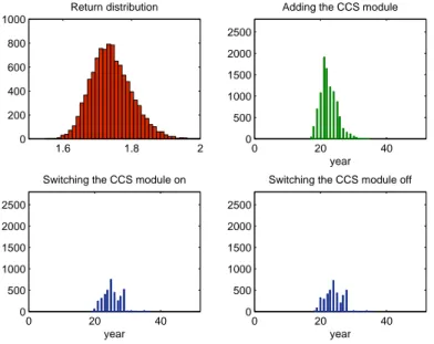
1.6 1.8 2

0 200 400 600 800 1000

Return distribution

0 20 40

0 500 1000 1500 2000 2500

year Adding the CCS module

0 20 40

0 500 1000 1500 2000 2500

year

Switching the CCS module on

0 20 40

0 500 1000 1500 2000 2500

year

Switching the CCS module off

Figure 3: Return and Investment Frequency Distribution for Biomass (Graph 1: The return distribution peaks at 1.72. Graph 2: CCS module is added around year 21 most of the time.

Graphs 3 and 4: Only a slight occurrence of switching the CCS module on and off, but the frequency is higher than for coal.)

Figure 3 shows a slightly different picture for the biomass technology. The CCS module is first built between year 18 and 30 – some years earlier than in the coal technology – and there are significantly more switches before the CCS module is permanently running. The reason for this is that the biomass plant is more heavily influenced by fluctuations in the CO

price than coal due to the comparatively larger reduction in CO

emissions upon CCS installment (and hence larger impact in the cost induced by CO

emissions).

Biomass is the least risky option in scenario 1 in terms of CVaR as can be seen from Table 3.

For wind, the optimization only concerns the date of investment of the plant as such, since the are no “add-ons” as in the case of coal and biomass. Furthermore, the wind plant does not suffer from the volatility of the CO

price, since it does not emit CO

in the first place.

The return distribution displayed in Figure 4 is therefore only based on the simulations of the electricity price. The result of the fact that wind does not have the extra costs imposed by CO

regulations is that the returns for wind are higher than those for coal and biomass.

Also, the expected return, its –CVaR and the variance are the same for all scenarios.

Let us now turn to the statistical properties of the return distributions. As suggested in the introduction, the assumption of normal distributions for the individual risk factors (technologies) makes variance, VaR and CVaR minimization, under some mild technical as- sumptions, equivalent. We will argue, however, that the assumption of joint normality is

18In fact, for biomass this will beincome due to the negative CO2 emissions.

19Note that here the risk analysis would not coincide for the risk measures in terms of CVaR and variance.

Section 3.5 will provide a more detailed analysis of the differences between the mean-variance approach and CVaR as a risk measure.

Exp. return Variance % –VaR –CVaR Scenario 1

Coal 1.658 0.034 1.628 1.621

Biomass 1.861 0.615 1.743 1.717

Wind 1.815 0.300 1.727 1.705

Scenario 2

Coal 1.692 0.037 1.661 1.654

Biomass 1.741 0.351 1.652 1.633

Wind 1.815 0.300 1.727 1.705

Scenario 3

Coal 1.788 0.045 1.754 1.745

Biomass 1.668 0.096 1.618 1.605

Wind 1.815 0.300 1.727 1.705

Table 3: Expected Returns, Variances, CVaR and VaR of the Coal-fired Power Plant, the Biomass-fired Power Plant and Onshore Wind Mills for the Three Scenarios and β=95%

(Scenario 1: high CO

prices; scenario 2: medium CO

prices; scenario 3: low CO

prices.) Coal Biomass Wind

Scenario 1

Coal 1.000 0.305 0.738

Biomass 0.305 1.000 0.836

Wind 0.738 0.836 1.000

Scenario 2

Coal 1.000 0.474 0.783

Biomass 0.474 1.000 0.882

Wind 0.783 0.882 1.000

Scenario 3

Coal 1.000 0.506 0.469

Biomass 0.506 1.000 0.989

Wind 0.469 0.989 1.000

Table 4: Correlation Matrices for the Three Scenarios (Scenario 1: high CO

prices; scenario 2: medium CO

prices; scenario 3: low CO

prices.)

not justified in our application. Note that the assumption of marginal normal distributions does not necessarily guarantee a joint normal distribution. We need to examine all marginal distributions and the joint distribution, where we make use of the so-called copula.

The copula is that part of the joint distribution function, which captures everything describing dependence (after factoring out the marginal distributions). In fact, already a first inspection of the marginal return distributions (see Figure 4) suggests that they are not normal. In considering the copula, we look at the three (bivariate) distribution functions, and thus at

20In fact, marginal normality suffices if one looks at the sum of normally distributed random variables. If one could verify normality for each return distribution, copulas need not be considered. This is not the case here, however; see also Section 3.5.

the three copulas, describing coal/biomass, coal/wind and biomass/wind dependence.

Formally, let F be an two-dimensional distribution function of random variables X and Y with marginal distribution functions F

and F

. Then,

F (x, y) = C(F

(x), F

(y)),

where, under some technical conditions, C is unique. For more details refer to Appendix C. One specific copula, which is implicitly used all the time, is the normal copula; this is the copula implied by the joint normal distribution. One property of the normal copula is that it displays symmetric dependence, that is, dependence in the lower and upper tail of the distribution is the same. One way of testing normality, or more precisely, symmetric dependence, is to consider a copula which allows for potentially different lower and upper tail dependence and to check whether the restriction of equal lower and upper tail dependence can be rejected. Loosely speaking, lower tail dependence λ

describes how two random variables move together in the lower tail of the distribution. Upper tail dependence λ

describes how two random variables move together in the upper tail of the distribution. A higher λ

(λ

) obviously means a higher degree of dependence in the lower (upper) tail. For a more formal definition see Appendix C. If our test showed that the dependence between individual returns is not symmetric, the implied joint distribution could not be the normal one. And hence the variance, VaR and CVaR minimization would not necessarily yield the same results.

In order to conduct such a test we need to consider a fairly flexible copula allowing for different lower and upper tail dependence. The Clayton and the Gumbel copula, two widely used one-parametric Archimedean copulas, are too restrictive in the sense that they allow of only lower (Clayton) or only upper (Gumbel) positive tail dependence, while the other tail dependence is always zero. This – necessarily asymmetric – type of copula is not suitable for our application and thus we decided to use the two-parametric BB1 copula. The BB1 copula allows for asymmetric and symmetric dependence and it nests the popular Clayton and the Gumbel copulas. Its parametric form is

C(u, v) = {1 + [(u

− 1)

+ (v

− 1)

]

}

,

where θ > 0 and δ ≥ 1. Details can be found in Appendix C. We estimate the BB1 copula through maximum likelihood, where we take empirical distributions for the marginal returns.

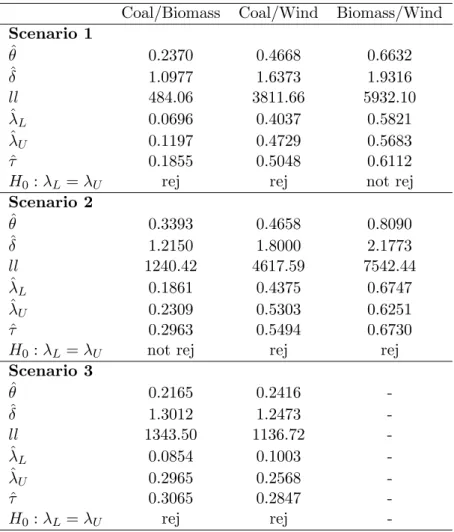
Then we restrict this same copula in the sense that lower tail dependence equals upper tail dependence and conduct a likelihood ratio test. In nearly all cases the null hypothesis of equal lower and upper tail dependence (H

: λ

= λ

) can be rejected at the 5% significance level. Table 5 shows the results for all technologies in the three different scenarios. In all cases (except two) the assumption of symmetric dependence can be rejected; in these cases, the assumption of joint normality would not be appropriate.

Interestingly, for biomass/wind a larger degree of dependence is prevalent in the lower tail of the distribution (in all scenarios); the difference between the lower and upper tail dependence is small, however. On the other hand a larger degree of dependence seems to be present in the upper part tail of the distribution for coal/wind and coal/biomass (in all scenarios). Interpreting these results is not straightforward, since the underlying model is complex and generally includes two stochastic processes, the electricity and the CO

price process. Assuming that, ceteris paribus, higher returns are triggered by higher income through

21Note that the dependence between biomass and wind in scenario 3 is too large to estimate the copula parameters. The linear correlation is 0.99, as can be seen from Table 4.

Coal/Biomass Coal/Wind Biomass/Wind Scenario 1

θ ˆ 0.2370 0.4668 0.6632

δ ˆ 1.0977 1.6373 1.9316

ll 484.06 3811.66 5932.10

λ ˆ

0.0696 0.4037 0.5821

λ ˆ

0.1197 0.4729 0.5683

ˆ

τ 0.1855 0.5048 0.6112

H

: λ

= λ

rej rej not rej

Scenario 2

θ ˆ 0.3393 0.4658 0.8090

δ ˆ 1.2150 1.8000 2.1773

ll 1240.42 4617.59 7542.44

λ ˆ

0.1861 0.4375 0.6747

λ ˆ

0.2309 0.5303 0.6251

ˆ

τ 0.2963 0.5494 0.6730

H

: λ

= λ

not rej rej rej

Scenario 3

θ ˆ 0.2165 0.2416 -

δ ˆ 1.3012 1.2473 -

ll 1343.50 1136.72 -

λ ˆ

0.0854 0.1003 -

λ ˆ

0.2965 0.2568 -

ˆ

τ 0.3065 0.2847 -

H

: λ

= λ

rej rej -

Table 5: Copula Results for Return Distributions (The bivariate BB1 copula with parameters θ and δ is estimated. We report parameter estimates, the log-likelihood (ll), and implied lower (λ

) and upper (λ

) tail dependence and Kendall’s rank correlation tau (τ ). We additionally provide the results of a likelihood ratio test, where the restricted copula is the symmetric BB1 in the sense that lower tail dependence is equal to upper tail dependence.)

higher electricity prices, the results indicate that for coal/wind and coal/biomass the observed dependence is higher in increasing electricity markets, while for biomass/wind it is higher in decreasing electricity markets. The term “increasing markets” means that prices in these markets increase; the same applies to decreasing markets. To be able to provide a more subtle picture of the impact of the two sources of uncertainty (electricity and CO

prices), a more detailed analysis is required.

3 CVaR-based Portfolio Optimization

3.1 CVaR as a Risk Measure

Making an investment decision involves taking a certain admissible level of risk. Usually a

criterion to discern the risk related to different investment strategies – a specific risk measure

Figure 4: Return Distributions of Coal, Biomass and Wind Technologies (The top row shows returns for high CO

prices, the middle row shows returns for medium CO

prices, the bottom row shows returns for low CO

prices. The number of simulations is 10

.)

– is needed to select an appropriate investment strategy. We suggest using CVaR as the risk measure in our investment model in the electricity sector. Here is a short discussion regarding the suggested approach.

Value-at-Risk (VaR) is a widely used measure of risk and it is part of the Basel II method- ology of the international standards for measuring the adequacy of a bank’s capital, as stated in the introduction. However, VaR has several disadvantages, as for example discussed in the papers by Rockafellar and Uryasev (2000) and Palmquist et al (2002). The issue of coherency of risk measures and VaR is debated in the papers by Arztner et al (1997) and Rockafellar and Uryasev (2002). Contributions dealing with CVaR applications have also grown rapidly within the past few years. CVaR is becoming increasingly popular in various areas of risk management including energy risk management (Doege et al, 2006), crop insurance (Schnitkey et al, 2004 and Liu et al, 2006), power portfolio optimization (Unger and L¨ uthi, 2002), hedge funds applications (Krokhmal et al, 2003), pension funds management (Bogentoft et al, 2001), and multi-currency asset allocations (Topaloglou et al, 2002).

CVaR offers a number of improvements over VaR; first it may be considered as an extension

of this commonly used risk measure. CVaR provides a sort of approximation of VaR in the sense that it is an upper bound of VaR. Hence minimizing CVaR instead of VaR in portfolio optimization may be considered a more “conservative” approach. Another advantage of using CVaR as a risk measure is that CVaR provides the decision maker with more information than VaR. The latter indicates the maximum value of losses, which an investor incurs given some pre-defined probability (most probable event); it does not reveal anything about how big the losses could be in case the less probable event occurs, while CVaR does. CVaR thus provides the investor with valuable information about which losses he/she should expect in the “low probability” case. From this point of view, CVaR offers potential advantages to hedge investments into funds or industry sectors regulated by VaR restrictions on their assets risk. An important property of CVaR which matters in applications is that CVaR is relatively easy to calculate. Basically, the calculation of CVaR can be reduced to a linear programming problem which may effectively be solved using a broad range of applied software available on the market.

We will define CVaR according to the paper by Rockafellar and Uryasev (2000). Let f(x, y) be the loss function depending on the investment strategy x ∈ R

and the random vector y ∈ R

. The probability of f(x, y) not exceeding some fixed threshold level α is

Ψ(x, α) = Z

f(x,y)≤α

p(y)dy.

The β-VaR is defined by the following equation

VaR

(x) = α

(x) = min { α | Ψ(x, α) ≥ β },

which means that with probability β the losses will not exceed the threshold level α

(x) for a given investment strategy x.

The β -CVaR is finally defined by

CVaR

(x) = φ

(x) = (1 − β)

Z

f(x,y)≥αβ(x)

f(x, y)p(y)dy,

which is the expected loss given that the loss exceeds the VaR level, hence conditional expected loss, or Conditional Value-at-Risk. (Note that when clear from the context we will drop β and/or x).

An important parameter of a risk estimation procedure is the confidence level β, which describes the probability of the event, when our losses exceed a specific (known) level. The risk measure depends on this confidence level β , so to each β corresponds some particular CVaR risk measure, that is we can more precisely talk about β-CVaR.

3.2 Portfolio Optimization: Minimizing Risk

We assume that we have n different technology chains (i.e. coal plus CCS as the first “chain”,

biomass plus CCS as the second one and wind as a single technology) at our disposal to

invest. Values y

, i = 1, . . . , n reflect the return of investment (ROI) for each technology

chain. We assume the vector y = [y

, . . . , y

]

∈ R

of ROIs to be a random vector having

some distribution. We describe the investment strategy using the vector x = [x

, . . . , x

]

∈

R

where the scalar value x

, i = 1, . . . , n reflects the portion of capital invested into the