The Burrows-Wheeler Transform:
Theory and Practice
Giovanni Manzini 1,2
1
Dipartimento di Scienze e Tecnologie Avanzate, Universit` a del Piemonte Orientale
“Amedeo Avogadro”, I-15100 Alessandria, Italy.
2
Istituto di Matematica Computazionale, CNR, I-56126 Pisa, Italy.
Abstract. In this paper we describe the Burrows-Wheeler Transform (BWT) a completely new approach to data compression which is the basis of some of the best compressors available today. Although it is easy to intuitively understand why the BWT helps compression, the analysis of BWT-based algorithms requires a careful study of every single algorithmic component. We describe two algorithms which use the BWT and we show that their compression ratio can be bounded in terms of the k-th order empirical entropy of the input string for any k ≥ 0. Intuitively, this means that these algorithms are able to make use of all the regularity which is in the input string.
We also discuss some of the algorithmic issues which arise in the com- putation of the BWT, and we describe two variants of the BWT which promise interesting developments.
1 Introduction
It seems that there is no limit to the amount of data we need to store in our computers, or send to our friends and colleagues. Although the technology is providing us with larger disks and faster communication networks, the need of faster and more efficient data compression algorithms seems to be always increasing. Fortunately, data compression algorithms have continued to evolve in a continuous progress which should not be taken for granted since there are well known theoretical limits to how much we can squeeze our data (see [31] for a complete review of the state of the art in all fields of data compression).
Progress in data compression usually consists of a long series of small im- provements and fine tuning of algorithms. However, the field experiences occa- sional giant leaps when new ideas or techniques emerge. In the field of lossless compression we have just witnessed to one of these leaps with the introduction of the Burrows-Wheeler Transform [7] (BWT from now on). Loosely speaking, the BWT produces a permutation bw(s) of the input string s such that from bw(s) we can retrieve s but at the same time bw(s) is much easier to compress.
The whole idea of a transformation that makes a string easier to compress is
completely new, even if, after the appearance of the BWT some researchers rec-
ognized that it is related to some well known compression techniques (see for
example [8, 13, 18]).
The BWT is a very powerful tool and even the simplest algorithms which use it have surprisingly good performances (the reader may look at the very simple and clean BWT-based algorithm described in [26] which outperforms, in terms of compression ratio, the commercial package pkzip). More advanced BWT-based compressors, such as bzip2 [34] and szip [33], are among the best compressors currently available. As can be seen from the results reported in [2]
BWT-based compressors achieve a very good compression ratio using relatively small resources (time and space). Considering that BWT-based compressors are still in their infancy, we believe that in the next future they are likely to become the new standard in lossless data compression.
In this paper we describe the BWT and we explain why it helps compression.
Then, we describe two simple BWT-based compressors and we show that their compression ratio can be bounded in terms of the empirical entropy of the input string. We briefly discuss the algorithms which are currently used for computing the BWT, and we conclude describing two recently proposed BWT variants.
2 Description of the BWT
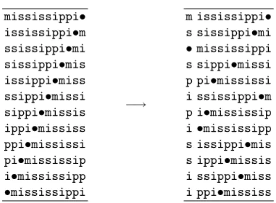
The Burrows-Wheeler transform [7] consists of a reversible transformation of the input string s. The transformed string, that we denote by bw(s), is simply a permutation of the input but it is usually much easier to compress in a sense we will make clear later. The transformed string bw(s) is obtained as follows 1 (see Fig. 1). First we add to s a unique end-of-file symbol •. Then we form a (conceptual) matrix containing all cyclic shifts of s•. Then, we sort the rows of this matrix in right-to-left lexicographic order (considering • to be the symbol with the lowest rank) and we set bw(s) to be the first column of the sorted matrix with the end-of-file symbol removed. Note that this process is equivalent to the sorting of s using, as a sort key for each symbol, its context, that is, the set of symbols preceding it. The output of the Burrows-Wheeler transform is the string bw(s) and the index I in the sorted matrix of the row starting with the end-of-file symbol 2 (for example, in Fig. 1 we have I = 3).
Although it may seem surprising, from bw(s) and I we can always retrieve s.
We show how this can be done for the example in Fig. 1. By inserting the symbol • in the Ith position of bw(s) we get the first column F of the sorted cyclic shifts matrix. Since every column of the matrix is a permutation of s•, by sorting the symbols of F we get the last column L of the sorted matrix.
Let s i (resp. F i , L i ) denote the i-th symbol of s (resp. F, L). The fundamental observation is that for i = 2, . . . , |s| + 1, F i is the symbol which follows L i inside s. This property enables us to retrieve the string s symbol by symbol. Since we sort the cyclic shifts matrix considering • to be the symbol with the lowest
1
To better follow the example the reader should think s as a long string with a strong structure (e.g., a Shakespeare play). Data compression is not about random strings!
2
In the original formulation rows are sorted in left-to-right lexicographic order and
there is no end-of-file symbol. We use this slightly modified definition since we find
it easier to understand.
mississippi•
ississippi•m ssissippi•mi sissippi•mis issippi•miss ssippi•missi sippi•missis ippi•mississ ppi•mississi pi•mississip i•mississipp
•mississippi
−→
m ississippi•
s sissippi•mi
• mississippi s sippi•missi p pi•mississi i ssissippi•m p i•mississip i •mississipp s issippi•mis s ippi•missis i ssippi•miss i ppi•mississ
Fig. 1. Example of Burrows-Wheleer transform. We have bw(mississippi) = msspipissii. The matrix on the right is obtained sorting the rows in right-to-left lexi- cographic order.
rank, it follows that F 1 is the first symbol of s. Thus, in our example we have s 1 = m. To get s 2 we notice that m appears in L only in position 6, thus from our previous observation we get s 2 = F 6 = i. Now we try to retrieve s 3 and we have a problem since i appears in L four times, in the positions L 2 , . . . , L 5 . Hence, F 2 , . . . , F 5 are all possible candidates for s 3 . Which is the right one?
The answer follows observing that the order in which the four i’s appear in F coincides with order in which they appear in L since in both cases the order is determined by their context (the set of symbols immediately preceding each i).
This is evident by looking at sorted matrix in Fig. 1. The order of the four i’s in L is determined by the (right-to-left) lexicographic order of their contexts (which are m, mississipp, miss, mississ). The same contexts determine the order of the four i’s in F . When we are back-transforming s we do not have the complete matrix and we do not know these contexts, but the information on the relative order still enable us to retrieve s. Continuing our example, we have that since s 2 = F 6 is the first i in F we must look at the first i in L which is L 2 . Hence, s 3 = F 2 = s. Since s 3 is the first s in F , it corresponds to L 9 and s 4 = F 9 = s.
Since F 9 is the third s in F it corresponds to L 11 and we get s 5 = F 11 = i. The process continues until we reach the end-of-file symbol.
Why should we care about the permuted string bw(s)? The reason is that the string bw(s) has the following remarkable property: for each substring w of s, the symbols following w in s are grouped together inside bw(s). This is a consequence of the fact that all rotations ending in w are consecutive in the sorted matrix.
Since, after a (sufficiently large 3 ) context w only a few symbols are likely to be seen, the string bw(s) will be locally homogeneous, that is, it will consist of the concatenation of several substrings containing only a few distinct symbols.
3
How large depends on the structure on the input. However (and this is a fundamental
feature of the Burrows-Wheeler transform) our argument holds for any context w.
To take advantage of this particular structure, Burrows and Wheeler sug- gested to process bw(s) using Move-to-Front recoding [6, 27]. In Move-to-Front recoding the symbol α i is coded with an integer equal to the number of distinct symbols encountered since the previous occurrence of α i . In other words, the encoder maintains a list of the symbols ordered by recency of occurrence (this will be denoted the mtf list). When the next symbol arrives, the encoder outputs its current position in the mtf list and moves it to the front of the list. There- fore, a string over the alphabet A = {α 1 , . . . , α h } is transformed to a string over {0, . . . , h − 1} (note that the length of the string does not change) 4 .
So far we still have a string ˆ s = mtf(bw(s)) which has exactly the same length as the input string. However, the string ˆ s will be in general highly compressible.
As we have already noted, bw(s) consists of several substrings containing only a few distinct symbols. As a consequence, the Move-to-Front encoding of each of these substrings will generate many small integers. Therefore, although the string ˆ
s = mtf(bw(s)) contains enough information to retrieve s, it mainly consists of 0’s, 1’s, and other small integers. For example, if s is an English text ˆ s usually contains more than 50% 0’s. The actual compression is performed in the final step of the algorithm which exploits this “skeweness” of ˆ s. This is done using for example a simple zeroth order algorithm such as Huffman coding [36] or arithmetic coding [38]. These algorithms are designed to achieve a compression ratio equal to the zeroth order entropy of the input string s which is defined by 5
H 0 (s) = −
h
X
i=1
n i
n log n i n
, (1)
where n = |s| and n i is the number of occurrences of the symbol α i in s. Ob- viously, if ˆ s consists mainly of 0’s and other small integers H 0 (ˆ s) will be small and ˆ s will be efficiently compressed by a zeroth order algorithm.
Note that neither Huffman coding nor arithmetic coding are able to achieve compression ratio H 0 (s) for every string s. However, arithmetic coding can get quite close to that: in [15] Howard and Vitter proved that the arithmetic coding procedure described in [38] is such that for every string s its output size Arit(s) is bounded by
Arit(s) ≤ |s|H 0 (s) + µ 1 |s| + µ 2 (2) with µ 1 ≈ 10 −2 . In other words, the compression ratio Arit(s)/|s| is bounded by the entropy plus a small constant plus a term which vanishes as |s| → ∞.
In the following we denote with BW0 the algorithm bw + mtf + Arit, that is, the algorithm which given s returns Arit(mtf(bw(s))). BW0 is the basic algorithm described in [7] and it has been tested in [13] (under the name bs-Order0). Al- though it is one of the simplest BWT-based algorithms, it has better performance than gzip which is the current standard for lossless compression.
4
Obviously, to completely determine the encoding we must specify the status of the mtf list at the beginning of the procedure.
5
In the following all logarithms are taken to the base 2, and we assume 0 log 0 = 0.
Note that the other BWT-based compressors described in the literature do not differ substantially from BW0. Most of the differences are in the last step of the procedure, that is, in the techniques used for exploiting the skeweness of
˜
s = mtf(bw(s)). A technique commonly used by BWT compressors is run-length encoding which we will discuss in the next section. Move-to-Front encoding is used by all BWT compressors with the only exceptions of [4] and [33] which use slightly different encoding procedures.
3 BWT compression vs entropy
It is generally known that the entropy of a string constitutes a lower bound to how much we can compress it. However, this statement is not precise since there are several definitions of entropy, each one appropriate for a particular model of the input. For example, in the information theoretic setting, it is often assumed that the input string is generated by a finite memory ergodic source S, sometimes with additional properties. A typical result in this setting is that the average compression ratio 6 achieved by a certain algorithm approaches the entropy of the source as the length of the input goes to infinity. This approach has been very successful in the study of dictionary based compressors such as lz77, lz78 and their variants (which include gzip, pkzip, and compress).
Compression algorithms can be studied also in a worst-case setting which is more familiar to people in the computer science community. In this setting the compression ratio of an algorithm is compared to the empirical entropy of the input. The empirical entropy, which is a generalization of (1), is defined in terms of the number of occurrences of each symbol or group of symbols in the input. Since it is defined for any string without any probabilistic assumption, the empirical entropy naturally leads to establish worst case results (that is, results which hold for every possible input string).
The first results on the compression of BWT-based algorithms have been proved in the information theoretic setting. In [28, 29] Sadakane has proposed and analyzed three different algorithms based on the BWT. Assuming the input string is generated by a finite-order Markov source, he proved that the average compression ratio of these algorithms approaches the entropy of the source. More recently, Effros [10] has considered similar algorithms and has given bounds on the speed at which the average compression ratio approaches the entropy. Al- though these results provide useful insight on the BWT, they are not completely satisfying. The reason is that these results deal with algorithms which are not realistic (and in fact are not used in practice). For example, some of these algo- rithms require the knowledge of quantities which are usually unknown such as the order of the Markov source or the number of states in the ergodic source.
In the following we consider the algorithm BW0 = bw + mtf + Arit described in the previous section and we show that for any string s the output size BW0(s) can be bounded in terms of the empirical entropy of s. To our knowledge, this is
6
The average is computed using the probability of each string of being generated by
the source S .
the first analysis of a BWT-based algorithm which does not rely on probabilistic assumptions. The details of the analysis can be found in [21].
Let s be a string of length n over the alphabet A = {α 1 , . . . , α h }, and let n i denote the number of occurrences of the symbol α i inside s. The zeroth order empirical entropy of the string s is defined by (1). The value |s|H 0 (s), represents the output size of an ideal compressor which uses − log n n
ibits for coding the symbol α i . It is well known that this is the maximum compression we can achieve using a uniquely decodable code in which a fixed codeword is assigned to each alphabet symbol. We can achieve a greater compression if the codeword we use for each symbol depends on the k symbols preceding it. For any length-k word w ∈ A k let w s denote the string consisting of the characters following w inside s. Note that the length of w s is equal to the number of occurrences of w in s, or to that number minus one if w is a suffix of s. The value
H k (s) = 1
|s|
X
w∈A
k|w s |H 0 (w s ) (3)
is called the k-th order empirical entropy of the string s. The value |s|H k (s) represents a lower bound to the compression we can achieve using codes which depend on the k most recently seen symbols. Not surprisingly, for any string s and k ≥ 0, we have H k+1 (s) ≤ H k (s).
Example 1. Let s = mississippi. From (1) we get H 0 (s) ≈ 1.823. For k = 1 we have m s = i, i s = ssp, s s = sisi, p s = pi. By (1) we have H 0 (i) = 0, H 0 (ssp) = 0.918, H 0 (sisi) = 1, H 0 (pi) = 1. According to (3) the first order
empirical entropy is H 1 (s) ≈ 0.796. u t
We now show that the compression achieved by BW0 can be bounded in terms of the empirical k-th order entropy of the input string for any k ≥ 0. From (3) we see that to achieve the k-th order entropy “it suffices”, for any w ∈ A k , to compress the string w s up to its zeroth order entropy H 0 (w s ). One of the reasons for which this is not an easy task is that the symbols of w s are scattered within the input string. But this problem is solved by the Burrows-Wheeler transform! In fact, from the discussion of the previous section we know that for any w the symbols of w s are grouped together inside bw(s). More precisely, bw(s) contains as a substring a permutation of w s . Permuting the symbols of a string does not change its zeroth order entropy. Hence, thanks to the Burrows- Wheeler transform, the problem of achieving H k (s), is reduced to the problem of compressing several portions of bw(s) up to their zeroth order entropy. Note that even this latter problem is not an easy one. For example, compressing bw(s) up to its zeroth order entropy is not enough as the following example shows.
Example 2. Let s 1 = a n b, s 2 = b n a. We have |s 1 |H 0 (s 1 ) + |s 2 |H 0 (s 2 ) ≈ 2 log n.
If we compress the concatenation s 1 s 2 up to its zero order entropy, we get an
output size of roughly |s 1 s 2 |H 0 (s 1 s 2 ) = 2n + 1 bits. u t
The key element for achieving the k-th order entropy is mtf encoding. We have
seen in the previous section that processing bw(s) with mtf produces a string
which is in general highly compressible. In [21] it is shown that this intuitive notion can be transformed to the following quantitative result.
Theorem 1. Let s be any string over the alphabet {α 1 , . . . , α h }, and s ˜ = mtf(s).
For any partition s = s 1 · · · s t we have
|˜ s|H 0 (˜ s) ≤ 8 t
X
i=1
|s i |H 0 (s i )
+ 2
25 |s| + t(2h log h + 9). (4) u t The above theorem states that the entropy of mtf(s) can be bounded in terms of the weighted sum
|s 1 |
|s| H 0 (s 1 ) + |s 2 |
|s| H 0 (s 2 ) + · · · + |s t |
|s| H 0 (s t ) (5)
for any partition s 1 s 2 · · · s t of the string s. We do no claim that the bound in (4) is tight (in fact, we believe it is not). In most cases the entropy of mtf(s) turns out to be much closer to the sum (5). For example, for the strings in Example 2 we have mtf(s 1 s 2 ) = 0 n 10 n 1 so that H 0 (mtf(s 1 s 2 )) is exactly equal to |s |s|
1| H 0 (s 1 ) + |s |s|
2| H 0 (s 2 ).
From (4) it follows that if we compress mtf(s) up to its zeroth order entropy the output size can be bounded in terms of the sum P
i |s i |H 0 (s i ). This result enables us to prove the following bound for the output size of BW0.
Corollary 1. For any string s over A = {α 1 , . . . , α h } and k ≥ 0 we have BW0(s) ≤ 8|s|H k (s) +
µ 1 + 2 25
|s| + h k (2h log h + 9) + µ 2 , (6) where µ 1 , µ 2 are defined in (2).
Proof. From the above discussion we know that bw(s) can be partitioned into at most h k substrings each one corresponding to a permutation of a string w s with w ∈ A k . Hence, by (3) and Theorem 1 the string ˜ s = mtf(bw(s)) is such that
|˜ s|H 0 (˜ s) ≤ 8|s|H k (s) + 2
25 |s| + h k (2h log h + 9). (7) In addition, by (2) we know that
BW0(s) = Arit(˜ s) ≤ |˜ s|H 0 (˜ s) + µ 1 |˜ s| + µ 2 ,
which, combined with (7), proves the corollary. u t
Note that any improvement in the bound (4) yields automatically to an
improvement in the bound of Corollary 1. Although the constants in (6) are
admittedly too high for our result to have a practical impact, it is reassuring
to know that an algorithm which works well in practice has nice theoretical
properties. Our result somewhat guarantee that BW0 remains competitive for very long strings, or strings with very small entropy. From this point of view, the most “disturbing” term in (6) is (µ 1 + 2/25) |s| which represents a constant overhead per input symbol. This overhead comes in part (the term µ 1 ) from the bound (2) on arithmetic coding, and in part (the term 2/25) from Theorem 1 on mtf encoding. However, in our opinion, the inefficiency which results from Corollary 1 is also due to the fact that the bound provided by the k-th order entropy is sometimes too conservative and cannot be reasonably achieved. This is shown by the following example.
Example 3. Let s = cc(ab) n . We have a s = b n , b s = a n−1 , c s = ca. This yields
|s|H 1 (s) = nH 0 (b n ) + (n − 1)H 0 (a n−1 ) + 2H 0 (ca) = 2.
Hence, to compress s (which has length 2n + 2) up to its first order entropy we
should be able to encode it using only 2 bits. u t
The reason for which in the above example |s|H 1 (s) fails to provide a reasonable bound, is that for any string consisting of multiple copies of the same symbol, for example s = a n , we have H 0 (s) = 0. Since the output of any compression algorithm must contain enough information to recover the length of the input, it is natural to consider the following alternative definition of zeroth order empirical entropy. For any string s let
H 0 ∗ (s) =
0 if |s| = 0,
(1 + blog |s|c)/|s| if |s| 6= 0 and H 0 (s) = 0,
H 0 (s) otherwise.
(8)
Note that 1+blog |s|c is the number of bits required to express |s| in binary. In [21]
it is shown that starting from H 0 ∗ one can define a k-th order modified empirical entropy H k ∗ which provides a more realistic lower bound to the compression ratio we can achieve using contexts of size k or less.
The entropy H k ∗ has been used to analyze a variant of the algorithm BW0.
This variant, called BW0 RL , has an additional step consisting in the run-length encoding of the runs of zeroes produced by the Move-to-Front transformation 7 . As reported in [12] many BWT-based compressors make use of this technique.
In [21] it is shown that for any k ≥ 0 there exists a constant g k such that for any string s
BW0 RL (s) ≤ (5 + )|s|H k ∗ (s) + g k , (9) where BW0 RL (s) is the output size of BW0 RL , ≈ 10 −2 , and H k ∗ (s) is the modified k-order empirical entropy. The significance of (9) is that the use of run-length encoding makes it possible to get rid of the constant overhead per input symbol, and to reduce the size of the multiplicative constant associated to the entropy.
7
This means that every sequence of m zeros produced by mtf encoding is replaced by
the number m written in binary.
To our knowledge, a bound similar to (9) has not been proven for any other compression algorithm. Indeed, for many of the better known algorithms (in- cluding some BWT-based compressors) one can prove that a similar bound can- not hold. For example, although the output of lz77 and lz78 is bounded by
|s|H k (s) + O(|s| log |s|/ log log |s|), for any λ > 0 we can find a string s such that the output of these algorithms is greater than λ|s|H 1 ∗ (s) (see [16], obviously for such strings we have H k (s) log |s|/ log log |s|). The algorithm PPMC [25], which has been the state of the art compressor for several years, predicts the next symbol on the basis of the l previous symbols, where l is a parameter of the algorithm. Thus, there is no hope that its compression ratio approaches the k-th order entropy for k > l. Two algorithms for which a bound similar to (9) might hold for any k ≥ 0 are DMC [9] and PPM* [8]. Both of them predict the next symbol on the basis of a (potentially) unbounded context and they work very well in practice. Unfortunately, these two algorithms have not been analyzed theoretically, and an analysis does not seem to be around the corner.
4 Algorithmic issues
In this section we discuss some of the algorithmic issues which arise in the realization of an efficient compressor based on the BWT. Our discussion is by no means exhaustive; many additional useful information can be found for example in [3] and [12]. The reader who wants to know everything about an efficient BWT- based compressor may look at the source code of the algorithm bzip2 which is freely available [34].
Most BWT-based compressors process the input file in blocks. A single block is read, compressed and written to the output file before the next one is con- sidered. This technique provides a simple means for controlling the memory requirements of the algorithm and a limited capability of error recovering. As a general rule, the larger is the block size the slower is the algorithm and the better is the compression. In bzip2 the block size can be chosen by the user in the range from 100Kb to 900Kb.
The most time consuming step of BWT-based algorithms is the computation of the transformed string bw(s). In Sect. 2 we defined bw(s) to be the string obtained by lexicographic sorting the prefixes of s. This view has been adopted in some implementations, whereas in other cases bw(s) is defined considering the lexicographic sorting of the suffixes of s. This difference does not affect signifi- cantly neither the running time nor the final compression. From an algorithmic point of view the problems of sorting suffixes or prefixes are equivalent; in the following we refer to the suffix sorting problem which is more often encountered in the algorithmic literature.
The problem of sorting all suffixes of a string s has been studied even be- fore the introduction of the BWT because of its relevance in the field of string matching. The problem can be solved in linear time (that is, proportional to
|s|), by building a suffix tree for s and traversing the leaves from left to right.
There are three “classical” linear time algorithms for the construction of a suffix
tree [23, 35, 37]. These algorithms require linear space, unfortunately with large multiplicative constants. The most space economical algorithm is the one by McCreight [23] which, for a string of length n, requires 28n bytes 8 in the worst case. For BWT algorithms this large storage requirement is a serious drawback since it limits the block size that can be used in practice (as we mentioned be- fore, larger blocks usually yield better compression). For this reason suffix tree algorithms have not been commonly used for computing the BWT. Recently this state of affair has begun to change. A currently active area of research is the development of compact representations of suffix trees [1, 17]. For example, one the algorithms in [17] builds a suffix tree using 20 bytes per input symbol in the worst case and 10 bytes per input symbol on average for “real life” files. The use of these space economical suffix tree construction algorithms for the BWT has been discussed in [4].
A data structure which is commonly used as an alternative to the suffix tree is the suffix array [20]. The suffix array A of a string s is such that A i contains the index of the starting point of the ith suffix in the lexicographic order. For example for s = mississippi the suffix array is A = [11, 8, 5, 2, 1, 10, 9, 7, 4, 6, 3].
Obviously, from the suffix array one can immediately derive the string bw(s). The suffix array for a string of length n can be computed in O(n log n) time using the algorithms by Manber and Myers [20] or Larsson and Sadakane [19]. The major advantage of suffix array algorithms with respect to suffix tree algorithms is their small memory requirements. Both Manber-Myers’s and Larsson-Sadakane’s algorithms only need an auxiliary array of size n in addition to the space for their input and output (the string s and the suffix array A). Their total space requirement is therefore 9 bytes for input symbol.
In [19] Larsson and Sadakane report the results of a thorough comparison between several suffix sorting algorithms. They use test files of size up to 125MB therefore they only consider algorithms with small memory requirements. In ad- dition to their suffix array construction algorithm they have tested a space eco- nomical suffix tree construction algorithm described in [17], the Manber-Myers suffix array construction algorithm as implemented in [24], and the Bentley- Sedgewick string sorting algorithm [5]. From the results of their extensive testing it turns out that the performances of suffix sorting algorithms are significantly influenced by the average Longest Common Prefix (average lcp from now) be- tween adjacent suffixes in the sorted order 9 . For files with a small average lcp (up to 20.1), the fastest algorithm is the Bentley-Sedgewick algorithm. Note that this is a generic string sorting algorithm which do not make explicit use of the fact that the strings to be sorted are the suffixes of a given string. For files with a larger average lcp the fastest algorithm is Larsson-Sadakane’s. For the file pic
— consisting of a black and white bitmap with an average lcp of 2,353.4 —
8
In this section space requirements are computed assuming that an input symbol requires 1 byte and an integer requires 4 bytes.
9
The average lcp can be seen also as the average number of symbols which must be
inspected to distinguish between two adjacent suffixes in the sorted order.
the fastest algorithm is the space-economical suffix tree construction algorithm from [17].
5 BWT variants
In this section we describe two recently proposed variants of the Burrows Wheeler transform which we believe promise interesting developments.
The first variant is due to Schindler [32] and consists of a transform bws k
which is faster than the BWT and produces a string which is still highly com- pressible in the sense discussed in Section 2. Given a parameter k > 0, Schindler’s idea is to sort the rows of the cyclic shifts matrix of Fig. 1 according to their last k symbols only. In case of ties (rows ending with the same k-tuple) the relative order of the unsorted matrix must be maintained. For the example of Fig. 1 if the sorting is done with k = 1 the first column of the sorted matrix becomes mssp•ipisisi, so that bws 1 (mississippi) = msspipisisi. Schindler proved that from bws k (s) it is possible to retrieve s with a procedure only slightly more complex than the inverse BWT.
This new transformation has several attractive features. It is obvious that computing bws k (s) is faster than computing bw(s) especially for small values of k. For example, suffix array construction algorithms can be used to compute bws k (s) in O(|s| log k) time. It is also obvious that if w is a length-k substring of s, the symbols following w in s are consecutive in bws k (s). Hence, the properties of bw(s) hold, up to a certain extent, for the string bws k (s) as well. In particular, bws k (s) will likely consists of the concatenation of substrings containing a small number of distinct symbols and we can expect a good compression if we process it using mtf + Arit (that is, mtf encoding followed by zeroth order arithmetic coding). Reasoning as in Section 3 it is not difficult to prove that the output size of bws k + mtf + Arit can be bounded in terms of the k-th order entropy of the input string. Note that by choosing the parameter k we can control the compression/speed tradeoff of the algorithm (a larger k will usually increase both the running time and the compression ratio).
Shindler has implemented this modified transform, together with other minor improvements, in the szip compressor [33] which is one of the most effective algorithms for the compression of large files (see the results reported in [2]).
The second important variant of the BWT has been introduced by Sadakane in [30]. He observed that starting with the output of a BWT-based algorithm we can build the suffix array of the input string in a very efficient way 10 . Since the suffix array allows fast substring searching, one can develop efficient algorithms for string matching in a text compressed by a BWT-based algorithm. Sadakane went further, observing that the suffix array of s cannot be used to solve effi-
10
More precisely, at an intermediate step in the decompression procedure we get the
string bw(s) from which we can easily derive the suffix array for s. It turns out, that
building the suffix array starting from the compressed string is roughly three times
faster than building it starting from s.
ciently the important problem of case-insensitive search 11 within s. Therefore he suggested a modified transform bwu in which the sorting of the rows of the cyclic shifts matrix is done ignoring the case of the alphabetic symbols. He called this technique unification and showed how to extend it to multi-byte character codes such as the Japanese EUC code. Sadakane has proven that even this modified transform is reversible, that is from bwu(s) we can retrieve s (with the correct case for the alphabetic characters!). Preliminary tests show that the use of this modified transform affects the running time and the overall compression only slightly. These minor drawbacks are more than compensated by the ability to efficiently perform case insensitive searches in the compressed string.
We believe this is a very interesting development which may become a def- inite plus of BWT-based compressors. The problem of searching inside large compressed files is becoming more and more important and has been studied for example also for the dictionary-based compressors (see for example [11]).
However, the algorithms proposed so far are mainly of theoretical interest and, to our knowledge, they are not used in practice.
6 Conclusions
Five years have now passed since the introduction of the BWT. In these five years our understanding of several theoretical and practical issues related to the BWT has significantly increased. We can now say that, far from being a one-shot result, the BWT has many interesting facets and that it is going to deeply influence the field of lossless data compression. The variants described in Section 5 are especially intriguing. It would be worthwhile to investigate whether similar variants can be developed for the lossless compression of images or other data with a non-linear structure.
The biggest drawback of BWT-based algorithms is that they are not on-line, that is, they must process a large portion of the input before a single output bit can be produced. The issue of developing on-line counterparts of BWT-based compressors has been addressed for example in [14, 22, 28, 39], but further work is still needed in this direction.
References
1. A. Andersson and S. Nilsson. Efficient implementation of suffix trees. Software — Practice and Experience, 25(2):129–141, 1995.
2. R. Arnold and T. Bell. The Canterbury corpus home page.
http://corpus.canterbury.ac.nz.
3. B. Balkenhol and S. Kurtz. Universal data compression based on the Burrows and Wheeler transformation: Theory and prac- tice. Technical Report 98-069, Universitat Bielefeld, 1998.
http://www.mathematik.uni-bielefeld.de/sfb343/preprints/.
11