Essays in Equilibrium Finance
Inauguraldissertation zur
Erlangung des Doktorgrades der
Wirtschafts- und Sozialwissenschaftlichen Fakult¨ at der
Universit¨ at zu K¨ oln 2012
vorgelegt von
Dipl.-Math. Dipl.-Vw. Dirk Paulsen aus
K¨ oln
Referent: Prof. Dr. Martin Barbie
Korreferent: Prof. Dr. Frank Riedel
Tag der Promotion: 14. Dezember 2012
In Economics, cynicism is a proof of maturity.
(Conventional Wisdom)
Cynicism is an excellent talent. It allows to look into the future.
(Universal Truth)
CONTENTS
0. Introduction
. . . . 1
References . . . . 5
1. Open-Loop Equilibria and Perfect Competition in Option Exercise Games
7 1.1 Introduction . . . . 8
1.2 Open Loop Equilibrium . . . . 9
1.3 Closed Loop Strategies and Best Responses . . . . 13
1.4 Conclusion . . . . 17
Appendix . . . . 19
1.5 Proof of Proposition 1.2.1 . . . . 19
1.6 Proof of Proposition 4 . . . . 24
References . . . . 28
2. Optimal Timing of Aggregate Investment and the Yield Curve
. . . . 29
2.1 Introduction . . . . 30
2.2 Related Literature . . . . 32
2.3 A Keynesian perspective . . . . 34
2.4 Model . . . . 37
2.4.1 Firms . . . . 38
2.4.2 Households . . . . 40
2.5 Solution . . . . 41
2.5.1 Equilibrium . . . . 42
2.5.2 Central Planner’s Version . . . . 42
2.5.3 Market Equilibrium . . . . 45
2.6 Analysis in Case of Geometric Brownian Motion . . . . 47
2.6.1 Option Premia . . . . 49
2.7 Conclusion . . . . 55
Appendix . . . . 57
References . . . . 66
3. Why Fiat Money is a Safe Asset
. . . . 69
3.1 Introduction . . . . 70
3.2 The Model . . . . 73
3.3 Solution . . . . 75
3.3.1 The monetary equilibrium . . . . 76
3.3.2 Equilibrium Allocations . . . . 80
3.3.3 Pools of Debt . . . . 80
3.4 Extension . . . . 81
3.5 Money has Pooling Property even if Pooling is Infeasible . . . . 83
3.6 Conclusion . . . . 83
Appendix . . . . 85
References . . . . 88
0. INTRODUCTION
This work is titled Essays in Equilibrium Finance. Topics described by the term Finance deal with issues that are broadly related to the valuation of assets. An equilibrium-perspective is one which not only looks at an individual agent and his specific optimization problem, but includes the feedback effects generated by the in- teractions with other agents. Both words together describe a common denominator of the three chapters contained in the dissertation at hand, but there is more. The chapters are connected by a deeper link that I will lay down in this introduction.
The first chapter, Open-Loop Equilibria and Perfect Competition in Option Exercise Games, a joint work with Professor Kerry Back published in the Review of Financial Studies (Back and Paulsen (2009)), is concerned with the optimal exercise and valu- ation of growth options within a partial equilibrium setting. A finite number of firms have to decide about their production capacities. When a firm invests and expands its capacities by a marginal unit, it receives the marginal cash flow generated by that unit in exchange. The price at which firms sell decreases with total production in the market but also fluctuates with a common stochastic factor. So does the value of the marginal cash-flow. It might rise in which case a firm might want to invest more or it might decrease so that the firm regrets having invested at all and would like to disinvest. However, investment is irreversible in the model; a firm cannot undo past investments and regain its cost.
It is well known (e.g. see Dixit and Pindyck (1994)) that irreversibility creates an option-like feature. Analogously to exercising an American call option by paying the strike and receiving the price of the underlying stock in exchange, the firm pays the investment cost and receives the present value of the marginal cash flow generated by that unit. It is usually not optimal for a monopolistic firm to exercise its investment option when its option is ’at the money’, i.e when the present value of the marginal cash flow net of investment cost is zero. If the firm invests, it gets as much as it loses.
If it waits with its decision a bit longer, however, the net present value exceeds zero with some chance while not investing still yields a non-negative return should the value go down. Delaying the investment decision therefore yields a strictly positive expected return at the point where the net present value is zero just as for an Amer- ican call option.
This is why it was argued (e.g. see Dixit and Pindyck (1994)) that there is an ad-
ditional opportunity cost of investing which has to be accounted for. An investing
firm not only pays the direct investment cost but also scraps the option to invest the
same unit at a later time. Proper accounting considers the value of this option and
investment is not undertaken until its return, i.e. the value of the marginal cash flow, outweighs both: the direct cost of investment and the indirect cost in form of giving up the option of waiting to invest. As the option value usually rises in volatility, investment tends to be increasingly delayed when volatility rises.
But what if there is more than one firm competing for market shares? If demand in- creases and one firm delays its investment leaving its investment option on the table for a while, another firm might jump in, invest and thereby ’steal’ the option. If a firm invests, on the other hand, it might even deter its competitors from investing themselves. This consideration suggests that there is in incentive to invest early for two reasons: To preempt other firms’ investment and to preempt other firms’ pre- emption. Intuition proofs right. Competing firms invest earlier in equilibrium. With the number of firms going to infinity, the value of the option of waiting to invest approaches zero. In the limit, investment is undertaken as soon as its net present value reaches zero.
These results are not new. In fact they already appear in Grenadier (2002). However, it turned out that, in this reference, the formulation of the strategies and the proof of an equilibrium contained substantial errors. Our contribution is to lay down these defects and provide a rigorous proof for the statement that the strategies - properly reinterpreted - form an open-loop equilibrium. As open loop strategies lack subgame perfectness, we further show that perfect competition forms a subgame perfect equi- librium already for two firms. So even though the investment game is Cournot in nature - the strategic variables are capacities - it leads to a Bertrand like outcome.
This is due to the extreme incentive for preemption. Firms preemptively invest to avoid other firms preemptions. My own contribution, in particular, lies in reinterpret- ing the strategies, providing the rigorous proof as well as giving a counter-examples to Grenadier (2002).
Though, with perfect competition, firms invest when the net present value is zero, this does not imply that increased volatility does not lead to delayed investment. On the contrary, delaying investment when volatility increases is welfare maximizing (in the sense of maximizing consumer surplus net of investment cost) and thus efficient.
This is quite intuitive noting that a profit maximizing firm is analogous to a welfare maximizing central planner.
With perfect competition, efficiency is maintained in the market equilibrium. With
increasing volatility, the threshold price which triggers investment into additional
capacities increases as well. The equilibrium price process plays an important role
thereby (see also Leahy (1993)), an insight that can be made intuitive by the follow-
ing reasoning: Prices in equilibrium follow a geometric Brownian motion reflected at
some threshold. If prices rise too much, they reach the threshold at which investment
has a zero net present value and investment pushes the price down again. If volatility
increases, so does the probability in which prices are low. But at the threshold, the
average price must be such that firms make zero profits so that lower prices have to
be compensated for by some upside. The upside occurs in form of a higher thresh- old at which prices are reflected, i.e. in form of delayed investment. Thereby the price dynamics - more precisely the higher reflection threshold and the increase of the probability of low prices - reconciles investment delays with zero profits for firms in the partial equilibrium setup.
Also in general equilibrium, the central planner’s problem is a ’monopolistic’ one.
The planner maximizes utility over all admissible investment paths just as a firm maximizes profits. As it is usually optimal for a monopolistic firm to utilize the option premium waiting to invest by delaying investment when volatility rises, it is natural to hypothesize that it also is for a welfare maximizing central planner. But how would a delay reconcile with perfect competition and zero profits for firms?
The answer from above is peculiar to a partial equilibrium setting in which prices can be set into relation to prices of alternative goods. In a general equilibrium setting with a single representative consumption good, however, there are no relative prices whose dynamics can comprise an option premium. Hence, the argument cannot be extended from partial to general equilibrium. So how can an option premium of wait- ing to invest materialize in general equilibrium, then?
This question is addressed in the second chapter, Optimal Timing of Aggregate In- vestment and the Yield Curve, within a stylized general equilibrium model with ir- reversible investment. It turns out that the argument given above is not precisely correct. While it is true that with a single consumption good there are no relative prices within a particular instant of time, i.e. there are no intra-period prices, prices can still be related on their intertemporal dimension. It are precisely the dynamics of intertemporal prices, i.e. interest rates and future prices, that reconcile investment delays with zero profits in the context of the model. Longer term interest rates and futures on wages contain the expected growth-effect of optimally exercised growth options, rendering current investment opportunities unprofitable whenever a delay is efficient. In this sense, the term-structure of future prices reflects the option premium of waiting and leads to optimal delay in investment.
Interestingly, this mechanism is similar to what Keynes termed the ’speculative mo- tive’ for money demand and liquidity preference. First note that for liquidity pref- erence to play an economic role, physical capital cannot be perfectly liquid. For if there is perfect liquidity on the asset-supply side, demand for liquidity is always sat- isfied. So to even give a meaning to the term, it is a prerequisite to capture the fact that physical capital is less liquid than money or short term assets, i.e. that it is a long term matter. In Chapter 2 this is done by assuming that that investment is irreversible
1.
1Keynes bears testimony to the importance of illiquid physical capital: It is by reason of the existence of durable equipment that the economic future is linked to the present. It is, therefore, consonant with, and agreeable to, our broad principles of thought, that the expectation of the future should affect the present through the demand price for durable equipment. (Keynes, 1936, page 145)
In Keynes’ General Theory, the interesting component
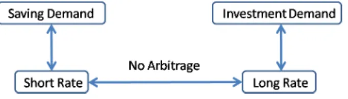
2of liquidity preference, the interest rate elastic component, stems out of the speculative motive. Keynes defines the speculative motive as ’the object of securing profit from knowing better than the market what the future will bring forth (Keynes (1936, page 170) )’, for exam- ple an ‘individual, who believes that future rates of interest will be above the rates assumed by the market, has a reason for keeping actual liquid cash’ (Keynes (1936, page 170)). In other words, speculative money demand is due to speculation on higher long term interest rates and lower bond prices. This fits to the intuition which drives the argument in Chapter 2. Here, investors speculate on better future investment opportunities which is why they demand short term rather than long term assets, should long term yields be too low compared to rates that can be rationally expected for the future. Thereby, short term rates can drop below zero although the marginal product of capital is strictly positive. But while Keynes speculative motive is due to believes which deviate from market expectations and therefore based on either a market inefficiency or on heterogeneous expectations, the model in Chapter 2 relies on a no-arbitrage condition as connection between the long rate an short rate dynam- ics. It is based on rational expectations and therefore consistent with neo-classical thinking.
Thinking about Keynes’ theory and the speculative motive in particular, naturally leads to questions linked to liquidity preference. Can the model rationalize a liquid- ity trap? What exactly is a liquidity trap? Is monetary policy really powerless when short term rates are near or below zero, or are there remedies? Regrettably, these questions are far too ambitious to be answered based on the model of Chapter 2.
More elementary questions have to be answered first. It is the believe of the author that while introducing a role for money in an ad hoc way (e.g. by postulating a cash-in advance-constraint or putting money in the utility function) allows to pro- duce numbers, but does not contribute to a meaningful monetary analysis as long as the role that money plays in the real world is not cleared. So what exactly is money (what is liquidity)?
The third and last chapter, ’Why Fiat Money is a Safe Asset’, attempts to make one first step towards answering this question. It asks: Why do people exchange real goods against a piece of paper that neither provides intrinsic utility nor (unlike in Keynes times) constitutes a claim on a real good such as gold? Why is money a safe asset whose value people (can) rely upon?. In the model presented in Chapter 3, a slightly extended version published in Economics Letters (Paulsen (2012)), money is
’safe’: Fiat money has strictly positive value in the unique trembling hand equilibrium.
This holds as each bank note is both: a witness for the existence of some agent in the economy with debt, backed by collateral, and the only matter that allows the debtor to settle her debt. Debtors fear to lose the collateral and compete with each other for not defaulting, i.e. they compete for money. This creates money demand
2Without interest rate elasticity of money demand Keynes theory would collapse to the ’classic’
quantity theory.
and thereby ensures positive money value. As not only a single but all debtors in the economy demand money, idiosyncratic shocks to solvency wash out. This makes fiat money a safe asset.
References
K. Back and D. Paulsen Open-loop equilibria and perfect competition in option exercise games strategies of firms. Review of financial studies, 22(11):4531–4552, 2009.
A.K. Dixit and R.S. Pindyck. Investment under uncertainty. Princeton Univ Pr, 1994.
S.R. Grenadier. Option exercise games: An application to the equilibrium investment strategies of firms. Review of financial studies, 15(3):691–721, 2002.
John M. Keynes. The general theory of employment, interest and money. 1936.
J.V. Leahy. Investment in competitive equilibrium: The optimality of myopic behav- ior. The Quarterly Journal of Economics, 108(4):1105–1133, 1993.
D. Paulsen. Why fiat money is a safe asset. Economics Letters, 116(2):193–198, 2012.
This page is intentionally left blank.
1. OPEN-LOOP EQUILIBRIA AND PERFECT COMPETITION IN OPTION EXERCISE GAMES
Abstract
The investment boundaries defined by Grenadier (2002) for an oligopoly investment game determine equilibria in open loop strategies. As closed loop strategies, they are not equilibria, because any firm by investing sooner can preempt the investments of other firms and expropriate the growth options. The perfectly competitive outcome is produced by closed loop strategies that are mutually best responses. In this equi- librium, the option to delay investment has zero value, and the simple NPV rule is followed by all firms.
JEL classification: C73, D43, D92, G31, L13 Keywords:
1.1 Introduction
This paper analyzes oligopoly investment under uncertainty, assuming capital invest- ment is irreversible and capital stocks are instantaneously adjustable upward at a fixed price of capital. This oligopoly model is analyzed by Baldursson (1998) and Grenadier (2002). A similar model is analyzed by Leahy (1993) and Baldursson and Karatzas (1996) under the assumption of perfect competition and by Abel and Eberly (1996) and Merhi and Zervos (2005) under the assumption of monopoly. The investment policies described by all of these authors are singular, meaning that the investment rate is zero almost everywhere and undefined when investment occurs.
The oligopoly model has important implications for the value of the option to delay investment – and hence the cost of ignoring this option and using the simple NPV rule for project choice – and may also be useful for understanding the dynamics of risk and return in equilibrium (see Novy-Marx (2007)).
The equilibrium concept in Baldursson (1998) is Nash, and strategies are stochastic processes adapted to the exogenous process that influences demand. This is an “open loop” concept, in the sense that there is no feedback from the investment of any firm to the investment of any other firm. It appears that Grenadier presents an equilib- rium in closed loop strategies, but this is misleading. We show that his equilibrium is also open loop.
The distinction between open loop and closed loop (or feedback) strategies is well understood in the context of deterministic oligopoly investment games. See Fersht- man and Muller (1984), Reynolds (1987), Tirole (1988), or Fudenberg and Tirole (1992). Equilibria in open loop strategies are unattractive because they fail subgame or Markov perfection. Open loop strategies are commitments to invest, depending on the history of demand in the stochastic context, regardless of the investments of other firms, even though there is no device in the game to make such commitments credible.
For example, in an open loop equilibrium, if one firm deviates to invest more than the equilibrium strategy specifies, driving the price down, other firms ignore this and continue to invest as they would have. This is inconsistent with subgame perfection.
1There are difficulties in even defining the game in closed loop form. To do so would seem to require an extension of Simon and Stinchcombe’s (Simon and Stinch- combe, 1989) analysis of deterministic continuous-time games with finite action sets to stochastic continuous-time games with continuum action sets. However, it is possible to show that the closed loop “trigger strategies” of Grenadier (2002) are not mutually best responses. By investing earlier, any firm can preempt the investments of other firms. To do so reduces the aggregate value of growth options but allows the preempt- ing firm to expropriate growth options. We show that this tradeoff favors preemption.
Trigger strategies employing the perfectly competitive trigger (i.e., following the sim-
1More precisely, it is inconsistent with subgame perfection if each firm observes the output price and hence has at least partial information about other firms’ outputs.
ple NPV rule) are mutually best responses. If one firm’s strategy is to invest enough to ensure that aggregate industry capital equals the capital stock of a perfectly com- petitive industry, then any other firm might as well employ the same strategy. This is an extreme form of Reynolds’s (Reynolds, 1987) observation in a deterministic model with quadratic adjustment costs that closed loop equilibria involve higher steady- state capital stocks than open loop equilibria, because “the preemptive or strategic element of investment behavior in the feedback Nash equilibrium influences the long run market outcome.”
Perfect competition is of course also the outcome of Bertrand competition, so one might conjecture that playing the perfectly competitive trigger is implicitly compe- tition in prices. We believe that this is the wrong interpretation. The game is one of competition in quantities (capital stocks). However, modeling time as continuous means that firms can instantaneously respond to others’ investment choices. The basic assumption of the model is that arbitrarily large investments can be made in- stantaneously with no adjustment cost other than the fixed price of capital. Thus, at each instant in time, the game can be viewed as one of Stackelberg competition, in which each firm chooses its investment with all other firms instantaneously following.
Naturally, each firm aspires to be the Stackelberg leader. A stable point, perhaps the only stable point, of this joint Stackelberg leadership is perfect competition.
The first author would like to note that his prior sole-authored working paper on this topic was excessively critical of Grenadier’s concept of a myopic firm. That concept is indeed useful — to derive an open loop equilibrium. We prove that conditions sim- ilar to those in Grenadier’s Proposition 3 are sufficient conditions for an open loop equilibrium.
The proof of open loop equilibrium is in Section 2. Section 3 discusses the difficulties with defining the game in closed loop form, the fact that the trigger strategies of Grenadier (2002) are not best responses to each other, and the fact that playing the perfectly competitive triggers are mutually best responses. Section 4 briefly concludes.
1.2 Open Loop Equilibrium
There are n firms in the industry. There is a constant required rate of return r.
The capital stock of firm i at date t is denoted by Q
it, and we set Q
−it=
Pj6=i
Q
jt. The cost of a unit of capital is normalized to 1. Capital does not depreciate, and investment is irreversible.
Consider a filtered probability space (Ω, (F
t)
t≥0,
P) and a one-dimensional standard Brownian motion B on the probability space. Let X be a solution of a stochastic differential equation
dX
t= µ(X
t) dt + σ(X
t) dB
t. (1.1) Assume σ(X
t)
6= 0 for allt almost surely. Define the running maximum
X
t∗= max
0≤s≤t
X
s.
Assume that the operating cash flow rate of firm i at date t depends on X
t, Q
itand Q
−it. Denote it by π(X
t, Q
it, Q
−it). Assume that π is twice continuously differentiable in (x, q
i, q
−i), increasing in x, and concave in q
i.
Denote marginal operating cash flow by ζ(x, q
i, q
−i) = ∂
∂q
iπ(x, q
i, q
−i) .
Assume ζ
q−i ≥ζ
qiand ζ
q−i(x, 0, q
−i)
≤0, where the subscripts denote partial deriva- tives. Though it is not required, we could take
π(x, q
i, q
−i) = P (x, q
i+ q
−i)q
i−C(q
i)
for some functions P and C. In that case, P
q ≤0 and C
00 ≥0 imply ζ
q−i ≥ζ
qi. Assume further that ζ is increasing in x and that the integrability constraint
E Z ∞
0
e
−rtsup
a≤q−i≤b
|ζ(Xt
, q
i, q
−i)|dt <
∞. (1.2) is satisfied for each fixed triple (q
i, a, b).
2Denote the initial capital stock of firm i by q
i0. The set of admissible open loop strategies of firm i is
A(qi0
) =
{(Qit)
t≥0 |nondecreasing, left-continuous,
Ft-adapted, Q
i0 ≥q
i0}. (1.3) If each firm j
6=i plays an open loop strategy, then the stochastic process Q
−iis an exogenous
Ft-adapted process from the point of view of firm i. Firm i chooses Q
i ∈ A(qi0) to maximize
Π(Q
i, Q
−i) =
E Z ∞0
e
−rt[π(X
t, Q
it, Q
−it) dt
−dQ
it] . (1.4) An open loop equilibrium — i.e., a Nash equilibrium in open loop strategies — is an n-tuple (Q
∗1, . . . , Q
∗n) of admissible strategies such that, for each i,
Q
∗i ∈argmax
Qi∈A(qi0)Π(Q
i, Q
∗−i) . (1.5) The function m described in the proposition below should be interpreted as a marginal value function (marginal with respect to q
i). It is also the value function of the optimal stopping problem (1.9) defined below. The hypotheses of the proposition are similar to those in Grenadier’s Proposition 3, though Grenadier’s assumptions regard the functions
(x, q)
7→m(x, q, (n
−1)q) and q
7→X(q, (n
−1)q) ,
i.e., the values of m and X along a ray in the (q
i, q
−i) domain, whereas our assumptions concern m and X on their entire domains. The conclusion differs regarding the nature of equilibrium — open loop instead of closed loop. The proposition is proven in Appendix 1.5.
2The integrability constraint is used to deduce convergence of expectations in the proof of Propo- sition 1. It can be replaced byζ≥0, using the monotone convergence theorem in the proof.
Proposition 1.2.1.
Suppose there exist functions m(x, q
i, q
−i) and X(q
i, q
−i) satis- fying the following conditions:
1. X(q
i, q
−i) is differentiable in q
−iand continuous in q
i. 2. X(q
i, q
−i) and X(q
i, (n
−1)q
i) are increasing in q
i.
3. m is bounded from below for each fixed pair (q
i, q
−i), twice continuously differ- entiable with respect to x, and once continuously differentiable with respect to (q
i, q
−i).
4. m is monotonically increasing in x for x
≤X(q
i, q
−i).
5. m solves the PDE
µm
x+ 1
2 σ
2m
xx−rm + ζ = 0 (1.6)
on the region x < X (q
i, q
−i).
6. m(X(q
i, q
−i), q
i, q
−i) = 1 (value matching).
7. m
x(X(q
i, q
−i), q
i, q
−i) = 0 (smooth pasting).
Then the following are true:
(A) Myopic Optimality. If Q
jt= q
j0for all j
6=i and all t
≥0, then
Q
it= inf
{qi ≥q
i0 |X
t∗ ≤X(q
i, q
−i0)} (1.7) maximizes (1.4) over Q
i ∈ A(qi0).
(B) Symmetric Open Loop Equilibrium. Suppose q
i0= q
j0for all i and j . Then (Q
∗1, . . . , Q
∗n) is an open loop equilibrium, where, for each i,
Q
∗it= inf
{qi ≥q
i0 |X
t∗ ≤X(q
i, (n
−1)q
i)} . (1.8) Assumptions 3–7 ensure that the function m fulfills the criteria of a Hamilton-Jacobi- Bellman verification theorem for the optimal stopping problem
min
τ E Z τ0
e
−rtζ(X
t, q
i, q
−i)dt + e
−rτ. (1.9)
More precisely, m is the value function of this stopping problem, and the hitting time of the boundary X(q
i, q
−i) is an optimal stopping rule. The optimal stopping problem can be interpreted as the problem of a firm to optimally install a unit of capital un- der the myopic assumption that rival firms will never do so and that no further unit can be installed. In the formulation (1.9), the firm minimizes the opportunity cost (the foregone marginal cash flow) of not investing plus the discounted cost of investing.
The smooth pasting condition deserves a comment. Heuristically it can be derived by
the envelope theorem. Namely, let M (x, y ) be the expected value in (1.9) when X
0= x
and the stopping time is the first hitting time of y. By the value matching condition, M (y, y) = 1, so differentiating this with respect to y yields M
x(y, y) + M
y(y, y) = 0.
However, if y
∗is optimal, then M
y(·, y
∗) should equal zero. So M
x(y
∗, y
∗) = 0 at the optimal boundary y
∗.
There is a large literature on the connection between singular stochastic control prob- lems and optimal stopping problems, starting with Karatzas and Shreve (1984). The equivalence between the control problem and the stopping problems here is the same as in Theorem 1 of Bank (2006). What is new about our proof, as far as we know, is the solution of the stopping problems in the presence of the exogenous singular process Q
−i.
Now we apply Proposition 1.2.1 to the linear model studied by Baldursson and Karatzas (1996) and the constant elasticity example considered by Grenadier (2002).
Grenadier and Baldursson present the value of X(q
i, q
−i) when q
−i= (n
−1)q
i. The entire function X(q
i, q
−i) is presented below.
Constant Elasticity
Assume π(x, q
i, q
−i) = P (x, q
i+ q
−i)q
iwith P (x, q) = xq
−1/γ. Assume γ > 1. Assume X is a geometric Brownian motion with parameters µ and σ; i.e., µ(x) = µx and σ(x) = σx with a slight abuse of notation. Assume r > µ and β > γ, where
β =
−µ
− 12σ
2+
q
µ
−12σ
22+ 2rσ
2σ
2. (1.10)
These restrictions on the parameters imply that the model satisfies our assumptions regarding π. We have
ζ(x, q
i, q
−i) =
1
−q
iγ(q
i+ q
−i)
x(q
i+ q
−i)
−1/γ.
Proposition 1.2.2.
In the constant elasticity model, there is a unique pair (m, X) satisfying the conditions of Proposition 1,
3and
X(q
i, q
−i) = β β
−1
γ
γ
−q
i/(q
i+ q
−i)
(r
−µ)(q
i+ q
−i)
1γ, (1.11a) m(x, q
i, q
−i) = ζ(x, q
i, q
−i)
r
−µ
−ζ(X(q
i, q
−i), q
i, q
−i) (r
−µ)β
x X(q
i, q
−i)
β
. (1.11b) Proof. The general solution to the PDE (1.6) is
m(x, q
i, q
−i) = ζ(x, q
i, q
−i)
r
−µ + Ax
β+ Bx
β0with β given by (1.10), and β
0= 1
−β
−2µ/σ
2< 0. Assumptions 3 and 4 imply m is bounded in x on the interval (0, X (q
i, q
−i)), so B = 0. Solving conditions 6 and 7 in the unknowns A and X(q
i, q
−i) yields (1.11).
3Uniqueness ofmis on the domain{(x, qi, q−i)|x≤X(qi, q−i)}.
Linear Demand
Assume π(x, q
i, q
−i) = P (x, q
i+q
−i)q
i−cqi, with P (x, q) = x−bq, for constants b and c.
Assume X is a geometric Brownian motion with parameters µ and σ. Assume β > 2, where β is defined in (1.10). Then the model satisfies our assumptions regarding π.
We have ζ(x, q
i, q
−i) = x
−2bq
i−bq
−i−c.
Proposition 1.2.3.
In the linear model, there is a unique pair (m, X ) satisfying the conditions of Proposition 1.2.1, and
X(q
i, q
−i) = β β
−1
r
−µ r
(c + r + 2bq
i+ bq
−i) , (1.12a) m(x, q
i, q
−i) =
−2bqi−bq
−i−c
r + x
r
−µ
−x
β(r
−µ)βX (q
i, q
−i)
β−1. (1.12b) Proof. The general solution to the PDE (1.6) is:
m(x, q
i, q
−i) = ζ(x, q
i, q
−i)
r + Ax
β+ Bx
β0with β as given in (1.10) and β
0= 1
−β
−2µ/σ
2< 0. For the same reasons as in the constant elasticity case, B = 0. Solving the smooth pasting and the value matching condition for A and X yields (1.12).
1.3 Closed Loop Strategies and Best Responses
First, we admit we do not know how to define this game in closed loop form. There are substantial complications in doing so. If the capital stock processes were absolutely continuous instead of singular, one would view the investment rate z
it= dQ
it/dt as the decision variable of firm i at date t. If each z
itwere required to depend on the history of (X, Q
1, . . . , Q
n) prior to t in a sufficiently regular way, then the capital stock processes
Q
it= q
i0+
Z t0
z
itdt
would be well defined. With singular controls, one could view the action of firm i at any date t as being the Lebesgue-Stieltjes differential dQ
itof its capital stock process Q
i; however, these differentials are meaningful only in integrated form. An alternate view is that the action of firm i at date t is its total capital Q
it, chosen subject to the constraint that capital is irreversible: Q
it ≥sup
s<tQ
is. However, this suffers from the general problem with continuous-time games that what seem to be well-defined strategies may not produce well-defined outcomes (see Simon and Stinchcombe, 1989).
For example, the formula Q
it= sup
s<tQ
isseems to specify Q
itas a function of the
history of play prior to t; yet, every nondecreasing left-continuous process Q
isatis-
fies the formula. Likewise, the formulas Q
it= lim
s↑tQ
jsand Q
jt= lim
s↑tQ
isseem
to define each firm’s capital stock at time t as a function of the other firm’s prior
investments, but these formulas are satisfied by every left-continuous Q
i= Q
j. Thus,
formulas such as these — and one could give an arbitrary number of similar examples
— are very far from uniquely specifying how the game is to be played. In order to define the game, some rules must be constructed to allow one to map such formulas, or whatever strategies are allowed, into unique outcomes. Simon and Stinchcombe (1989) accomplish this for deterministic games with finite action sets. Generalizing their work to the present context, and then finding equilibria, would seem to be sub- stantial tasks.
Though we do not know how to define strategies in general, there are some com- binations of decision rules that clearly produce well-defined outcomes. Grenadier’s Proposition 1 states: “Each firm’s investment strategy is characterized by increas- ing output incrementally whenever X(t) rises to the trigger function ¯ X(q
i, Q
−i).”
4Though Grenadier’s statement is not a precise description of a strategy, it seems reasonable to take its meaning to be
Q
it= inf
q
i ≥q
i0
sup
0≤s≤t
[X
s−X(q
i, Q
−is)]
≤0
. (1.13)
Given a stochastic process Q
−i, this defines Q
ias the smallest nondecreasing pro- cess such that X
t ≤X(Q
it, Q
−it) for all t. Note that Q
itis allowed to depend on the contemporaneous Q
−it. This seems reasonable for all t > 0 if we restrict to left-continuous paths.
5Decision rules of the form (1.13) do not necessarily produce well-defined outcomes. For example, in a two-firm game, if both firms play (1.13) for X(q
i, q
−i) = q
i+ q
−i, then the division of output between the two firms is not defined. However, if all firms play (1.13) for the open loop equilibrium investment boundaries in the constant elasticity and linear examples — i.e., for X defined in (1.11a) or (1.12a) — then the capital paths of all firms are well defined. In fact, the strategies (1.13) with the open loop equilibrium investment boundaries produce the open loop equilibrium capital processes.
If all firms play (1.13) for an increasing X(·) and the paths are well defined, then any firm can preempt the investments of other firms by investing aggressively itself. The following proposition shows that the open loop equilibrium boundary in the linear model does not define a closed loop equilibrium, because preemption is a profitable deviation (the strategies (1.14) and (1.15b) are the strategies asserted by Grenadier to constitute an equilibrium in the linear model).
Proposition 1.3.1.
Suppose X is a geometric Brownian motion with drift µ and volatility σ. Assume π(x, q
i, q
−i) = (X
−b(q
i+ q
−i)
−c)q
ifor constants b > 0 and c
≥0. Assume q
i0= q
j0for all i and j, and define q
0=
Pni=1
q
i0. Assume β > 2,
4X(q¯ i, Q−i) equals the myopic triggerX(qi, Q−i) from Proposition 1.2.1 (see Grenadier’s Propo- sition 2).
5If X0 > X(qi0, q−i0), then (1.13) implies a jump at time 0. It allows this jump to depend on simultaneous jumps of other firms. This seems unreasonable, but one could view it as a reduced form for nearly instantaneous reactions. Simon and Stinchcombe (1989) discuss this issue.
where β is defined in (1.10). Assume for all j
6=i that Q
jt= inf
q
j ≥q
j0sup
0≤s≤t
X
s−β β
−1
r
−µ r
(c + r + 2bq
j+ bQ
−js)
≤
0
.
(1.14) Define
τ = inf
t
≥0
X
t∗ ≥β β
−1
r
−µ
r c + r + (n + 1)bq
0n .
There exists α > 1 such that the open loop strategy Q
αit=
(
q
i0for t
≤τ , inf
nq
i ≥αq
i0 |X
t∗ ≤ β−1β r−µrc + r +
n+ααbq
iofor t > τ , (1.15a) produces higher expected discounted cash flows for firm i than does the closed loop strategy
Q
it= inf
q
i ≥q
i0sup
0≤s≤t
X
s−β β
−1
r
−µ r
(c + r + 2bq
i+ bQ
−is)
≤
0
.
(1.15b) Proof. The unique n–tuple (Q
1, . . . , Q
n) of stochastic processes satisfying (1.14) and (1.15b) is the open loop equilibrium (Q
∗1, . . . , Q
∗n) defined in Proposition 1 and Propo- sition 1.2.3. Let α
≥1. The unique n–tuple (Q
1, . . . , Q
n) of stochastic processes satisfying (1.14) and (1.15a) is (Q
α1, . . . , Q
αn), where Q
αiis defined in (1.15a) and
(∀ j
6=i) Q
αjt=
(
q
j0for t
≤τ ,
Q
αit/α for t > τ . (1.16) To see this, note that the equality of the Q
jfor j
6=i implies Q
−jt= (n
−2)Q
jt+ Q
αit. Making this substitution in (1.14), we have
Q
jt= max
q
j0, sup
0≤s≤t
1 nb
β
−1 β
r r
−µ
X
s−c
−r
−bQ
αis. (17a)
Moreover, (1.15a) implies, for t > τ, Q
αit= α max
q
i0, 1 (n + α)b
β
−1 β
r r
−µ
X
t∗−c
−r
. (17b)
Substituting (17b) in (17a) yields (1.16).
Note that, for α = 1, Q
αj= Q
∗jfor all j = 1, . . . , n. Define F (α) = Π(Q
αi, Q
α−i),
where Π(·) is the expected discounted cash flow defined in (1.4). The claim is that
F (α) > F (1) for some α > 1. We show in Appendix B that the right-hand derivative
of F at α = 1 is positive. Thus, F (α) > F (1) for all sufficiently small α > 1.
The preemption strategy (1.15a) involves a limited amount of preemption: jumping to a market share of α/(n + α
−1) and maintaining that market share forever. For some parameter values in the linear model, expropriating all of the growth options is a profitable deviation from (1.15b). To explain what it means to expropriate all of the growth options, consider the constant elasticity example and the boundary (1.11a).
Note that q
iq
i+ q
−i→
0
⇒X(q
i, q
−i)
→β
β
−1 (r
−µ)(q
i+ q
−i)
1γ. (1.18) The limit of X(q
i, q
−i) displayed in (1.18) is the perfectly competitive investment boundary defined by Leahy (1993). It is the boundary at which a firm with infinites- imal market share would invest. Thus, if some firm j plays (1.13), i.e.,
Q
jt= inf
q
j ≥q
j0sup
0≤s≤t
[X
s−X(q
j, Q
−js)]
≤0
, (1.19)
then the behavior of firm j will approach that of a perfectly competitive firm as its market share decreases. If firm i invests sufficiently aggressively that it deters the investments of other firms, then the market shares of other firms will gradually de- cline toward zero, and their behavior under the decision rule (1.19) with boundary (1.11a) will approach that of perfect competition. Thus, aggregate output and price will approach the perfectly competitive output and price, and the value of industry growth options will eventually be destroyed. In exchange for this diminution of in- dustry growth options, the preempting firm can expropriate all growth options to itself. We have calculated, though it is not presented here, that expropriating all of the growth options is a profitable deviation from (1.15b) in the linear model for some parameter values. Paulsen (2006) shows that preempting for a finite period of time is a profitable deviation in the constant elasticity model for some parameter values.
The perfectly competitive boundary is immune to preemption. Suppose, in the con- stant elasticity example, that each firm plays
Q
it= inf
q
i ≥q
i0sup
0≤s≤t
X
s−β
β
−1 (r
−µ)(q
i+ Q
−is)
1γ≤
0
. (1.20) Given symmetric initial conditions and initial industry capital q
0, equation (1.20) holds for each i whenever the Q
iare nondecreasing processes such that industry capital Q
t=
Pni=1
Q
itsatisfies Q
t= inf
q
≥q
0 |X
t∗ ≤β
β
−1 (r
−µ)q
γ1.
Thus, (1.20) suffers from the problem discussed in the first paragraph of this section:
It does not produce well-defined individual firm capital processes. However, it does
produce well-defined individual firm values, which is the key requirement for choosing
among strategies. Because industry growth options have zero value when investing
at the perfectly competitive boundary, it does not matter how growth is distributed among the firms. Moreover, if all other firms play (1.20), then it is optimal for each individual firm to play (1.20), because the price process is unaffected by an individ- ual firm playing (1.20) when other firms also play (1.20), and the investments from playing (1.20) are zero NPV when the price process is taken as given. The only sub- optimal decision a firm could make when other firms play (1.20) is to invest before the perfectly competitive boundary is reached, and this does not occur when a firm plays (1.20). Thus, the strategies (1.20) are mutually best responses.
Though the strategies (1.20) are choices of quantities, not prices, the outcome is like Bertrand in that the “economic value added” of each firm is zero. Related to this is another feature the equilibrium shares with Bertrand: the strategies are weakly dominated. Investing zero at all times is as valuable as making zero NPV investments, and it is superior to playing (1.20) if other firms play investment strategies that are less aggressive than (1.20).
1.4 Conclusion
Open loop equilibria have an extreme Cournot nature: Each firm optimizes taking the entire output process of each other firm as given. They fail subgame perfection, because if a firm invests aggressively the game will reach a node from which the given output processes of other firms will not be part of a Nash equilibrium starting from that node. The closed loop strategies (1.13) have the potential to form subgame per- fect equilibria, because each firm reacts to the investments of others. These strategies have a Stackelberg flavor, because all firms react to the investments of any firm like Stackelberg followers, and hence each firm is like a Stackelberg leader. A stable point of this joint Stackelberg leadership is perfect competition.
The closed loop strategies (1.13) employing the myopic (open loop equilibrium) boundary do not form an equilibrium, because any firm by investing more can cause other firms to invest less, like a Stackelberg leader, and hence expropriate some of the growth options. We proved that this preemptive investment is a profitable deviation in the linear model. Paulsen (2006) shows the same for the constant elasticity model, for some parameter values.
It is an open question whether the perfectly competitive boundary is the unique boundary such that closed loop strategies of the form (1.13) are impervious to pre- emption. If so, the perfectly competitive boundary would be the unique boundary such that the strategies (1.13) could constitute an equilibrium.
It seems likely that there would be other closed-loop equilibria, if the strategy spaces
and mapping from strategy n–tuples to outcomes could be specified. There should
be equilibria in punishment strategies, in which firms invest less than the perfectly
competitive amount and threaten to punish any firm that deviates. These strategies
are not of the form: invest when X
t= X(Q
it, Q
−it) for an increasing function X, be-
cause strategies of this form prescribe less investment when competitors invest more
and hence do not allow for punishment.
Appendix
1.5 Proof of Proposition 1.2.1
Define
¯
m(x, qi, q−i) =
(m(x, qi, q−i) ifx≤X(qi, q−i),
1 otherwise. (1.5.1)
Lemma 1.5.1. m¯q−i(x, qi, q−i) = 0 forx≥X(qi, q−i).
Proof. By the value-matching condition, we have
¯
m(X(qi, q−i), qi, q−i) = 1. Differentiating this equation with respect toq−i yields
¯
mx(X(qi, q−i), qi, q−i)Xq−i(qi, q−i) + ¯mq−i(X(qi, q−i), qi, q−i) = 0. As the first term vanishes by the smooth-pasting condition, we get
¯
mq−i(X(qi, q−i), qi, q−i) = 0.
This proves the claim forx=X(qi, q−i). Forx > X(qi, q−i), ¯m(x, qi, z) = 1 forzin a neighborhood ofq−i by definition of ¯m. Hence, differentiation yields the result.
Lemma 1.5.2. We have (for allx6=X(qi, q−i))
−rm¯ +µm¯x+1
2σ2m¯xx≥ −ζ with equality forx < X(qi, q−i).
Proof. Forx < X(qi, q−i) equality holds by Assumption 5 of Proposition 1.2.1. Assumptions 4 and 7 imply thatmxx≤0 forx=X(qi, q−i). Therefore
−rm+µmx≥ −ζ atx=X(qi, q−i). Using the smooth pasting condition we get
−rm¯ =−rm≥ −ζ
atx=X(qi, q−i). Note thatζ increases inxwhile ¯mremains constant, so
−rm¯ +µm¯x+1
2σ2m¯xx=−rm¯ + 0 + 0≥ −ζ forx > X(qi, q−i).
Consider the myopic problem indexed byy=qi0 andz=q−i0: max
Qi∈A(y) E Z ∞
0
e−rt(π(Xt, Qit, z)dt−dQit). (1.5.2) Related to this problem is the following optimal stopping problem: Choose a stopping time τ to maximize
E Z ∞
τ
e−rtζ(Xt, y, z)dt−e−rτ
=E Z ∞
τ
e−rt(ζ(Xt, y, z)−r)dt
. (1.5.3)
To interpret the optimal stopping problem, notice that a small investment at time τ increases expected discounted revenues by approximately
·E Z ∞
τ
e−rtζ(Xt, y, z)dt
and has expected discounted cost equal to ·E[e−rτ]. The optimal stopping time is therefore the optimal time to make a investment of size ≈ 0. Subtracting ER∞
0 e−rtζ(Xt, y, z)dt and multiplying by (−1) converts the problem of maximizing (1.5.3) to the following equivalent problem:
minτ E Z τ
0
e−rtζ(Xt, y, z)dt+e−rτ
. (1.5.4)
This can be interpreted as minimizing the opportunity cost of a unit of capital.
We also consider the equilibrium problem indexed by y =qi0 and z = q−i0. In this problem, we assume the aggregate capital of firmsj6=iis
Lzt= inf
q≥z| max
0≤s≤tXs≤X(q/(n−1), q)
. (1.5.5)
The optimization problem for firmithat we study is:
max
Qi∈A(y) E Z ∞
0
e−rt(π(Xt, Qit, Lzt)dt−dQit). (1.5.6) The related optimal stopping problem is: Choose a stopping timeτ to maximize
E Z ∞
τ
e−rtζ(Xt, y, Lzt)dt−e−rτ
=E Z ∞
τ
e−rt(ζ(Xt, y, Lzt)−r)dt
, (1.5.7)
which is equivalent to:
minτ E Z τ
0
e−rtζ(Xt, y, Lzt)dt+e−rτ
. (1.5.8)
For anyy andz, define
τyz = inf{t|Xt> X(y, z)}. (1.5.9) Lemma 1.5.3. τyz solves the myopic stopping problem (1.5.4).
Proof. By an approximation argument as in Øksendal (2002) (see Theorem 10.4.1), we can assume that ¯mis twice continuously differentiable with respect tox. Letτ be an arbitrary stopping time.
Applying Itˆo’s rule toe−r(t∧τ)m(X¯ t∧τ, y, z) yields:
e−r(t∧τ)m(X¯ t∧τ, y, z) = ¯m(X0, y, z) + Z t∧τ
0
e−rsm¯xσ dBs +
Z t∧τ 0
e−rs(−rm¯ +µm¯x+1
2σ2m¯xx)ds . (1.5.10) Applying Lemma 1.5.2 to (1.5.10), we get
e−r(t∧τ)m(X¯ t∧τ, y, z) ≥ m(X¯ 0, y, z) + Z t∧τ
0
e−rsm¯xσ dBs
− Z t∧τ
0
e−rsζsds ,
with equality for τ ≤τyz. We cannot directly take expectations on both sides as we do not know whether the stochastic integral is a martingale or just a local martingale. So letτk ≤kbe a localizing
sequence for the stochastic integral. That is, τk ↑ ∞ and the stopped integrals are martingales.
Taking expectations on both sides and using Doob’s optional sampling theorem yields, for eachk, E
h
e−r(τk∧τ)m(X¯ τk∧τ, y, z)i
≥ m(X¯ 0, y, z)−E
Z τk∧τ 0
e−rsζsds
.
Observe that ¯mis bounded from above by 1 and bounded from below by Assumption 3 in Proposition 1.2.1, whereas the integrals involvingζare uniformly integrable by the integrability assumption (1.2).
Taking the limitk→ ∞we get
¯
m(X0, y, z) ≤ lim
k→∞E h
e−r(τk∧τ)m(X¯ τk∧τ, y, z)i + lim
k→∞E
Z τk∧τ 0
e−rsζsds
= E
e−rτm(X¯ τ, y, z) +E
Z τ 0
e−rsζsds
, or
¯
m(X0, y, z) ≤ E Z τ
0
e−rsζsds
+E
e−rτm(X¯ τ, y, z)
≤ E Z τ
0
e−rsζsds
+E e−rτ
, with equality forτ=τyz.
Lemma 1.5.4. Ify=z/(n−1), then τyz solves the equilibrium stopping problem (1.5.8).
Proof. We proceed as in the proof of Lemma 1.5.3 with the difference that nowdLzt6= 0. Letτ be an arbitrary stopping time. Applying Itˆo’s rule toe−r(t∧τ)m(X¯ t∧τ, y, Lz,t∧τ) yields:
e−r(t∧τ)m(X¯ t∧τ, y, Lt∧τ,z) = ¯m(X0, y, z) + Z t∧τ
0
e−rsm¯xσ dBs
+ Z t∧τ
0
e−rs(−rm¯ +µm¯x+1
2σ2m¯xx)ds+ Z t∧τ
0
e−rsm¯q−idLzs. (1.5.11) Note thatLincreases only whenXt=X(Lzt/(n−1), Lzt). We have Lzt/(n−1)≥z/(n−1) =y.
By monotonicity ofX, it follows thatLincreases only whenXt≥X(y, Lzt). In this case, Lemma 1 implies
¯
mq−i(Xt, y, Lzt)dLzt= 0. (1.5.12) Applying (1.5.12) and Lemma 2 to (1.5.10), we get
e−r(t∧τ)m(X¯ t∧τ, y, Lz,t∧τ) ≥ m(X¯ 0, y, z) + Z t∧τ
0
e−rsm¯xσ dBs
− Z t∧τ
0
e−rsζsds ,
with equality for τ ≤τyz. As in the proof of Lemma 1.5.3 we take a localizing sequence τk ≤ k.
Taking expectations on both sides yields, for eachk:
E
he−r(τk∧τ)m(X¯ τk∧τ, y, Lz,τk∧τ)i
≥m(X¯ 0, y, z)−E
Z τk∧τ 0
e−rsζsds
.
Observe that ¯mis bounded from above by 1 andζ(Xs, y, Lzs)≤ζ(Xs,0, Lzs)≤ζ(Xs,0, z) which is integrable by assumption (1.2). So applying Fatou’s lemma yields:
¯
m(X0, y, z) ≤ lim sup
k→∞ E
h
e−r(τk∧τ)m(X¯ τk∧τ, y, Lz,τk∧τ)i
+ lim sup
k→∞ E
Z τk∧τ 0
e−rsζsds
≤ E
e−rτm(X¯ τ, y, Lzτ) +E
Z τ 0
e−rsζsds
; (1.5.13)