Robust estimation methods with application to flood statistics

DISSERTATION

in partial fullment of the requirements for the degree of Doktor der Naturwissenschaften

Robust estimation methods with application to ood statistics

Svenja Fischer

born on 02.07.1989 in Recklinghausen

August 2017

Advisors: Prof. Dr. A. Schumann, Prof. Dr. M. Wendler, Prof. Dr. R.

Fried

Reviewers: Prof. Dr. R. Fried, Prof. Dr. W. Krämer, Prof. Dr. M.

Wendler, Prof. Dr. A. Schumann

Robust statistics and the use of robust estimators have come more and more into focus during the last couple of years. In the context of ood statistics, robust estimation methods are used to obtain stable estimations of e.g. design oods. These are estimations that do not change from one year to another just because one large ood occurred.

A problem which is often ignored in ood statistics is the underlying dependence structure of the data. When considering discharge data with high time-resolution, short range dependent behaviour can be detected within the time series. To take this into account, in this thesis a limit theorem for the class of GL-statistics is developed under the very general assumption of near epoch dependent processes on absolutely regular random variables, which is a well known concept of short range dependence. GL-statistics form a very general class of statistics and can be used to represent many robust and non-robust estimators, such as Gini's mean dierence, the Q_n-estimator or the generalized Hodges-Lehmann estimator. In a direct application the limit distribution ofL-moments and their robust extension, the trimmedL-moments, is derived.

Moreover, a long-run variance estimator is developed. For all these results, the use ofU-statistics andU-processes proves to be the key tool, such that a Central Limit Theorem for multivariateU- statistics as well as an invariance principle forU-processes and the convergence of the remaining term of the Bahadur-representation for U-quantiles is shown. A challenge for proving these results pose the multivariate kernels that are considered to be able to represent very general estimators and statistics.

A concrete application in the context of ood statistics, in particular in the estimation of design oods, the classication of homogeneous groups and the modelling of short range dependent discharge series, is given. Here, well known models (peak-over-thresholds) as well as newly developed ones, for example mixing models using the distinction of oods according to their timescales, are combined with robust estimators and the advantages and disadvantages under consideration of stability and eciency are investigated. The results show that the use of the new models, that take more information into account by enlarging the data basis, in combination with robust estimators leads to a very stable estimation of design oods, even in high quantiles.

Whereas a lot of the classical estimators, like Maximum-Likelihood estimators or L-moments, are aected by single extraordinary extreme events and need a long time to stabilise, the robust methods approach the same level of stabilisation rather fast. Moreover, the newly developed mixing model cannot only be used for ood estimation but also for regionalisation, that is the modelling of ungauged basins. Here, especially when needing a classication of ood events and homogeneous groups of gauges, the use of robust estimators proves to result in stable estimations, too.

0Title: ood in Dresden, 2002; source: http://www.tiesel.de/schwere%20katastrophen%20.html, last visited:

22.03.2017

Abstract iii

List of Figures vii

List of Tables xi

1. Introduction 1

2. Robust Estimation 5

2.1. Denition . . . 5

2.2. Robustness in Hydrology . . . 5

2.3. Measures of Robustness . . . 10

2.3.1. Inuence Curve . . . 10

2.3.2. Breakdown Point . . . 11

2.3.3. Stability Index . . . 12

3. Concepts of Short-Range Dependence 13 3.1. Examples . . . 16

3.2. Short-Range Dependence in Hydrology . . . 19

4. U-statistics, U-processes and U-quantiles 23 4.1. U-statistics . . . 24

4.2. U-processes . . . 37

4.3. U-quantiles . . . 46

5. GL-statistics 51 5.1. Examples . . . 52

5.2. A General Central Limit Theorem . . . 54

5.3. Limit Theorems for GL-Statistics under Dependence . . . 57

5.3.1. Properties of the Kernel A . . . 57

5.3.2. Central Limit Theorem . . . 59

5.3.3. Proofs . . . 60

5.4. Robustness ofGL-statistics . . . 61

6. Asymptotics of Robust Estimators under Short-Range Dependence 63 6.1. L-Moments andT L-Moments . . . 63

6.1.1. L-Moments . . . 63

6.1.2. Trimmed L-Moments . . . 70

6.2. Simulations for Scale Estimators . . . 75

7. Robust Estimation in Flood Statistics 83

7.1. Study Area . . . 83

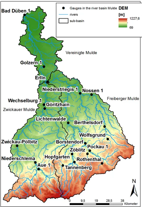
7.1.1. Mulde River Basin . . . 84

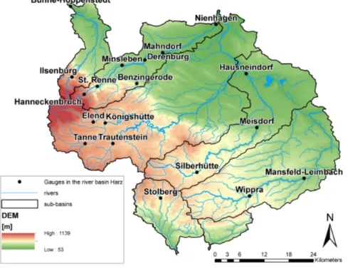
7.1.2. Harz Region . . . 87

7.2. Annualities and Design Floods . . . 87

7.2.1. How to estimate annualities . . . 89

7.2.2. Comparing robust estimators to non-robust ones in the hydrological context133 7.2.3. Application of robust estimators on the estimation of annualities . . . 144

7.3. Homogeneous Groups and Regionalisation . . . 162

7.3.1. A Regional Mixture Model . . . 169

7.4. Modelling Time Series . . . 175

8. Summary and Outlook 177

Bibliography 179

A. Appendix 191

2.1. AMS for the Wechselburg gauge and 99%-quantile . . . 7

2.2. Inuence of single events for AMS, POT and robust POT . . . 9

3.1. Monthly maximum and daily discharges of Wechselburg . . . 14

3.2. ACF of the monthly maximum and daily discharges of Wechselburg . . . 15

3.3. Daily discharges of Matapedia river . . . 20

3.4. ACF of daily discharges of Matapedia river . . . 21

3.5. Residuals and Engle-test for Matepedia . . . 21

3.6. QQ-plot of the residuals of Matapedia . . . 22

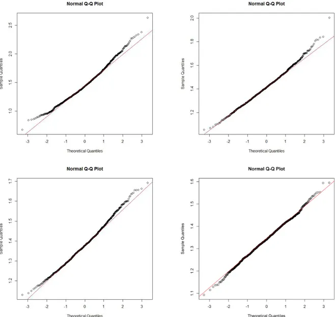
6.1. Normal QQ-plots for Gini's mean dierence under NED . . . 76

6.2. Normal QQ-plots for theLM S_n-estimator under NED . . . 77

6.3. Normal QQ-plots for theQ-estimator under NED . . . 78

6.4. Normal QQ-plots for Gini's Mean dierence under strong dependence for NED . 79 6.5. Normal QQ-plots for theLM S_n-estimator under strong dependence for NED . . 80

6.6. Normal QQ-plots for theQ-estimator under strong dependence for NED . . . 81

7.1. The Mulde river basin . . . 85

7.2. The Harz region . . . 88

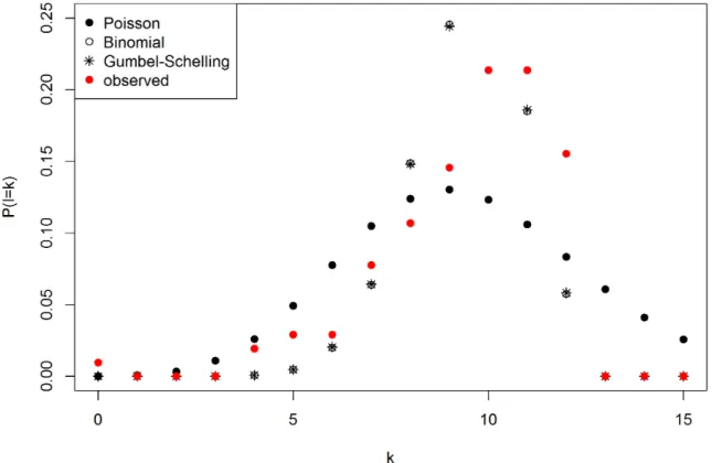
7.3. Dierences of discrete distributions for the number of exceedances . . . 93

7.4. Monthly means and maxima for two gauges in the Mulde river basin . . . 94

7.5. Burn-diagrams of TQ-values . . . 100

7.6. Peak-volume relationship and distinction into dierent ood types . . . 103

7.7. Peak-volume relationship and distinction into dierent ood types (three groups) 103 7.8. Boxplots for TQ-values of all ood types . . . 104

7.9. Dn in relation to the catchment size . . . 106

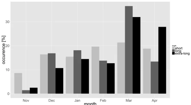
7.10. Distribution of ood types over the winter months . . . 107

7.11. The function f(ξ)of the mode of the GEV . . . 113

7.12. Relation of location and scale parameter of the GEV . . . 113

7.13. Share of the rst sample on the maximum series of two GEV-distributed samples 115 7.14. Normal QQ-plot of the non-overlaid part of a sample . . . 117

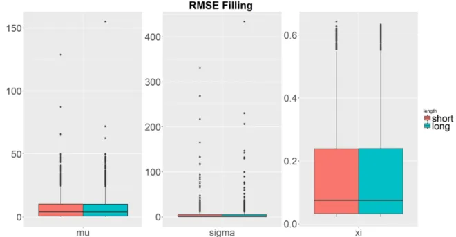
7.15. Boxplots for the RMSEs of the estimated parameters for long and short summer series using the lling method . . . 119

7.16. Boxplots for the RMSEs of the estimated parameters for long and short summer series using the lling method with share larger than 25% . . . 120

7.17. Boxplots of the estimates for the "lling method" under Scenario 3 . . . 124

7.18. Boxplots of the estimates for the "lling method" under Scenario 4 . . . 125

7.19. QQ-plot of lled series and the true sample . . . 126

7.20. Quantiles of the series of short and long summer annual maxima under use of the lling method or the non-overlaid subsamples for the gauge Berthelsdorf/Freiberger Mulde . . . 127

7.21. Short and long summer events with their estimated annuality and the tted mixing distributions . . . 128 7.22. Quantiles calculated for the Berthelsdorf/Freiberger Mulde gauge using dierent

statistical approaches . . . 129 7.23. Distribution functions of the series of short and long summer annual maxima at

the gauge Wechselburg/Zwickauer Mulde under use of the lling method or the subsamples . . . 129 7.24. Distribution functions calculated for the Wechselburg/Zwickauer Mulde gauge us-

ing dierent statistical approaches . . . 130 7.25. QQ-Plot of the annual maxima of the Berthelsdorf/Freiberger Mulde gauge com-

pared to the AMS, WS and WST model . . . 135 7.26. QQ-Plot of the annual maxima of the Wechselburg/Zwickauer Mulde gauge com-

pared to the AMS, WS and WST model. . . 136 7.27. QQ-Plot of the annual maxima of the Streckewalde/Preÿnitz gauge compared to

the AMS, WS and WST model . . . 137 7.28. Histogram of the estimated shape parameter for annual maxima of three river basins138 7.29. Fitting of the GEV (black) and Gumbel (grey) distribution to a GEV distribution

with increasing shape parameter viaL-moments . . . 142 7.30. Bias and RMSE of the Gumbel and GEV tting to i.i.d. GEV-distributed random

variables . . . 143 7.31. QQ-plot of pval for AMS, AMS (robust), POT and robust POT approaches . . . 146 7.32. QQ-plots for the annual maximum discharges of the Nossen gauge and the esti-

mates using AMS, robust AMS, POT and robust POT . . . 148 7.33. Empirical distribution ofSP AN_T . . . 149 7.34. Estimation of the99%-quantile of the Wechselburg and Nossen gauges for growing

sample length with four dierent approaches . . . 153 7.35. Coecient of variation of the 99%-quantile estimation for increasing sample length 154 7.36. Comparison of the AMS and the robust AMS, the POT and the robust POT by

the ratio between the ood quantiles . . . 155 7.37. Boxplots of all estimated99%-quantiles with the AMS or robust POT approaches

for year-by-year increasing sample length . . . 156 7.38. Comparison of the AMS, the POT and the robust POT approach by the estimated

99%-quantile for a year-by-year prolonged series . . . 158 7.39. Boxplot of the mean dierence of the last 100 estimates of a year-by-year prolonged

series calculated with the AMS and the robust POT approach . . . 159 7.40. Distribution functions calculated for the gauge Wechselburg using dierent robust

statistical approaches . . . 160 7.41. Estimation of the 99%-quantile of the Wechselburg gauge for growing sample

length with four dierent approaches . . . 161 7.42. QQ-plot of the AMS of the Wechselburg gauge compared with the robust AMS,

the robust WS and the robust WST model . . . 162 7.43. Estimation of the 99%-quantile of the simulated series for growing sample length

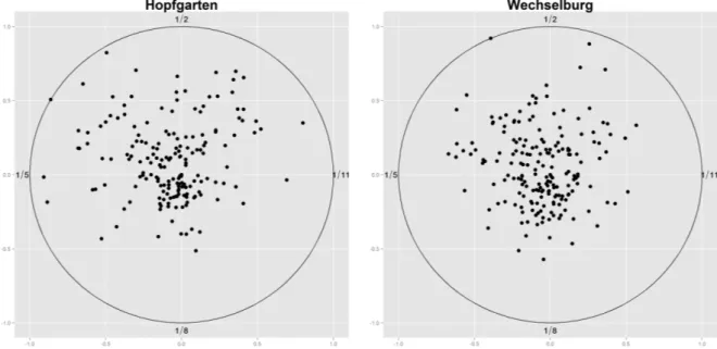
with four dierent approaches . . . 163 7.44. AMS, homogeneous and inhomogeneous classes of events for Hopfgarten and Licht-

enwalde . . . 170 7.45. Homogeneous and inhomogeneous classied events for Hopfgarten and Lichtenwalde171 7.46. Regional mixture model for the Lichtenwalde gauge . . . 173

7.47. Single components of the regional mixture model for the Lichtenwalde gauge . . . 174

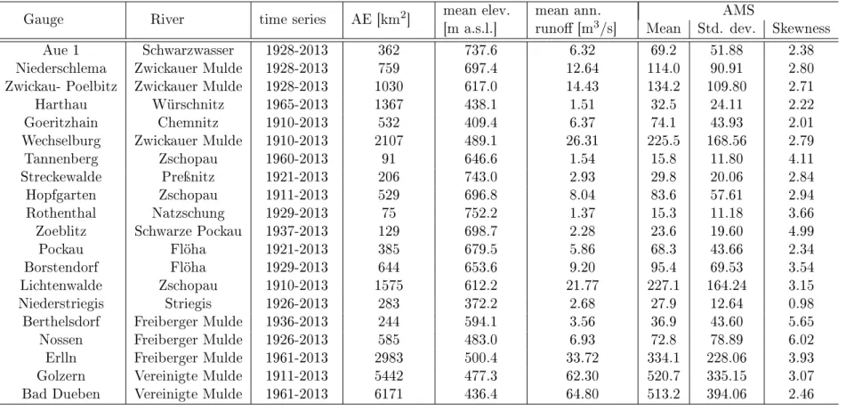
7.1. Parameters of the gauges in the Mulde river basin . . . 86 7.2. Annualities of the six largest annual maxima at the gauge Berthelsdorf/Freiberger

Mulde, estimated with both mixing approaches . . . 97 7.3. Statistical parameters for TQ-values . . . 101 7.4. Correlation between TQ and catchment area . . . 105 7.5. Mean and CV of ood timescales for dierent ood types and catchment sizes . . 108 7.6. RMSEs of the estimates of the GEV-parameters using Survival Analysis . . . 111 7.7. RMSEs of the estimates of the parameters using the lling method for sample

size n= 1000 . . . 121 7.8. RMSEs of the estimates of a GEV-sample for sample sizen= 1000 . . . 121 7.9. RMSEs of the estimates of the parameters using the lling method for sample

size n= 100 . . . 123 7.10. RMSEs of the estimates of the GEV-parameters using Survival Analysis . . . 123 7.11. Estimated parameters for the Berthelsdorf gauge with and without the method of

the lled series . . . 125 7.12. Estimated quantiles for the lled series and the maxima only. . . 126 7.13. Annualities at the Berthelsdorf/Freiberger Mulde gauge for the six largest oods

using three dierent models . . . 128 7.14. Estimated parameters of the GEV for the gauge Wechselburg/Zwickauer Mulde . 130 7.15. Annualities of the highest observed ood peaks at the Wechselburg/Zwickauer

Mulde gauge calculated with dierent statistical approaches . . . 130 7.16. Estimated annualities of the 2002 and 2013 events of the gauges in the Mulde

basin using AMS, WS and WST approach . . . 132 7.17. p-values of the Anderson-Darling test for a Goodness of Fit of the models GEV,

WS and WST . . . 134 7.18. Absolute dierences between predicted and observed return period of extraordi-

nary extreme oods for Wechselburg . . . 151 7.19. Absolute dierences between predicted and observed return period of extraordi-

nary extreme oods for Nossen . . . 151 7.20. Flood peaks with a return period of 100 years at Wechselburg and MAD from the

results of the total series with ve dierent approaches . . . 151 7.21. Flood peaks with a return period of 100 years at Nossen and MAD from the results

of the total series with four dierent approaches . . . 152 7.22. Estimated quantiles (in m³/s) for the Wechselburg gauge with the dierent models159 7.23. Possible classication of ood events with annualities . . . 165 A1. Goodness of Fit of the GEV, GPD, Gumbel (EVI) and Pearson III distribution to

the short and long summer maxima, the whole summer maxima and the winter and annual maxima with the Anderson-Darling test and the AIC . . . 192 A2. Share (in pct.) of the smallest values of a GEV(µ, σ, ξ) distributed sample that

can be removed without a signicant change of the estimated quantile . . . 193

A3. Estimation of the 99%- and the 99.9%-quantile for independent, identically Gum- bel (100, 10)-distributed random variables . . . 194 A4. Estimation of the 99%- and the 99.9%-quantile for independent, identically Gum-

bel (100, 10)-distributed random variables with extreme event . . . 195 A5. Estimation of the 99%- and the 99.9%-quantile for independent, identically GEV

(0.1, 100, 10)-distributed random variables . . . 196 A6. Estimation of the 99%- and the 99.9%-quantile for independent, identically GEV

(0.1, 100, 10)-distributed random variables with extreme events . . . 197 A7. Estimation of the 99%- and the 99.9%-quantile for independent, identically GEV

(0.2, 100, 10)-distributed random variables . . . 198 A8. Estimation of the 99%- and the 99.9%-quantile for independent, identically GEV

(0.2, 100, 10)-distributed random variables with extreme events . . . 199 A9. Classication of the gauges in the subcatchment Zwickauer Mulde/Chemnitz of

the Mulde river basin . . . 200 A10. Classication of the gauges in the subcatchment Freiberger Mulde/Flöha of the

Mulde river basin . . . 203 A11. Classication of the gauges in the Harz region . . . 206

A ood is dened as time-limited exceedance of discharge-thresholds in a cross-section of a river with a related drainage area caused by meteorological events (DIN 4049-1). This threshold is not dened precisely and depends on the local circumstances. For example, a ood can be dened as a discharge event that covers land that is typically not covered by water. In general, it is assumed that under humid conditions at least one ood occurs in a year (DWA (2012)).

Besides deterministic models (e.g. rainfall-runo models) statistical models and statistical evalu- ation are the most commonly used methods to describe the coherences of climatic, meteorological and discharge phenomena and to obtain predictions, for example for design events for ood pro- tection systems.

Since the processes leading to discharges can be explained by physical phenomena, it might seem somewhat articial to use stochastic models instead of deterministic ones. In fact, this is an often discussed and misunderstood point. The most important dierence between deterministic and stochastic models is the handling of errors (see e.g. Bierkens and van Geer (2008)). Stochastic models are developed to predict values at unknown time or at unknown location, where at the same time an assumption on the error can be made. That is, stochastic models give us the information how uncertain the estimation is. Errors in hydrological models can have many sources. First of all, not the real discharge is measured. Instead, often the water level at the gauge is measured and used to calculate the discharge by taking into account the ow velocity, that is a quantity based on empirical experiences. This of course causes uncertainty. Often even the assumptions on the stage-discharge relation change during the years and the discharge series of a gauge have to be calculated anew. Additionally, many of the main hydrological processes of runo formation leading to discharge cannot be observed since they proceed under the land surface. Groundwater or the permeability of the soil can just approximately be estimated based on information about the time of inltration or the soil conditions of the point scale. Most importantly, all models can only be seen as an approximation of the complex processes that lead to discharge. Even in deterministic hydrology these errors are taken into account. During the calibration the dierence to the residuals is minimized and the parameters are calculated.

After this step, though, the errors are no longer taken into account and, therefore, do not appear in the outcomes. In stochastic hydrology, the errors of the outcomes are handled as well. The treatment of discharge as random variable handles these errors indirectly. To make the dierence between the two approaches clearer we want to give an example following Bierkens and van Geer (2008). Consider the dischargex. Using a deterministic model this value is represented by the model outcomex^′. The made error can then be denoted byϵ=x^′−x, the so called residuum. In stochastic hydrology we now have additional information on the unknown error by considering it as random variable with known probability distribution. Often, not the error is treated as random variable but we assume the whole measurement x to be a random variable, the exact value of which we do not know, such that the error is treated indirectly.

Especially when considering extreme events, the use of stochastic models is advantageous com- pared to deterministic models, which typically underestimate extreme values. The rst explicit connections between statistical methods and hydrological data have been made in the 1940s

(Gumbel (1958)) when among others the mathematician Emil Julius Gumbel has investigated return periods of oods (Gumbel (1941)). Nevertheless, only descriptive statistic has been applied and no stochastic models have been widely used in hydrology until the 1970s, when the books of Vujica Yevjevich have been published (Yevjevich (1972a), Yevjevich (1972b)). Here, Yevje- vich tries to make the advantages of stochastic models and the complex information represented by them easier understandable and therefore better applicable by hydrologists by reducing the complexity to the cases relevant for hydrology and avoiding proofs. He explains the meaning of condence ranges and the importance of statistical tests and estimators besides multivariate con- sideration of hydrological data. Moreover, he is one of the rst hydrologists considering discharge series as time-variant process of stochastic nature, that can be autocorrelated or non-stationary.

This topic has been extended by Salas et al. (1980), where dierent kinds of dependence have been taken into account. This has then been the starting point of a wide use of stochastic mod- els and methods in hydrology and still today many newly developed concepts in statistics are applied in the hydrological context shortly after publication. A good example here are copulas.

Nevertheless, hydrological data also exhibit aspects that make statistical procedures more dicult to apply. The main problem when considering discharge series, especially maxima, is the limited period of observation. The construction of gauges and therefore the systematic conception of discharge data is in general not older than 100 years. Many gauges in Germany are in fact not observed for more than 30 years. Since the mostly considered ood series are annual maximum series, this results in sample lengths of about n = 30. Many statistical procedures based on asymptotic results fail here and many results are not valid for such small samples.

Additionally, we can nd many dierent types of dependence in the data series. Depending on the time-resolution, discharge series can exhibit long-range dependence (e.g. some daily discharge series), short-range dependence (e.g. daily and monthly discharge series) as well as independence (annual maximum series). Moreover, in many discharge series extraordinarily large events occur that have a large inuence on the estimation, especially in small samples. Also the dierent nature of the discharge series has to be taken into account. Whereas the annual as well as the monthly maximum series consist of ood peak measurements with the highest possible resolution, daily discharge series mostly consist of discharge means of a day. Additionally, anthropological and climatic changes (building of dams, heat periods) can lead to non-stationary behaviour, e.g.

heteroscedasticity. All these aspects have to be taken into account when using ood statistics.

In this thesis we place our focus on robust estimation methods in the context of ood statistics.

Robust estimation is expected to lead to more stable results that do not vary much over time.

That is, single extraordinary discharge events shall not have much inuence on the single esti- mations. Otherwise, the inuence of these events in short time series would be much too large.

Whereas the asymptotic distribution of robust estimators under independence is well known, few results exist under short-range dependence.

The rst part of this thesis therefore develops asymptotic normality as well as a long-run variance estimator under a form of short-range dependence for the class ofGL-statistics. These statistics cover many robust estimators, especially the linear as well as the trimmed linear moments, which are among the most commonly used estimators in hydrology. Hence, a concrete form of the limit distributions for these estimators is given. Since the theory is mainly based on the concept of U-statistics and U-processes, very general and in a broad statistical context applicable results are obtained. To take into account the heteroscedasticity of discharge data, we prove that the heteroscedastic model EGARCH exhibits the assumed concept of short-range dependence.

The results concerning robust estimation are then applied in the context of hydrology. Here, dierent concepts to estimate design oods are developed and their applicability is validated.

Moreover, a method to detect coherences between gauges in a river basin based on the classi- cation into alert steps is developed and applied to regionalisation where again the robustness of the estimators plays a crucial role.

The concept of robustness is used in many (statistical) disciplines, often with very dierent, sometimes even inconsistent, meaning. In general, there is no one-and-only valid denition for robustness and the use of this term often depends on the eld of application or even the author. Even in this work robustness has a mathematical as well as an application-oriented meaning. Whereas in statistics robustness can be clearly measured in certain ways, in hydrology (respectively almost all engineering disciplines) robustness is understood as a kind of stability, which is a very vague explanation. Of course, also statisticians want to obtain stability by using robust methods, nevertheless, the terms are dened much more specic. In the following, we will show that still both denitions are compatible and that statistically robust estimators lead to more stable estimations in the hydrological context. Some of the considerations made here can also be found in Fischer et al. (2015) and Fischer and Schumann (2016).

2.1. Denition

Following Huber (1981) we dene robustness as "insensitivity to small deviations from the as- sumptions". These deviations can be model misspecication or the wrong assumption on the convergence rate. In our context of hydrology and in general the most widely considered devia- tion is that of the shape of the underlying distribution respectively sample. Huber (1981) calls this "distributional robustness". Of course one could argue that this problem can be solved by simply removing outliers from the data, but in practice it becomes evident that it is not always clear, how to detect such outliers. Or it is not sensible to remove extreme values since they really occurred and are not erroneous data. This means they belong to the right tail of the underlying distribution but get too much weight in the estimation. Therefore, robustness is an important aspect when comparing estimators.

Now, even after giving the denition of robustness, there still exist many dierent aspects. For example Huber (1981) distinguishes between quantitative, qualitative or optimal robustness.

For more details on this topic and a more explicit description we refer to Huber (1981). The robustness measures described later on in this chapter focus on dierent aspects of robustness respectively.

2.2. Robustness in Hydrology

The estimation of ood quantiles with very low exceedance probabilities is a key problem of engineering hydrology. Since the number of recorded series of oods is very limited and seldom longer than 100 years, the needed probabilities of extreme ood events are derived from a tting of a suitable distribution function and its extrapolation into the realm of very low exceedance probabilities. The selection of the underlying statistical model is crucial in this context. There- fore, robustness is an important practical goal in ood statistics. It becomes evident when an extreme event with an exceedance probability signicantly smaller than1/noccurs within a time series of n years. Robustness in this context not only means robustness against extraordinary

extreme events but also against model misspecication or errors in the data. Whereas extraordi- nary extreme events are an important part of the ood series and contain important information this is not the case for data errors. This dierence has to be considered. Robust estimators therefore shall not be used to cut o these extreme events, but they shall be used to reduce the inuence of them especially in the presence of small sample lengths to gain stable estimates and to estimate the inuence of single extraordinary extreme events.

One problem consists of the temporal variability of statistical characteristics of these series, which results from exceptional extreme events happening occasionally. Those events have a large in- uence on the estimation of the parameters of the distribution functions and their quantiles temporarily. The impact of this temporal variability is aggravated if the demand for design oods is increasing after disastrous ood events, which often results in step changes of the es- timated parameters of distribution functions and of quantiles used as design criteria. In many cases, such changes are smoothed again by subsequent periods of normal oods. Figure 2.1 shows an example of step-wise changes of the 99 percent quantile derived from the general- ized extreme value (GEV) distribution with probability-weighted moments and a year-by-year extended ood series. If these quantiles are applied for the design of long-lasting hydraulic struc- tures, their temporal variability becomes a problem. There exist several approaches to handle such extraordinary events, causing step changes in hydrological parameters and quantiles. Often, these extraordinary events are treated as outliers and several statistical tests exist to detect such data points that deviate markedly from the remaining data points. By this, those values are treated like they are not drawn from the same population as the remainder data. For example, the Bulletin 17B, which is a benchmark in US-American hydrology, recommends such tests in a case of a skew larger than 0.4 (or smaller than −0.4 if we expect extraordinary low values) (Subcommittee (1981)). A very simple tool to dene outliers is the 3-σ-rule, which denes out- liers on the basis of the standard deviation (Jeong et al. (2017)). A well known test for these outliers is the maximum-value test of Grubbs (Grubbs (1969)). Here, it is assumed that the data follow approximately a normal distribution, but tests for the detection of outliers in data with other underlying distributions also exist (e.g. Spencer and McCuen (1996)). Also the tests by Dixon-Thompson, Rosner and Chauvenet are often recommended in the context of hydrology (see e.g. McCuen (2003)).

If an outlier is detected, still the question arises how to handle it. The outlier could be an erroneous value, which should be corrected or removed. Outliers in ood statistics may be the result of a mixed population occurrence (Kleme² (1986)). If we exclude these two possibilities, we can conclude that it is just an event from the tail of the distribution. Here we have two options: It could be censored to avoid distorting the analyses, or it could be weighted to reduce the resulting distortion.

The removal of conspicuous events has been the general handling of these values for a long time period (McCuen (2003)). Nevertheless, Gumbel already has remarked that "the rejection of outliers on a purely statistical basis is and remains a dangerous procedure. Its very existence may be a proof that the underlying population is, in reality, not what it was assumed to be"

(Kruskal et al. (1960)). During the last 30 years a change of the handling of extraordinary events has begun and several authors and even pamphlets of the federate states in Germany now recommend the consideration of these in the statistics (e.g. Ashkar (1993) and DWA (2012)). The option of weighting of such events became very popular by usingL-moments, which are rather robust to the eects of outliers (Hosking (1990)), or LH-moments (Wang (1997)), a generalization of L-moments, for characterizing the upper part of distributions and larger events in data.

There are other hydrological problems where a demand for robustness also exists, e.g. parameter

Figure 2.1.: Annual maximum discharges (HQ) for the Wechselburg/Zwickauer Mulde gauge in Saxony (1910-2013) and the estimated99%-quantile for increasing sample length. A jump in the estimated high quantile can be seen every time an extraordinary large event occurs, leading to an unstable estimation over the years.

calibration procedures for deterministic hydrological models (Guerrero et al. (2013)). Bárdossy and Singh (2008) have specied four criteria for an estimation of parameter vectors of such models in the framework of a data depth of observation periods. The parameter vectors should:

• lead to good model performance over the selected time period

• lead to a hydrologically reasonable representation

• not be sensitive against the choice of the calibration period

• be transferable to other time periods.

The third and fourth criteria are especially suitable for the interpretation of robustness used in this research. Since the estimated quantiles for certain annual return periods like T = 1000 are used for the design of long-lasting hydraulic structures, it is not desirable that these parameters change much with any extension of the observed time series. From the hydrological point of view a robust estimation is preferable that can mirror the asymptotic behaviour (limit) of the estimated quantile of the AMS to an early point of observation without having these step-changes.

In this context we want to focus on the interpretation of robustness as stability. That is, the estimation of extreme quantiles should not change signicantly when adding or removing only a few values. This intention shall be emphasised by an introducing example. The estimation methods presented here are not of interest in the moment and will be explained later on. Instead, we want to give an outline of the idea of robustness needed in hydrology. As shown in Figure 2.1, where the 99%-quantile for a year-by-year prolonged series of maximum discharges at the Wechselburg gauge is estimated, the inuence of single values on the estimation of high quantiles can be very large, especially when extraordinary large oods occur in very short time series. This instability leads to large problems if these quantiles are used as design oods. To emphasize the vulnerability of estimates of extreme quantiles in the presence of only a short period of observation we use a form of sensitivity curve to outline the inuence of single (extraordinary) oods.

For this we take the whole series of annual maxima (AMS) at the Wechselburg gauge(X1, . . . , Xn), remove the respective annual maximum for every time step and replace it by the median of the whole sample to gain a new sample X^′_i = (X₁, . . . , Xi−1,med(X₁, . . . , X_n), X_i+1, . . . , X_n) for i= 1, . . . , n. For these new samples a GEV or the Peak-over-threshold approach (POT) is tted using linear moments (L-moments) or trimmedL-moments (T L-moments) and the quantiles for the annualitiesT = 200,500,1000are calculated:

q_T;i =G⁻¹_X′ i

(T), where G⁻¹_X′

i is the quantile function of the GEV tted to the sample X^′_i. More details on the Peak-over-threshold approach as well as L-moments and T L-moments can be found later on in Sections 6.1.2 and 7.2.1. In this context they should only serve as examples of robust methods.

We nally take the dierence of qT;i and qT (the quantile based on the whole original sample) and multiply it with n+ 1. This is analogous to the classical sensitivity curve introduced in the next section, where instead of replacing one value by the median it is replaced by "one-wild"

(Tukey (1960)) to test the sensitivity of an estimator. Here, the "one-wild" observation is a real observation, whereas in statistical simulations often a function of a real-valued variable is used and the deviation for increasing values of this variable is measured. The use of the observations here should emphasise the problem of estimating a design ood, instead.

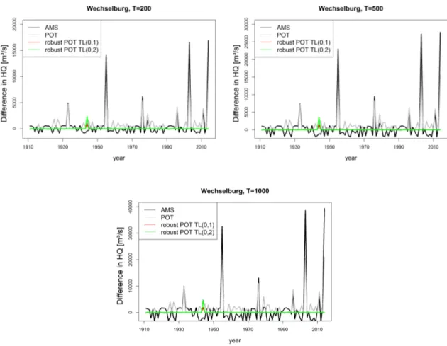
The results can be found in Figure 2.2, where the year displayed on the x-axis marks the year of the replaced observation.

Figure 2.2.: Inuence of single annual maxima on the estimation of the quantile with annuality T for dierent estimators and models by calculating the dierence to the quantiles based on the series without this annual maximum (sensitivity). For the non-robust estimators in AMS and POT-model the estimation is inuenced a lot by single events.

When using robust estimators like theT L-moments the inuence of this single events is reduced to almost zero leading to a stable estimation.

It becomes obvious that the extraordinary oods in the years 1954, 2002, and 2013 have a very high inuence on the estimation of the quantiles when using classical estimators like the L-moments. This inuence increases with increasing annuality. Therefore, the use of such quantile estimators in the design of dams can lead to serious problems since it is highly unstable.

Robust estimation approaches like the robust POT reduce this instability and are a noteworthy alternative. Additionally, they can be used to estimate the inuence of single events.

Although especially extreme events are of interest in hydrology, since they are the ones causing highest damage, the considerations made above show that also the use of robust estimators in hydrology is of considerable interest.

Additionally, it is not always clear, which kind of distribution function one should use, two- or three-parametric. Whereas the three-parametric distribution function allows a greater exibility in modelling the tails it is also more uncertain, especially when estimating the shape parameter.

Recommendations are for example given by the DWA (DWA (2012)), recommending a two- parametric distribution function for samples with less than 30 years and a three-parametric one for samples with more than 50 years. A distinct recommendation for samples of 30-50 years is not given. A robust estimator used in the hydrological context should therefore be also insensitive against small deviations from the model. Moreover, besides the GEV distribution there exist a lot of other distributions used in hydrology to model oods, for example the PearsonIII-distribution or the Gamma-distribution. Nevertheless, in the context of our considered data samples the GEV distribution is the most commonly used. More details on this context can be found in Section 7.2.1.

All these aspects play a crucial role in ood statistics and should have inuence on the used methods and estimators. Robustness could lead to an improvement of the consideration of uncertainty in this point.

2.3. Measures of Robustness

There exist several possibilities to measure robustness. All of them focus on dierent aspects of the denition made above. Additionally, some of the measures have been developed because of the special challenges in their eld of application. We want to dene two of the most common statistical measures of robustness as well as one measure that has its origin in hydrology, focussing especially on the right tail. All of them will be used later on to emphasise the robustness of certain models or estimators.

2.3.1. Inuence Curve

As mentioned above, one important aspect of robustness is the insensitivity of the estimation against single (extreme) values. This aspect somehow coincides with the hydrological point of view concerning stability: we do not want to obtain large deviations in the estimation if one extraordinary event occurs. The limit of the inuence of a single observation x on an estimate T(F_n) of F (just think about random variable X with distribution function F and a sample x1, . . . , xn with empirical distribution functionFn) can be expressed by (see Hampel (1971))

IC(x;F, T) = lim

λ→0

T((1−λ)F+λδx)−T(F)

λ ,

where δx denotes the point mass 1 at x. This is the so called inuence curve, which can be shown to have several interesting properties (see Section 5). In fact it is the rst derivative of

the estimator T evaluated at the perturbation of F by δ_x. For a robust estimator we of course want to have a bounded inuence curve indicating that also the inuence of single observations on the estimate is bounded.

Example 2.1. Assume we have i.i.d random variablesX1, . . . , Xn. The sample mean Xˆ =µ(Fn) =

∫ ∞

−∞

xdFn(x) = 1 n

n

∑

i=1

Xi

is an estimator for the expected valueµ(f) =∫∞

−∞xdF(x). It has inuence function IC(x;F, µ) = lim

λ→0

µ((1−λ)F+λδx)−µ(F) λ

= d dλ

∫ ∞

−∞

zd[(1−λ)F+λδx]|_λ=0= d

dλ((1−λ)µ(F) +λx)|_λ=0

=x−µ(F),

which increases unboundedly with increasingx. Thus, the sample mean is not robust.

There also exist several sample versions of the inuence curve, where we want to focus on the one proposed by Tukey (1960), the so-called sensitivity curve

SCn−1(x) = T(ⁿ⁻¹_n Fn−1+_n¹δ_x)−T(Fn−1)

1 n

,

where we simply replacedF by Fn−1 and λby _n¹. 2.3.2. Breakdown Point

Often, not only one extreme value occurs and in this case the knowledge of the inuence of a single value is not helpful. Here, we are interested in the behaviour of the estimate under the occurrence of many extreme values. The asymptotic breakdown pointϵ^∗of an estimatorT(Fn) of the functionalT(F)is dened as

ϵ^∗(T, F, d) = sup

ϵ<1

{ϵ: sup

F:d(F,F0)<ϵ

|T(F)−T(F0)|<∞}.

It characterises the maximum deviation from the true F₀ for a chosen metric d. For a nite sampleΩ =X1, . . . , Xn the sample breakdown point is then dened as

ϵ^∗_n(T) = 1 nmax

{

m: sup

Ωm

∥T(Ω_m)∥<∞ }

,

whereΩ_m is a sample derived fromΩ by replacing anymvalues ofΩ with arbitrary ones;

It gives us information on how many outliers can occur until the estimator collapses. A breakdown point of 0 indicates a totally non-robust estimator, whereas equivariant robust estimators can reach a breakdown point of50%. For example, the sample mean has breakdown point0, whereas the median has breakdown point0.5.

2.3.3. Stability Index

The breakdown point or the inuence or sensitivity curve are the most frequently used measures for robustness. However, these measures do not consider the special properties of hydrological data. When using ood series, the quantity of available data is very limited, and the asymptotic behaviour of the mathematical procedures are not eective. The special form of the applied mod- els, in which the estimated parameters have an exponential inuence on the resulting quantile, leads to large deviations in the results, even if the dierences between parameter estimations are small. Therefore, it is not sucient to check only the parameter estimators for their robustness, but the applied statistical model as a whole plays a crucial role. Hence, we use hydrologi- cal measures of stability of quantiles. Typical of most hydrological assessments of stability is the comparison of dierent calibration (in our case: modelling) and validation subperiods (cf.

Brigode et al. (2013)). For stability of quantiles, the criterionSP AN_T measuring the variability (span) of the estimation is used, which has been proposed by Garavaglia et al. (2011) and applied to compare the robustness of tting methods (Kochanek et al. (2014), Renard et al. (2013)).

The value ofSP AN_T for a quantile of the annual return period T at a given site l is calculated by

SPANT(l) =

1≤s≤bmax {ˆq_T;l(s)} − min

1≤s≤b{qˆ_T;l(s)}

1 b

b

∑

s=1

ˆ q_T;l(s)

,

whereqˆT;l(s)is the estimated quantile related to the return periodT for one ofbnon-overlapping subperiods s = 1, . . . , b at the gauge l. The optimal value of SP AN_T, indicating a robust, stationary behaviour of the statistical model, is 0. To compare the SP AN_T for several gauges at the same time, the empirical distribution can be considered for all l. Since in our case the sample length is very limited and the robust estimators need a certain quantity of data, we have to reduce the quantity of subperiods to two, choosing one with a length of 50 years. The SP ANT criterion can also be applied to compare quantiles of two parts of a time series s1 and s₂ as follows (Renard et al. (2013))

SP AN_T(l) = |ˆq_T;l(s₁)−qˆ_T;l(s₂)|

1

2(ˆq_T;l(s1) + ˆq_T;l(s2)),

where qˆ_T(si), i = 1,2, is the estimated quantiles related to the annual return period T for subperiods s₁ ands₂ respectively at the gaugel.

In contrast to the two above-mentioned measures, which are well-known in statistical theory, the SP AN-criterion is mainly used in the hydrological context. This is not only due to the fact that it measures the stability instead of the inuence of one value, but also because we can lay the focus on high quantiles by choosing appropriateT. Because of the comparison of two subsamples it is also possible to compare the inuence of two or more values on the estimation. Having in mind the often frequent appearing extraordinary events in hydrology, this is a desirable property.

By using the representation by the distribution ofSP AN of several gauges it is also possible to detect salience of single gauges. Hence, this measure will be used here especially in the context of hydrological ood series to take into account their special nature. Nevertheless, it is comparable to other statistical measures for robustness.

For several years, the concept of independent and identically distributed data has been the common assumption in hydrological statistics. And not only in hydrology, but also in many other applications independence has been assumed. Nevertheless, it is questionable whether discharge series, especially of high time-resolution, are really independent. As an example we take the monthly maximum discharges at the Wechselburg gauge in Germany, see Figure 3.1.

The Wechselburg gauge at the river Zwickauer Mulde belongs to the Mulde river basin located in Saxony in South-East Germany. The time series may look independent, but the autocorrelation function shows a dierent picture (Figure 3.2). We can see a signicant deviation from the condence bands based on White Noise and therefore from independence. Thus, one can assume a certain dependence in the data. Please note that both discharge series are not related directly, since the maximum values are peak measurements.

If one accepts the presence of dependence in the data, the question arises, which kind of depen- dence is present.

On the left hand side of Figure 3.2 one can see a fast decay of the autocorrelation function, whereas on the right hand side there is only a slow decay. Nevertheless, the same gauge is considered, only the type of discharges (monthly maxima and daily means) is dierent.

In general, most of the considered ood series in hydrology can be assumed to be independent or short-range dependent. Moreover, to detect long-range dependent behaviour, the time series considered here are not long enough. In the following we will therefore concentrate on the concept of short-range dependence.

There exist several denitions of dierent forms of short-range dependence. One of the most common ways to dene short-range dependence is by mixing processes.

Bradley (2007) gives an overview over the dierent forms of mixing. We will consider the case of absolutely regular sequences of random variables.

Denition 3.1. Let A,B ⊂ F be two σ-elds on the probability space (Ω,F,P). The absolute regularity coecient ofA andB is given by

β(A,B) =Esup

A∈A

|P(A|B)−P(A)|.

If (Xn)n∈N is a stationary process, then the absolute regularity coecients of (Xn)n∈N are given by

β(l) = sup

n∈N

β(F₁ⁿ,F_n+l^∞ ).

(X_n)n∈N is called absolutely regular, if β(l)→0 as l→ ∞.

Absolutely regular random variables are sometimes also calledβ-mixing and have been introduced by Volkonskii and Rozanov (1959). β-mixing is a stronger assumption than for exampleα-mixing, since for theα-mixing coecientsα given by

α(l) = sup

n∈N

sup{

|P(A∩B)−P(A)P(B)|:A∈ F₁ⁿ, B∈ F_n+l^∞ } ,

Figure 3.1.: Monthly maximum discharges (top) and daily means (bottom) of the Wechsel- burg/Zwickauer Mulde gauge. The dierence between the peak values and means becomes evident.

higher time-resolution show a much stronger dependence.

it holds that α(l) ≤ ¹₂β(l), so that every absolutely regular process is likewise strong mixing.

Though,β-mixing is weaker than Ψ- or Φ-mixing.

Typical examples for such absolutely regular processes are certain Markov chains or certain AR- processes. Nevertheless, more complex models like dynamical systems cannot be modelled by this concept of short-range dependence. For example Andrews (1984) has shown that even anAR(1) process of independent Bernoulli innovations is no longer α-mixing since one can construct sets that are determined by the future process, no matter how far away. Gorodetskii (1978) even has been able to show that there exist linear processes with normal distributed innovations, whose coecients decline too slowly, such that they are no longer mixing.

To cover all these processes, the so called near epoch dependence has been developed. It is based on the idea that although a random variableXt=f(. . . , Zt−1, Zt, Zt+1, . . .), which is a functional of a mixing sequence, is not necessarily mixing it depends on the near epoch of Z_t. Therefore, some properties can be concluded, especially the validity of limit theorems.

Denition 3.2 (Near Epoch Dependence (NED)).

Let ((X_n, Z_n))n∈Z be a stationary process. (X_n)n∈N is calledL₁ near epoch dependent (NED) on the process (Zn)n∈Z with approximation constants (a_l)l∈N, if

E

⏐

⏐

⏐X₁−E (

X₁|G_−l^l )⏐

⏐

⏐≤a_l l= 0,1,2, . . . , where lim

l→∞al= 0 and G_−l^l is theσ-eld generated by Z−l, . . . , Zl.

Near epoch dependent processes are sometimes described with the term approximating function- als. One of the rst applications of such kind of short-range dependent processes can be found in Ibragimov (1962). In the literature one often also nds L₂ or in general L_p near epoch de- pendence, where the L₁ norm is simply changed to theL_p norm, or the weaker form ofP-NED (Dehling et al. (2016); Vogel and Wendler (2015)), which allows to consider processes with exist- ing moments of lower order. The main dierence between the dierent denitions of near epoch dependence are their assumptions on the existing moments.

The concept of near epoch dependence is especially useful in the case of an underlying mixing sequence, since in this case very helpful properties are inherited. More details on this and a detailed introduction to near epoch dependence can be found in Davidson (2002).

For the two examples given above and also given in Andrews (1984) and Gorodetskii (1978) Jenish and Prucha (2012) show that they are near epoch dependent.

3.1. Examples

A typical example of a model for short-range dependent data is a special case of the ARIMA(p,d,q)- model, which is an abbreviation for Auto-Regressive Integrated Moving Average. As indicated by the name it consists of an AR-part of orderp as well as an MA-part of orderq.

Denition 3.3. A process (X_t)t∈Z is called ARIMA(p,d,q)-process if Xt=φ⁻¹(B)θ(B)(1−B)^−dZt,

where (Zt)t∈Z is a White Noise series anddis an integer. The polynomials φ(z) = 1−φ₁z−. . .−φ_pz^p

θ(z) = 1 +θ₁z+. . .+θ_qz^q

have no common zeros and φ has no roots on the unit circle. The operator B is the so-called Backshift Operator dened byBZt=Zt−1.

The parameter d is the integration parameter. It gives the times of dierentiation needed to obtain a stationary time series.

A stationary ARIMA-series, that isd= 0, is strongly mixing.

Some of the widely used models when considering near epoch dependent processes are GARCH- processes (Generalized Autoregressive Conditional Heteroscedasticity) (Bollerslev (1986)), a gen- eralisation of ARCH-processes. They are a common model for volatility clustering in nancial data and are also used for example in hydrology (Wang et al. (2012)).

Denition 3.4. A process(X_t)t∈Z is called GARCH(p,q)-process, if X_t=σ_tZ_t,

whereσ²_t is the positive conditional variance given by

σ_t²=α₀+α₁Z_t−1² +. . .+α_pZ_t−p² +β₁σ²_t−1+. . .+β_qσ²_t−q,

whereα0, . . . , αp, β1, . . . , βq∈Rare non-negative withαp̸= 0 andβq ̸= 0and(Zt)t∈Z is an i.i.d.

sequence with mean zero and variance equal to one.

Hansen (1991) relaxes the assumptions on (Z_t)t∈Z, such that (Z_t)t∈Z can be assumed to be α- mixing. He showed then that if(

E[(β1+α1(^X_σ^t

t)²)^r|F_t−1] )1/5

≤c <1a.s. for allt, a GARCH(1,1)- processX_tisL_r-NED on theα-mixing processZ_twith approximation constantsa_l=c^l2α₀c/(1−

c)and F_t=σ(. . . , Z_t).

An extension of the GARCH-model is the exponential GARCH (EGARCH) model proposed by Nelson (1991).

Denition 3.5. The process(Xt)t∈Z is called EGARCH(p,q)-process on the sequence (Zt)t∈Z, if Xt=σtZt,

whereσ²_t is the positive conditional variance given by

log(σ²_t) =α0+α1f(Zt−1) +. . .+αpf(Zt−p) +β1log(σ²_t−1) +. . .+βqlog(σ_t−q² ),

where α0, . . . , αp, β1, . . . , βq ∈R with αp ̸= 0 and βq ̸= 0 and f is a measurable function which is linear in Z and given by

f(Zt) =θZt+λ(|Z_t| −E|Z_t|) with parameters θ, λ∈R.

The termλ(|Z_t| −E|Z_t|)determines the size eect whereas θZ_tdetermines the sign eect of the shocks on volatility. It can be seen thatE(f(Z_t)) = 0.

One of the advantages of EGARCH-processes is that they do not have the non-negativity re- striction of the GARCH-processes. We show that under similar assumptions as for the GARCH- process an EGARCH-process is near epoch dependent.

Theorem 3.1. Let σ₁ be bounded and ∑q

i=1|β_i|<1. Moreover, assume that sup

t∈Z

E|Z_t|<∞. (3.1)

Then the EGARCH(p,q)-process on the sequence (Zt)t∈Z given by Xt = σtZt is near epoch dependent.

Remark 3.1. 1. The assumption (3.1) in Theorem 3.1 is an analogue to the condition of Hansen (1991) for GARCH-processes to the EGARCH-case with arbitrary valuespand q. Whether this condition is fullled depends on the existing moments ofZi. For example, if (Zt)t∈Z is a White Noise process with variance σ (that isE|Z_t| ≤σ = 1), the condition is fullled.

2. The boundedness of the conditional variance σ1 is a common assumption for GARCH- processes (see Hansen (1991), Lee and Hansen (1994)). It results from the moment con- dition on σ, E|σ₁|^1+δ < ∞, which is needed in the following proof, and the Lipschitz- condition.

Proof. (Theorem 3.1)

Using an iterative expression of the termlog(σ_t²) we obtain log(σ_t²) =

n

∑

j=1

∑

k1,...,kq∈N0, k1+...+kq=j−1

( j−1 k1, . . . , kq

)

β₁^k1 ·. . .·βq^kq

( α0+

p

∑

k=1

αkf (

Z_t−k−(^∑qi=1iki) )

)

+ ∑

k1,...,kq∈N0, k1+...+kq=n

( n k1, . . . , kq

)

β₁^k1 ·. . .·βq^kqlog(

σ_t−² (^∑qi=1iki) )

.

Now, considering the limit forn→ ∞, it is log(σ_t²)

= lim

n→∞

n

∑

j=1

∑

k1,...,kq∈N0, k1+...+kq=j−1

( j−1 k1, . . . , kq

)

β₁^k1·. . .·β_q^kq (

α₀+

p

∑

k=1

α_kf(

Z_t−k−(^∑qi=1iki) )

)

+ lim

n→∞

∑

k1,...,kq∈N0, k1+...+kq=n

( n k₁, ..., k_q

)

β₁^k1·. . .·βq^kqlog(

σ_t−² (^∑qi=1iki) )

.

We want to show that the rst term of the sum converges a.s. This is gained by the assumptions sup

t E|Z_t| < ∞ and |∑q

i=1βi| < 1 and the linearity of the function f. With the Multinomial Theorem and the convergence of the geometric series we can apply the monotone convergence theorem to obtain the convergence of the series (see for example Proposition 3.1.1 of Brockwell and Davis (2006)).

For the second term we show that it converges to zero a.s., that is

n→∞lim

∑

k1,...,kq∈N0, k1+...+kq=n

( n k1, . . . , kq

)

β₁^k1 ·. . .·β_q^kqlog( σ_t−²

(^∑qi=1iki) )

= 0 for all t∈Za.s.

By using the Multinomial Theorem we have

n→∞lim

∑

k1,...,kq∈N0, k1+...+kq=n

( n k1, . . . , kq

)

β₁^k1 ·. . .·βq^kqlog (

σ_t−² (^∑qi=1iki) )

≤ sup

k1,...,kq

log( σ_t−²

(^∑qi=1iki) )

n→∞lim

∑

k1,...,kq∈N0, k1+...+kq=n

( n k1, . . . , kq

)

|β₁|^k1·. . .· |β_q|^kq

= sup

k1,...,kq

log(

σ_t−² (^∑qi=1iki) )

n→∞lim(|β₁|+...+|β_q|)ⁿ and therefore the term converges a.s. to zero if

q

∑

i=1

|β_i|<1.

Hence, we can write log(σ²_t) =

∞

∑

j=1

∑

k1,...,kq∈N0, k1+...+kq=j−1

( j−1 k1, ..., kq

)

β₁^k1·...·β_q^kq (

α₀+

p

∑

k=1

α_kf(

Z_t−k−(^∑qi=1iki) )

) .

This is a linear solution and for this reason the process (log(σ_t²))t∈Z is near epoch dependent.

Moreover,

σt=

√

exp(log(σ_t²)) =g(log(σ_t²)) with g(x) = √

exp(x). This function g fulls the Lipschitz-condition for all x ∈ (−∞, a], a ∈ R. We can now apply Proposition 2.11 of Borovkova et al. (2001), where we need that σ1 is bounded. Therefore, the processσtand henceXt=σtZtis near epoch dependent on the process (Z_t)t∈Z.

3.2. Short-Range Dependence in Hydrology

Many time series in hydrology show a heteroscedastic behaviour. This can be caused by changing climate conditions but also by anthropogenic changes or other eects. More generally, almost all hydrological runo-models assume the residuals to be heteroscedastic. More precisely it is assumed that for small discharges only small deviations in the simulation can occur, whereas for large discharges also large deviations can occur. Therefore, this behaviour can not fully be modelled by classical ARIMA-models. For example, Modarres and Ouarda (2013a) show that when using only an ARIMA-model for heteroscedastic data the residuals remain heteroscedastic.

Now there are two possible solutions for this problem. The rst one is the use of a Box-Cox or similar transformation before applying the ARIMA-model. On the other hand one can also apply a heteroscedastic model to the residuals and obtain for example an ARIMA-GARCH model. In hydrological time series it is often not sucient to use a Box-Cox transformation only (Modarres and Ouarda (2013b)). Additionally, often the use of a model to describe the behaviour of the residuals is preferable because of the possible use of additional information (Evin et al. (2013)).

Figure 3.3.: Daily discharges [m³/s] (left) and location of the considered gauge of the Matapedia river near Quebec, Canada (right).

Hence, a model is needed which takes into account this heteroscedasticity. In the considered case, the EGARCH-model proved to be superior to the other models (Modarres and Ouarda (2013a)).

We want to seize the data example of Modarres and Ouarda (2013a) and use it to apply the developed theory under short-range dependence later on. The observed data are daily discharges from a gauge of the Matapedia river near the basin Amqui in South-Eastern Canada with a catchment area of 558 km² (Figure 3.3).

The autocorrelation of this series shows signicant dependence within the data (Figure 3.4).

To the logarithmised data an ARIMA(13,1,4)-model is tted. The same order has also been chosen by Modarres and Ouarda (2013a) and to make the results comparable we adopt this parametrisation. The logarithmisation as well as the dierentiation withd= 1has been chosen to reduce the high persistence of the data.

When we have a look at the residuals of this model applied to the data we see a heteroscedastic behaviour (Figure 3.5). Therefore, Modarres and Ouarda (2013a) apply the Engle-test to test on autoregressive heteroscedastic behaviour (Engle (1982)). For all lags the p-value is almost zero and therefore a signicant heteroscedastic behaviour is found (Figure 3.5).

The results stay the same when a Box-Cox-transformation is applied to the data (logarithmic or original) before tting the ARIMA-model. Hence, a model is needed that can cope with this kind of behaviour. Modarres and Ouarda (2013a) try dierent kinds of heteroscedastic models (GARCH, Power Garch) but the EGARCH model covers the behaviour best. The parameters are chosen as p = 3 and q = 1 for the EGARCH-model. If we compare the observed residuals and the ones modelled by the EGARCH(3,1)-model in a QQ-plot we observe a very good t (Figure 3.6) and also the results of the applied Goodness of Fit test (Vlaar and Palm (1993)) conrm this.

This data example emphasizes the necessity of complex dependence models like the EGARCH model which are not covered by the classical theory of dependent random variables using mixing assumptions.

Figure 3.4.: Autocorrelationfunction (ACF) of the daily discharges [m³/s] of the considered gauge of the Matapedia river near Quebec. A strong dependence of the data can be seen.

Figure 3.5.: Residuals resulting from the tted ARIMA(13,1,4)-model (left) and p-values of the Engle-test (right) of the considered gauge of the Matapedia river near Quebec. This indicates a GARCH-behaviour remaining in the residuals.

Figure 3.6.: QQ-plot of the observed residuals from the ARIMA(13,1,4)-model and theoretical residuals modelled with the EGARCH(3,1)-model of the considered gauge of the Matapedia river near Quebec. The model ts well to the data.