A multi-year observation of nitrous oxide at the Boknis Eck Time Series Station in the Eckernförde Bay

(1)

Biogeosciences, 16, 4097–4111, 2019 https://doi.org/10.5194/bg-16-4097-2019

A multi-year observation of nitrous oxide at the Boknis Eck Time Series Station in the Eckernförde Bay

(southwestern Baltic Sea)

Xiao Ma¹, Sinikka T. Lennartz^1,a, and Hermann W. Bange¹

1GEOMAR Helmholtz Centre for Ocean Research Kiel, Düsternbrooker Weg 20, 24105 Kiel, Germany

anow at: ICBM, University of Oldenburg, Oldenburg, Germany Correspondence:Xiao Ma (mxiao@geomar.de)

Received: 30 April 2019 – Discussion started: 23 May 2019

Revised: 19 September 2019 – Accepted: 26 September 2019 – Published: 25 October 2019

Abstract. Nitrous oxide (N₂O) is a potent greenhouse gas, and it is involved in stratospheric ozone depletion. Its oceanic production is mainly influenced by dissolved nutrient and oxygen (O₂) concentrations in the water column. Here we ex- amined the seasonal and annual variations in dissolved N₂O at the Boknis Eck (BE) Time Series Station located in Eck- ernförde Bay (southwestern Baltic Sea). Monthly measurements of N2O started in July 2005. We found a pronounced seasonal pattern for N2O with high concentrations (supersat- urations) in winter and early spring and low concentrations (undersaturations) in autumn when hypoxic or anoxic conditions prevail. Unusually low N₂O concentrations were observed during October 2016–April 2017, which was presumably a result of prolonged anoxia and the subsequent nutrient deficiency. Unusually high N₂O concentrations were found in November 2017 and this event was linked to the occurrence of upwelling which interrupted N₂O consumption via denitrification and potentially promoted ammonium oxidation (nitrification) at the oxic–anoxic interface. Nutrient concentrations (such as nitrate, nitrite and phosphate) at BE have been decreasing since the 1980s, but oxygen concentrations in the water column are still decreasing. Our results indicate a close coupling of N2O anomalies to O2concentration, nutrients, and stratification. Given the long-term trends of declining nutrient and oxygen concentrations at BE, a decrease in N2O concentration, and thus emissions, seems likely due to an increasing number of events with low N₂O concentrations.

1 Introduction

Long-term observation with regular measurement intervals can be an effective way to monitor seasonal and inter-annual variabilities as well as to decipher short- and long-term trends of an ecosystem, which are required to make projections of the future ecosystem development (e.g. see Ducklow et al., 2009). Recently, multi-year time series measurements of nitrous oxide (N₂O), a potent greenhouse gas and a major threat to ozone depletion (IPCC, 2013; Ravishankara et al., 2009), have been reported from the coastal upwelling areas off central Chile (Farías et al., 2015), off Goa (Naqvi et al., 2010), in the North Pacific Subtropical Gyre (Wilson et al., 2017), and in Saanich Inlet (Capelle et al., 2018).

N₂O production in the ocean is generally dominated by microbial nitrification (NH⁺₄ →NO⁻₂ →NO⁻₃) and denitrification (NO⁻₃ →NO⁻₂ →N₂O→N₂). During bacterial or archaeal nitrification, N2O is produced as a by-product with enhanced N2O production under low-oxygen (O2) conditions (e.g. Goreau et al., 1980; Löscher et al., 2012). N2O is produced as an intermediate during bacterial denitrification (Codispoti et al., 2005). N2O could be further consumed via denitrification to dinitrogen; however, this process is inhibited with the presence of O₂because of the low O₂tolerance of the enzyme involved (Bonin et al., 1989). This incomplete pathway is called partial denitrification and can lead to N₂O accumulation (e.g. Naqvi et al., 2000; Farías et al., 2009).

The oceans including coastal areas contribute∼25 % of the natural and anthropogenic N₂O emissions (IPCC, 2013), with disproportionately high emissions from coastal and estuarine areas (Bange, 2006). N₂O emissions from coastal

(2)

areas strongly depend on nitrogen inputs (Seitzinger and Kroeze, 1998; Zhang et al., 2010). The increasing input of nitrogen (i.e. eutrophication) has become a worldwide problem in coastal waters leading to enhanced productivity and severe O₂depletion caused by enhanced degradation of organic matter (Breitburg et al., 2018; Rabalais et al., 2014). The decline in O₂ concentration (i.e. deoxygenation), either in coastal waters or the open ocean, might result in favourable conditions for N₂O production (Codispoti et al., 2001; Nevi- son et al., 2003). The results of a model study by Kroeze and Seitzinger (1998) indicated a significant increase in N₂O in European coastal waters for 2050. Moreover, it has been suggested that N2O production and emissions are very likely to increase in the near future, especially in the shallow suboxic or anoxic coastal systems (Naqvi et al., 2000; Bange, 2006). However, model projections show a net decrease in future global oceanic N₂O emission during the 21st century (Martinez-Rey et al., 2015; Landolfi et al., 2017; Battaglia and Joos, 2018).

The Baltic Sea is a nearly enclosed, marginal sea with a very limited access to the open ocean via the North Sea. The restricted water exchange with the North Sea and extensive human activities, such as agriculture, industrial production, and sewage discharge in the catchment area led to high inputs of nutrients to the Baltic Sea. As a result, the areas affected by anoxia have been expanding in the deep basins of the central Baltic Sea (Carstensen et al., 2014). In order to control this situation, the Helsinki Commission (HELCOM) was established in 1974 and a series of measures have been taken to prevent anthropogenic nutrient input into the Baltic Sea. Consequently, the nutrient inputs (by riverine loads, direct point sources, and, for nitrogen, atmospheric deposition) to the Baltic Sea are declining (HELCOM, 2018a). How- ever, the number of low-O₂(i.e. hypoxic or anoxic) events in coastal waters of the Baltic Sea is increasing and deoxygenation is still going on (Conley et al., 2011; Lennartz et al., 2014). The deoxygenation in the Baltic Sea can affect the production and consumption of N₂O. Our group has been monitoring dissolved N₂O concentrations at the Boknis Eck Time Series Station, located in Eckernförde Bay (southwestern Baltic Sea), for more than a decade. In this study, we present monthly measurements of N2O and biogeochemical parameters such as nutrients and O2from July 2005 to De- cember 2017. The major objectives of our study were: (1) to decipher the seasonal pattern of N2O distribution in the water column, (2) to identify short-term and long-term trends of the N₂O concentrations, (3) to explore the potential role of nutrients and O₂ for N₂O production and consumption, and (4) to quantify the sea-to-air N₂O flux density at the time series station.

2 Material and methods 2.1 Study site

Sampling at the Boknis Eck (BE) Time Series Station (https:

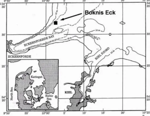
//www.bokniseck.de) started on 30 April 1957 and, therefore, it is one of the oldest continuously operated time series stations in the world. The BE station is located at the entrance of Eckernförde Bay (54^◦31⁰N, 10^◦02⁰E; Fig. 1) in the southwestern Baltic Sea. The water depth of the sampling site is 28 m. Various physical, chemical, and biological parameters are measured on a monthly basis (Lennartz et al., 2014). There is no significant river runoff to Eckern- förde Bay. Hence, the hydrographical conditions are mainly dominated by saline water input from the North Sea and less saline water from the Baltic Proper, which is typical for that region. Seasonal stratification usually starts to develop in April and lasts until October, during which hypoxia or even anoxia (characterized by the presence of hydrogen sul- fide, H₂S) sporadically occurs, as a result of restricted vertical water exchange and bacterial decomposition of organic matter in the bottom water (Hansen et al., 1999; Lennartz et al., 2014). Thus, BE is a natural laboratory to study the influence of O2variations and anthropogenic nutrient loads on N2O production and consumption.

2.2 Sample collection and measurement

Monthly sampling of N2O at the BE Time Series Station started in July 2005. Triplicate samples were collected from six depths (1, 5, 10, 15, 20, and 25 m). Seawater was drawn from 5 L Niskin bottles into 20 mL brown glass vials after overflow. The vials were sealed with rubber stoppers and alu- minium caps. The bubble-free samples were poisoned with 50 µL of a saturated mercury chloride (HgCl₂) solution and then stored in a cool, dark place until measurement. The general storage time before measurements of the N₂O concentrations was less than 3 months.

The static headspace equilibrium method was adopted to measure the dissolved N₂O concentrations in the vials.

A 10 mL helium (99.9999 %, AirLiquide, Düsseldorf, Ger- many) headspace was created in each vial with a gas-tight glass syringe (VICI Precision Sampling, Baton Rouge, LA, USA). Samples were vibrated with a vortex (G-560E, Sci- entific Industries Inc., NY, USA) for 20 s and then left for at least 2 h until equilibrium. A 9.5 mL subsample of the headspace was subsequently injected into a GC-ECD (gas chromatograph equipped with an electron capture detector) system (Hewlett-Packard 5890 Series II, Agilent Technolo- gies, Santa Clara, CA, USA), which was calibrated with two standard gas mixtures (N₂O in synthetic air, 320 and 1000 ppb, Deuste Steininger GmbH, Mühlhausen, Germany and Westfalen AG, Münster, Germany) prior to the measurement. The average precision of the measurements, calculated as the median standard deviation from triplicate measure-

(3)

X. Ma et al.: A multi-year observation of nitrous oxide 4099

Figure 1.Location of the Boknis Eck Time Series Station in the Eckernförde Bay, southwestern Baltic Sea. (Map from Hansen et al., 1999.)

ments, was 0.4 nM. Triplicates with a standard deviation of

> 10 % were omitted. More details about the N₂O measurement can be found in Kock et al. (2016). Dissolved oxygen (O2) concentrations were measured by Winkler titra- tions (Grasshoff et al., 1999). Nutrient concentrations were measured by segmented continuous-flow analysis (SCFA;

Grasshoff et al., 1999). A more detailed summary of the parameters measured and methods applied can be found in Lennartz et al. (2014).

2.3 Times series analysis

A time series can be decomposed into three main compo- nents, i.e. trend, cycle, and residual component (Schlittgen and Streitberg, 2001). We used the Mann–Kendall test and wavelet analysis to detect the trend and periodical cycles in the time series data, respectively. As for the residual component, we highlight unusual high or low N₂O concentrations during 2005–2017 and discuss the potential causes for these events.

2.3.1 Wavelet analysis

In order to decipher periodical cycles of the parameters collected at the BE Time Series Station, a wavelet analysis method was adopted. Wavelet analysis enables the detection of the period and the temporal occurrence of repeated cycles in time series data. One of the requirements for wavelet analysis is a regular, continuous time series. Since there are

data missing (maximum 2 months in a row) in the BE time series, due to terrible weather or the ship’s unavailability, missing data were interpolated from the previous and following months. Sampling time varied for every month (usually 20–40 d interval) but for the statistical analysis data were assumed to be regularly spaced as the uncertainty introduced was not significant (< 5 %). Considering the band width in both frequency and time domain, a Morlet mother wavelet with a wave number of 6 was chosen (Torrence and Compo, 1998). The mother wavelet was then scaled between the frequency of a half-year cycle and the length of the time series with a step size of 0.25. The wavelet analysis was conducted with the MATLAB code by Torrence and Compo (2004).

More information about the method can be found on the web- site http://paos.colorado.edu/research/wavelets/ (last access:

23 October 2019).

2.3.2 Mann–Kendall test

Mann–Kendall test (MKT) is a non-parametric statistical test to assess the significance of monotonic trends for time series measurements. It tests the null hypothesis that all variables are randomly distributed against the alternative hypothesis that a monotonic trend, either increase or decrease, ex- ists in the time series on a given significance levelα(here α=0.05). MKT is flexible for data with missing values and the results are not impacted by the magnitude of extreme values, which makes it a widely used test in hydrology and climatology (e.g. Xu et al., 2003; Yang et al., 2004). How-

(4)

ever, MKT is sensitive to serial correlation in the time series.

The presence of positive serial correlation would increase the probability of trend detection even though no such trend ex- ists (Kulkarni and von Storch, 1995). In order to avoid this situation, data from 12 months were tested individually. It is assumed that there is no residual effect left from the same month last year, considering that the nitrogen species are rapidly biologically cycled. The MATLAB function from Si- mone (2009) was used for the MKT.

2.4 Calculation of saturation and sea-to-air flux density N2O saturations (SN₂O, %) were calculated as

S_N₂_O =100×N₂O_obs/N₂O eq., (1) where N2Oobsand N2O eq.(nM) are the observed and equili- brated N2O concentrations in seawater, respectively. N2O eq.

was computed as a function of surface seawater temperature, in situ salinity (Weiss and Price, 1980), and the dry mole fractions of atmospheric N₂O at the time of the sampling. Since the atmospheric N₂O mole fractions were not measured at the BE Time Series Station, atmospheric dry mole fractions of N₂O were derived from the monthly average of N₂O data at Mace Head, Ireland, instead (AGAGE, Advanced Global Atmospheric Gases Experiment, http://agage.mit.edu/, last access: 23 October 2019).

N₂O flux density (F_N₂_O, µmol m⁻²d⁻¹) was calculated as FN₂O=kN₂O×(N2Oobs−N2O eq.) , (2) wherek_N₂_O (cm h⁻¹) is the gas transfer velocity calculated with the method given by Nightingale et al. (2000), as a function of the wind speed and the Schmidt number (Sc).

The wind speed data were obtained from Kiel lighthouse (see https://www.geomar.de/service/wetter/, last access: 23 Octo- ber 2019), which is approximately 20 km away from the BE Time Series Station. The wind speed was normalized to 10 m (u10) to calculatekN₂O(Hsu et al., 1994).kN₂Owas adjusted by multiplying with (Sc/600)^−0.5, andScwas computed as

Sc=v/D_N₂_O, (3)

D_N₂_O=3.16×10⁻⁶e^−18370/RT, (4) wherevis the kinematic viscosity of seawater, which is calculated from the empirical equations given in Siedler and Pe- ters (1986), andDN₂Ois the diffusion coefficient of N2O in seawater. R is the universal gas constant andT is the water temperature in kelvin.

3 Result and discussion 3.1 Overview

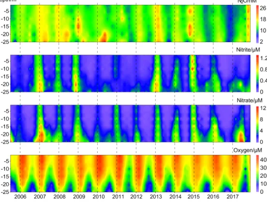
N₂O concentrations at the BE Time Series Station showed significant temporal and depth-dependent variations from

2005 to 2017 (Fig. 2). N2O concentrations fluctuated between 1.2 and 37.8 nM, with an overall average of 13.9± 4.2 nM. This value was higher than the results from the surface water of Station ALOHA (5.9–7.4 nmol kg⁻¹, average 6.5±0.3 nmol kg⁻¹; Wilson et al., 2017), which is reasonable considering the weak anthropogenic impact in the North Pa- cific Subtropical Gyre. The N₂O concentrations at BE were much lower than those measured at the time series station in the coastal upwelling area off Chile (2.9–492 nM, average 39.4±29.2 nM in the oxyclines and 37.6±23.3 nM in the bottom waters; Farías et al., 2015) and a quasi-time-series station off Goa (Naqvi et al., 2010), where significant N2O ac- cumulations are observed in subsurface waters at both loca- tions. Our measurements were comparable to the time series station from Saanich Inlet (∼0.5–37.4 nM, average 14.7 nM;

Capelle et al., 2018), a seasonally anoxic fjord which has similar hydrographic conditions as BE.

NO⁻₂ concentrations fluctuated between below the detection limit of 0.1 and 1.6 µM, with an average of 0.2±0.3 µM.

NO⁻₃ concentrations varied from below the detection limit of 0.3 to 17.9 µM, with an average of 2.0±2.8 µM. The temporal and spatial distributions of nitrite (NO⁻₂) and nitrate (NO⁻₃) were similar during 2005–2017. A clear O₂seasonality can be seen with severe O₂depletion in the bottom waters during summer and autumn. Anoxia with the presence of H₂S were detected in September and October 2005, Septem- ber 2007, September and October 2014, and September–

November 2016. All of the extremely low N2O concentrations (< 5 nM) were observed in the bottom waters in autumn, coinciding with hypoxia or anoxia, while the high N2O concentrations (> 20 nM) sporadically occurred at different depths either in spring or autumn.

3.2 Seasonal cycle

Significant cycles at different frequencies were detected via wavelet analysis at the BE Time Series Station during 2005–

2017 (Fig. 3). A half-year NO⁻₂ cycle sporadically occurred in 2007–2009, 2013, and 2015. There is a seasonal NO⁻₂ variability (at the frequency of 1 year) between 2007 and 2016 (times before 2007 and after 2016 were outside the conic line), except during 2010–2012, when high NO⁻₂ concentrations were not observed in winter (Fig. 2). A biennial cycle of NO⁻₂ could be observed as well during 2008–2015. The NO⁻₃ concentrations were dominated by an annual cycle and a mi- nor half-year cycle. The biennial cycle only occurred in 2008 and 2009. A remarkable seasonal variability in dissolved O₂ prevailed all the time, which is also obvious from the time series data shown in Fig. 2. The annual N₂O cycle became gradually more and more evident until 2014, then declined and reoccurred less intensely in 2016. The periodical cycle was also present at other frequencies, indicated by the broad- ening of the red area before 2015 in Fig. 2d. For example, a biennial N₂O cycle occurred during 2013–2015.

(5)

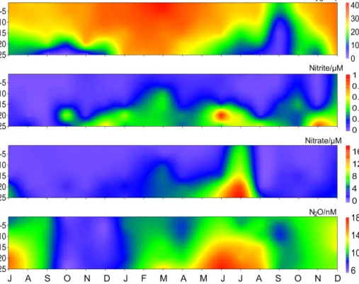
Figure 2.Vertical distributions of dissolved O₂, NO⁻₂, NO⁻₃, and N₂O from the BE Time Series Station during 2005–2017.

Figure 3.Wavelet power spectra of NO⁻₂ (a), NO⁻₃ (b), dissolved O₂(c), and N₂O(d)from the BE Time Series Station. Red areas indicate high power and blue areas indicate low power. The black conic line indicates the significant area where boundary effects can be excluded.

(6)

The half-year cycles of NO⁻₂ and NO⁻₃ were probably associated with algae blooms which usually occur in each spring and autumn (Figs. S1 and S2 in the Supplement).

Since the time between the two blooms differed between years, the cycles were weak and thus not present in every year. Due to the fact that there was no half-year O₂cycle at all, nutrients apart from O₂might be the “drivers” of the spo- radic half-year N₂O cycle in 2008 and 2015 because N₂O production depends on the concentration of the bioavailable nitrogen compounds (Codispoti et al., 2001).

Generally the wavelet analysis indicated a strong annual cycle for NO⁻₂, NO⁻₃, dissolved O2, and N2O at the BE Time Series Station, which enabled us to explore the seasonal pattern with annual mean data. Although extreme values were excluded as a result of averaging, the smoothed results generally reflect the seasonality of these parameters. Here, we focus on the annual cycle.

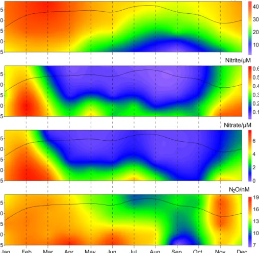
The annual mean vertical distribution of dissolved O₂, NO⁻₂, NO⁻₃, and N₂O are shown in Fig. 4. Due to the development of stratification, the mixed layer was shallow in summer and deep in late autumn and winter. O₂ depletion was observed in bottom waters from late spring until late autumn.

The seasonal variations in NO⁻₂ and NO⁻₃ were significantly correlated with each other ([NO⁻₃]=11.59[NO⁻₂]−0.51, R²=0.80,n=72,p<0.0001) and high concentrations were observed for both in winter. Minimum N₂O concentrations were found in the bottom waters during September and Oc- tober, presumably as a result of consumption during denitrification under anoxic condition (Codispoti et al., 2005). High N2O concentrations were observed in late spring and late autumn, respectively. In late spring N2O accumulated in the bottom waters because the stratification prevented mixing of the water column. In late autumn, however, N₂O could be ventilated to the surface and thus emitted to the atmosphere due to the breakdown of the stratification. The high N₂O concentrations could be attributed to enhanced N₂O production via nitrification and/or denitrification within the oxic–anoxic interface (Goreau et al., 1980; Codispoti et al., 1992). Since there is no clear O₂concentration threshold, N₂O production from both nitrification and the onset of denitrification overlap at oxic–anoxic interface. To this end, direct N₂O production measurements (i.e. nitrification and denitrification rates) are required to decipher which process dominates the formation of the different N2O maxima.

High N2O concentrations prevailed all over the water column in winter and early spring. NH⁺₄ is released from the sediment into bottom waters due to the degradation of organic matter, especially after the autumn algae bloom (Figs. S1 and S2 in the Supplement). The stratification usually completely breaks down at this time of the year and the water column becomes oxygenated. Denitrification is inhibited by the presence of high concentrations of dissolved O₂ (> 20 µmol L⁻¹, which is higher than the O₂ threshold of about 10 µmol L⁻¹; Tiedje, 1988) and thus nitrification is

presumably responsible for the high N2O concentrations in winter and early spring.

3.3 Trend analysis

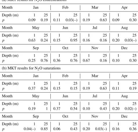
The MKTs were conducted for the surface (1 m) and bottom (25 m) N₂O concentrations and saturations of the individual 12 months, respectively. Significant decreasing trends were detected for the concentrations in the bottom waters for February and August (Table 1a), and for the saturations in the surface for September and in the bottom for August and November (Table 1b). These results indicated that some sys- tematical changes in N₂O took place at BE. For example, the significant decrease in N2O concentration/saturation in August might be associated with the increasing temperature, which reinforces the stratification and accelerates O2 consumption in the bottom waters (Lennartz et al., 2014). As a result, hypoxia/anoxia starts earlier and thus enables the onset of denitrification to consume N₂O. During most of the months, trends in N₂O concentration and saturation were not significant during 2005–2017.

A significant nutrient decline has been observed at the BE Time Series Station since the mid-1980s; however, Lennartz et al. (2014) found that bottom O₂concentrations were still decreasing over the past 60 years. The ongoing oxygen decline was attributed to the temperature-enhanced O₂ consumption in the bottom water (Meier et al., 2018) and a pro- longation of the stratification period at the BE Time Series Station (Lennartz et al., 2014). Please note that the trends in nutrients and O2 concentrations were detected based on the data collection, which lasted for approximately 30 and 60 years, respectively, while the N2O observations at BE Time Series Station have lasted for only 12.5 years. Fur- ther MKT analysis for nutrients, temperature, and oxygen for months with significant trends in N₂O concentrations did not show any significant results (p>0.05). The significant trends in N₂O concentrations thus do not seem to be directly related to one of these parameters, and we cannot state a reason for the significant trends of N₂O concentration in February and the N₂O saturation in September and November at this point.

Presumably, a longer monitoring period for N₂O is required to detect corresponding trends in N₂O and oxygen or nutrients.

3.4 Extreme events

3.4.1 Low N2O concentrations during October 2016–April 2017

Besides the low N₂O concentrations occurring in autumn, we observed a band of pronounced low N₂O concentrations which started in October 2016 and lasted until April 2017 (Fig. 5). In this period N₂O concentrations varied between 5.5 and 13.9 nM, with an average of 8.4±2.0 nM. This is approximately 40 % lower than the average N₂O concentration

(7)

Figure 4.Average vertical distributions of dissolved O₂, NO⁻₂, NO⁻₃, and N₂O from the BE Time Series Station during 2005–2017. The black line indicates the mixed layer depth, which was calculated based on a potential density anomaly of 0.15 kg m⁻³from the sea surface (1 m).

during the entire measurement period 2005–2017. The average N₂O saturation during 2005–2017 was 111±30 %, while from October 2016 to April 2017 the N₂O saturations were as low as 43 %–93 % (average 62±10 %).

Undersaturated N2O waters have been previously reported from the Baltic Sea: Rönner (1983) observed a N2O surface saturation of 79 % in the central Baltic Sea and attributed the undersaturation to upwelling of N2O-depleted waters. Bange et al. (1998) found a minimum N2O saturation of 91 % in the southern Baltic Sea where the hydrographic conditions were significantly influenced by riverine runoff. Walter et al. (2006) reported a mean N₂O saturation of 79±11 % for shallow stations (< 30 m) in the southwestern Baltic Sea in October 2003. The low-N₂O event at BE was unusual because the concentrations were much lower than those reported values and it lasted for more than half a year.

Although the observed temperatures and salinities during October 2016–April 2017 were comparable to other years (Fig. S1), it is difficult to evaluate the role of physical mech- anism in the low-N2O event because of insufficient data for water mass exchange at the BE Time Series Station.

Here we mainly focused on the chemical or biological processes. Anoxia events with the presence of H₂S were observed in the bottom waters for 3 months in a row during September–November 2016. This is an unusual long period and is unprecedented at the BE Time Series Station. In December 2016 the stratification did not completely break down. Although the water column was generally oxygenated, bottom O2 concentrations were the lowest observed during the past 12.5 years. Considering the classical view of N2O consumption via denitrification under hypoxic and anoxic conditions, we inferred that denitrification accounted for low N₂O concentrations in the bottom layer. However, the ques- tion of where the low N₂O concentration water in the upper layers came from still remains.

In September 2016, low N₂O concentrations were only observed in the bottom waters where the anoxia occurred.

However, the situation was different in the following months.

During October/November 2016, N₂O concentrations were homogeneously distributed in the water column. Although the stratification gradually started to break down in late autumn, the density gradient was still strong enough to keep

(8)

Table 1.The results of the Mann–Kendall test for the surface and bottom N₂O concentrations and saturations of the 12 individual months.

(a) MKT results for N₂O concentrations

Month Jan Feb Mar Apr

Depth (m) 1 25 1 25 1 25 1 25

p 0.09 0.19 0.11 0.03(–) 0.19 0.63 0.09 0.30

Month May Jun Jul Aug

Depth (m) 1 25 1 25 1 25 1 25

p 0.63 0.24 0.15 0.95 0.16 0.16 0.20 0.03(–)

Month Sep Oct Nov Dec

Depth (m) 1 25 1 25 1 25 1 25

p 0.25 0.76 0.36 0.76 0.67 0.16 0.10 0.30 (b) MKT results for N₂O saturations

Month Jan Feb Mar Apr

Depth (m) 1 25 1 25 1 25 1 25

p 0.37 0.24 0.15 0.15 0.19 0.63 0.11 0.19

Month May Jun Jul Aug

Depth (m) 1 25 1 25 1 25 1 25

p 0.19 1 0.37 0.54 0.10 0.43 0.20 0.02(–)

Month Sep Oct Nov Dec

Depth (m) 1 25 1 25 1 25 1 25

p 0.04(–) 0.85 0.06 0.43 0.20 0.03(–) 0.16 0.36

pindicates thepvalue of the test, which is the probability, under the null hypothesis, of obtaining a value of the test statistic as extreme or more extreme than the value computed from the sample. (–) indicates a rejection of the null hypothesis atαsignificance level and a decreasing trend is detected.

the bottom waters at anoxic conditions and prevented the low-N₂O-concentration water to reach the surface. Thus we inferred that the unusual low N₂O concentrations in the upper layers (above 20 m) were probably resulting from advec- tion of adjacent waters. Due to the fact that the upper layers were well-mixed and oxygenated, in situ N2O consumption in the water column could be neglected. We suggest, therefore, that the N2O-depleted waters were resulting from consumption of N₂O in bottom waters elsewhere and then they were upwelled and transported to BE. Hence, N₂O consumption via denitrification might have been, directly or indirectly, responsible for the low N₂O concentrations during October–

November 2016.

In December 2016, the bottom waters were ventilated with O₂. Although N₂O consumption by denitrification should have been inhibited by the high concentrations of O₂(Codis- poti et al., 2001), the N₂O concentrations did not restore to their normal level under suboxic conditions. Since Jan- uary 2017, the whole water column was well mixed and oxygenated. Usually a significant nutrient supply could be observed starting in November (Fig. 4) as a result of remineral- ization and vertical mixing, but the average NO⁻₂ and NO⁻₃ concentrations during November 2016–April 2017 were 0.2

and 1.4 µM, respectively, which was about 50 % and 60 % lower than in other years. Ammonium (NH⁺₄) and chloro- phyllaconcentrations during this period were comparable to those of other years (Fig. S1). Secchi depth, a proxy of water transparency, was 3.8 m in March 2017, which is only slightly lower compared to the monthly average value for March (4.5±1.8 m). There is no exceptional spring algae bloom and thus we infer that assimilative uptake of nutrients by phytoplankton was not responsible for the low nutrient concentrations. The nutrient deficiency might be attributed to enhanced nitrogen removal processes like denitrification or anammox (Voss et al., 2005; Hietanen et al., 2007; Hannig et al., 2007) during the prolonged period of anoxia in autumn 2016. During the low-N₂O event, we found that N₂O concentrations were positively correlated with both NO⁻₂ ([N₂O]=7.02[NO⁻₂]+7.36, R²=0.29, n=24, p<0.01) and NO⁻₃ ([N₂O]=0.80[NO⁻₃]+7.36, R²=0.51, n=24, p<0.0001). These results indicate that the development and maintenance of the low N2O concentration was closely associated with nutrient deficiency. Especially after the breakdown of the stratification, when denitrification was no longer a significant N2O sink, nutrients might have become a limit- ing factor for N2O production.

(9)

Figure 5.Vertical distribution of dissolved O₂, NO⁻₂, NO⁻₃, and N₂O from the BE Time Series Station during July 2016–December 2017.

Please note that the high N₂O concentrations in November 2017 were removed for better visualization.

In general, the low-N₂O-concentration event during Octo- ber 2016–April 2017 can be divided into two parts: in the stratified waters during October–November 2016, O₂played a dominant role and N₂O was consumed via denitrification under anoxic conditions. In the well-mixed water column during December 2016–April 2017, nutrient deficiency seemed to have constrained N₂O production via nitrification under suboxic/oxic conditions.

In recent years a novel biological N2O consumption pathway, called N2O fixation, which transforms N2O into partic- ulate organic nitrogen via its assimilation, has been reported (Farías et al., 2013). This process can take place under extreme environmental conditions even at very low N₂O concentrations. Cornejo et al. (2015) reported that N₂O fixation might play a major role in the coastal zone off central Chile where seasonally occurring surface N₂O undersaturation was observed. The relatively high N₂fixation rates in the Baltic Sea (Sohm et al., 2011) highlight the potential role of N₂O fixation (Farías et al., 2013). However, we cannot quantify the role of biological N₂O fixation for the N₂O depletion in the Baltic Sea due to the absence of N₂O assimilation measurements.

3.4.2 High N₂O concentrations in November 2017 High N₂O concentrations were observed at the BE Time Se- ries Station in November 2017. The average value reached 35.4±1.5 nM, which was the highest concentration measured

during the entire sampling period from 2005 to 2017. Dis- solved N₂O was homogeneously distributed in the water column, but this event did not last long. In December, dissolved N₂O returned to normal levels and the average concentration in the water column was comparable to that of other years.

Average N₂O saturation in November 2017 was 322±10 %, which was also the highest for the past 12.5 years. This value was much higher than the maximum surface N2O saturation reported by Rönner (1983) in the central Baltic Sea but was comparable to the results observed in the southern Baltic Sea (312 %; Bange et al., 1998). Bange et al. (1998) linked the enhanced N₂O concentrations to riverine runoff because those samples were collected in an estuarine area; however, the riverine influence around the BE Time Series Station is negligible. As a result, the impact of fresh water input can be excluded.

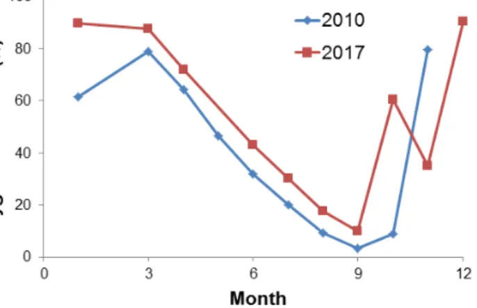
Dissolved O₂seemed to play a dominant role in the high N₂O concentrations. Enhanced N₂O production usually occurred at the oxic–anoxic interface, which was closely linked to the development of water column stratification. In general the breakdown of the stratification is faster than its establish- ment at the BE Time Series Station. As a result, it took about half a year for bottom O2 saturation to gradually decrease from∼80 % to almost 0 % (i.e. anoxia) but only 2 months to restore normal saturation level in 2010 (Fig. 6). In late autumn, surface water penetrated into the deep layers via vertical mixing and eroded the oxic–anoxic interface. The entire

(10)

Figure 6. Variations of bottom O₂saturation in 2010 (blue) and 2017 (red).

water column quickly became oxygenated and the enhanced N₂O production was stopped.

Hypoxia or anoxia at BE is usually observed in the bottom waters in autumn, but in September 2017 hypoxic water (O₂ saturation < 20 %, which was close to the criterion for hypoxia; see Naqvi et al., 2010) was found in the subsurface layer (10 m) as well. Surface O₂saturation was only∼50 %, which was the lowest during the sampling period 2005–2017.

The density gradient of the water column in September 2017 was much lower than in other years. These results indicate the occurrence of an upwelling event at BE Time Series Sta- tion in autumn 2017, which might be a result of the saline water inflow from the North Sea considering the change of salinity in the water column (Fig. S1). Strong vertical mixing has interrupted the hypoxia/anoxia and bottom O₂saturation reached ∼60 % in October 2017. The presence of O₂ prevented N₂O consumption via denitrification; as a result, we did not observe a significant N₂O decline during that period (Fig. 5).

Considering the fact that a significant autumn algae bloom was observed in autumn 2017 (as indicated by high chloro- phylla concentrations, see Fig. S1), severe O₂depletion in the bottom water could be expected. Although the bottom O₂ saturation was only slightly lower in November than in October, we speculate that even lower O2saturation (but not anoxia) might have occurred between October and Novem- ber. The “W-shaped” O2 saturation curve (see Fig. 6) sug- gests that the stratification did not completely break down in October and that there might have been a reestablishment of the oxic–anoxic interface providing favourable conditions for enhanced N₂O production. Due to the degradation of organic nitrogen, NH⁺₄ is released from the sediment into bottom waters (Dale et al., 2011), especially in autumn when O₂is low (Fig. S2). NH⁺₄ concentrations in November 2017 were lower than in other years (Fig. S1), and NO⁻₂ concentrations were higher (Fig. 5), indicating that nitrification occurred in bottom waters. To this end, we suggest that the reestablishment of the oxic–anoxic interface promoted ammonium oxidation

(the first step of nitrification). In this case, N2O could have temporary accumulated because its consumption via denitrification was blocked. Meanwhile, the relatively low density gradient (i.e. low stratification) allowed upward mixing of the excess N₂O to the surface. However, we inferred that this phenomenon would only last for a few days due to the rapid breakdown of stratification at the BE Time Series Station.

Due to the development of the pronounced stratification, the oxic–anoxic interface prevailed in summer/early autumn as well, but we did not observe N₂O accumulation during these months. One of the potential explanations is that enhanced N2O production only took place within particular depths where strong O2 gradient existed, but our vertical sampling resolution was too low to capture this event. Also enhanced N2O production might be covered by the weak mixing which brought low-N2O water from the bottom to the surface.

The upwelling event played different roles in autumn 2016 and 2017. First, upwelling took place somewhere else but at BE because of the strong density and O₂gradient in the water column during autumn 2016. Second, bottom water remained anoxic in autumn 2016, while the compensated water for upwelling in 2017 penetrated through stratification and brought O₂ into bottom water (Fig. 6), which caused enhanced N₂O production. Similarly, autumn upwelling was detected in 2011 and 2012 when we found relatively low O₂ concentrations in subsurface layers (10 m) (Fig. 2), but we did not observe an increase in bottom O2concentrations and N2O concentrations remained low during that time. These upwelling events seem to be driven by saline water inflow considering the prominent increase in salinity, but the mech- anism that dominates O₂input into bottom water before the stratification break down remains unclear.

3.5 Flux density

During 2005–2017, surface N₂O saturations at the BE Time Series Station varied from 56 % to 314 % (69 %–194 % ex- cluding the extreme values discussed in Sect. 3.4), with an average of 111±30 % (111±20 % without the extreme values). Generally the water column at BE was slightly over- saturated with N2O. Our results are in good agreement with the estimated mean surface N2O saturation for the European shelf (113 %; Bange, 2006).

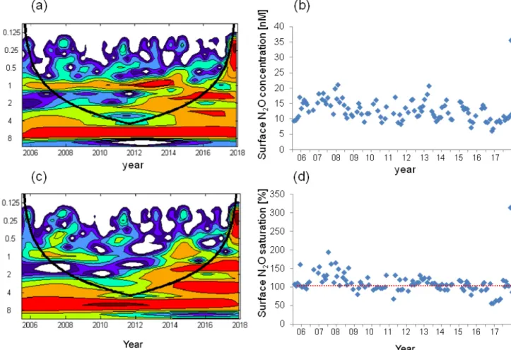
We found a weak seasonal cycle for surface N2O concentrations, with high N2O concentrations occurring in winter and early spring and low concentrations occurring in summer/autumn, but no such cycle for N₂O saturation (Figs. 4, 7). The seasonality in concentration but not in saturation could be largely attributed to the effect of temperature on N₂O solubility: in summer when surface N₂O concentrations are low, N₂O saturations are increased by the relative high temperature and vice versa in winter. Although salinity also affects N₂O solubility, its contribution is negligible compared to temperature. Temperature alleviated the fluctua-

(11)

Figure 7.Wavelet analysis and the variation in surface N₂O concentrations(a, b)and surface N₂O saturations(c, d). The dashed red line in (d)indicates the saturation of 100 %.

Figure 8. Variation of N₂O flux density at the BE Time Series- Station during 2005–2017. Negative values indicated N₂O influx from the atmosphere and positive values indicated N₂O efflux to the atmosphere.

tion of surface N₂O saturation and thus affected the sea-to-air N₂O fluxes. We conclude that temperature plays a modulating role for N₂O emissions.

The wind speed (u₁₀) at the BE Time Series Station ranged from 1.1 to 14.0 m s⁻¹, with an average of 7.0±2.7 m s⁻¹. N₂O flux densities varied from−19.0 to 105.7 µmol m⁻²d⁻¹

(−14.1 to 30.3 µmol m⁻²d⁻¹ without the extreme values), with an average of 3.5±12.4 µmol m⁻²d⁻¹ (3.3± 6.5 µmol m⁻²d⁻¹ without the extreme values). However, the true emissions might have been underestimated because our monthly sampling resolution is insufficient to capture short-term N2O accumulation events due to the fast breakdown of stratification in autumn. The uncertainty introduced in the flux density computation was estimated to be 20 % (Wanninkhof, 2014). The flux densities at the BE Time Se- ries Station are comparable to those reported by Bange et al. (1998, 0.4 to 7.1 µmol m⁻²d⁻¹) from the coastal waters of the southern Baltic Sea but are slightly lower than the average N₂O flux density reported by Rönner (1983, 8.9 µmol m⁻²d⁻¹) from the central Baltic Sea. Please note that the results of Rönner (1983) were obtained only from the summer season and therefore are probably biased because of missing seasonality.

In December 2014, a strong saline water inflow from the North Sea was observed, which was the third strongest ever recorded (Mohrholz et al., 2015). Although the salinity in December 2014 was comparable to other years, a remarkable increase in salinity was observed in the following several months. However, we did not detect a significant N2O

(12)

anomaly or enhanced emission during that time. Similarly, Walter et al. (2006) investigated the impact of the North Sea water inflow on N₂O production in the southern and central Baltic Sea in 2003. The oxygenated water ventilated the deep Baltic Sea and shifted anoxic to oxic condition which led to enhanced N₂O production, but the accumulated N₂O was un- likely to reach the surface due to the presence of a permanent halocline (Walter et al., 2006).

Although we observed an extremely high N₂O flux density in November 2017, the low-N₂O-concentration (< 10 nM) events have become more and more frequent during the past 12.5 years (Fig. 2). This phenomenon seldom occurred before 2011, but remarkable low N2O concentrations can be seen in 2011 and 2013, and to a lesser extent in 2012 and 2014. Similar events lasted for several months in 2015 and for even more than half a year during 2016–2017. The most striking feature was that the low-N₂O-concentration water was not only detected in bottom waters but also at surface which would significantly impact the air–sea N₂O flux densities. Although the MKT result did not give a significant trend for the N₂O flux densities, the data presented in Fig. 8 suggest a potential decline of N₂O flux densities from the coastal Baltic Sea, challenging the conventional view that N₂O emissions from coastal waters would most probably increase in the future, which was based on the hypothesis of increasing nutrient loads into coastal waters. Due to an effective reduction of nutrient inputs, the severe eutrophication condition in the Baltic Sea has been alleviated (HELCOM, 2018b), but ongoing deoxygenation points to the fact that it will take a longer time for coastal ecosystems to feedback to reduced nutrient inputs because other environmental changes such as warming may override decreasing eutrophication (Lennartz et al., 2014).

4 Conclusions

The seasonal and inter-annual N₂O variations at the BE Time Series Station from July 2005 to December 2017 were driven by the prevailing O₂ regime and nutrient availability. We found a pronounced seasonal cycle with low N₂O concentrations (undersaturations) occurring in hypoxic or anoxic bottom waters in autumn and enhanced concentrations (su- persaturations) all over the water column in winter and early spring. Significant decreasing trends for N2O concentrations were found for few months, while most of the year no significant trend was detectable in the period of 2005–2017. Dur- ing 2005–2017, no significant trends were present for O₂or nutrients either, but these parameters all show significant decreasing trends on longer timescales (∼60 years) at BE. Our results show the strong coupling of N₂O with O₂ and nutrient concentrations, and suggest similar changes on comparable timescales. Further monitoring of N₂O at BE Time Series Station is thus important to detect changes. Further studies on N₂O production and consumption by nitrification

and denitrification and analysis of the characteristic N2O iso- tope signature might be very helpful to decipher the potential roles of O₂and nutrients for N₂O cycling.

Temperature plays a modulating role for the N₂O emission at the BE Time Series Station. Although the hydrographic condition at BE is generally dominated by the inflow of saline North Sea water, this did not affect N₂O production and its emissions to the atmosphere. It seems that events with extremely low N₂O concentrations and thus reduced N₂O emissions became more frequent in recent years. Our results provide a new perspective on potential future patterns of N2O distribution and emissions in coastal areas. Continu- ous measurement at the BE Time Series Station with a focus on late autumn would be of great importance for monitoring and understanding the future changes in N2O concentrations and emissions in the southwestern Baltic Sea.

Data availability. Data are available from the Boknis Eck Database: https://www.bokniseck.de (Bange and Malien, 2019) and MEMENTO (the MarinE MethanE and NiTrous Oxide database, https://memento.geomar.de, Kock and Bange, 2015, last accessed:

23 October 2019).

Supplement. The supplement related to this article is available on- line at: https://doi.org/10.5194/bg-16-4097-2019-supplement.

Author contributions. XM, STL, and HWB designed the study and participated in the fieldwork. N₂O measurements and data process- ing were done by XM and STL. XM wrote the article with contributions from STL and HWB.

Competing interests. The authors declare that they have no conflict of interest.

Acknowledgements. The authors thank the captain and crew of the RVLittorinaandPolarfuchsas well as the many colleagues and nu- merous students who helped with the sampling and measurements of the BE time series through various projects. Special thanks to Anette Kock for her help with sampling, measurements, and data analysis. The time series at BE was supported by DWK Meeres- forschung (1957–1975), HELCOM (1979–1995), BMBF (1995–

1999), the Institut für Meereskunde (1999–2003), IfM-GEOMAR (2004–2011), and GEOMAR (2012–present). The current N₂O measurements at BE are supported by the EU BONUS INTEGRAL project which receives funding from BONUS (Art 185), funded jointly by the EU, the German Federal Ministry of Education and Research, the Swedish Research Council Formas, the Academy of Finland, the Polish National Centre for Research and Development, and the Estonian Research Council. The Boknis Eck Time Series Station (https://www.bokniseck.de, last access: 23 October 2019) is run by the Chemical Oceanography Research Unit of GEOMAR, Helmholtz Centre for Ocean Research Kiel.

(13)

X. Ma et al.: A multi-year observation of nitrous oxide 4109 Financial support. Xiao Ma is grateful to the financial support pro-

vided by the China Scholarship Council (grant no. 201306330056) and the BONUS INTEGRAL (grant no. 03F0773B).

Review statement. This paper was edited by S. Wajih A. Naqvi and reviewed by two anonymous referees.

References

Bange, H. W.: Nitrous oxide and methane in European coastal waters, Estuar. Coast. Shelf S., 70, 361–374, https://doi.org/10.1016/j.ecss.2006.05.042, 2006.

Bange, H. W., Dahlke, S., Ramesh, R., Meyer-Reil, L. A., Rapsomanikis, S., and Andreae, M. O.: Seasonal study of methane and nitrous oxide in the coastal waters of the southern Baltic Sea, Estuar. Coast. Shelf S., 47, 807–817, https://doi.org/10.1006/ecss.1998.0397, 1998.

Bange, H. W. and Malien, F.: Boknis Eck Timeseries Database, Kiel Datamanagement Team, http://www.bokniseck.de/, last accessed: 23 October 2019.

Battaglia, G. and Joos, F.: Marine N₂O emissions from nitrification and denitrification constrained by modern observations and projected in multimillenial global warming simulations, Global Biogeochem. Cy., 32, 92–121, https://doi.org/10.1002/2017GB005671, 2018.

Bonin, P., Gilewicz, M., and Bertrand, J. C.: Effects of oxygen on each step of denitrification on Pseudomonas nautica, Can. J. Mi- crobiol., 35, 1061–1064, https://doi.org/10.1139/m89-177, 1989.

Breitburg, D., Levin, L. A., Oschlies, A., Grégoire, M., Chavez, F.

P., Conley, D. J., Garçon, V., Gilbert, D., Gutiérrez, D., Isensee, K., Jacinto, G. S., Limburg, K. E., Montes, I., Naqvi, S. W. A., Pitcher, G. C., Rabalais, N. N., Roman, M. R., Rose, K. A., Seibel, B. A., Telszewski, M., Yasuhara, M., and Zhang, J.: De- clining oxygen in the global ocean and coastal waters, Science, 359, eaam7240, https://doi.org/10.1126/science.aam7240, 2018.

Capelle, D. W., Hawley, A. K., Hallam, S. J., and Tortell, P. D.: A multi-year time-series of N₂O dynamics in a seasonally anoxic fjord: Saanich Inlet, British Columbia, Limnol. Oceanogr., 63, 524–539, https://doi.org/10.1002/lno.10645, 2018.

Carstensen, J., Andersen, J. H., Gustafsson, B. G., and Con- ley, D. J.: Deoxygenation of the Baltic Sea during the last century, P. Natl. Acad. Sci. USA, 111, 5628–5633, https://doi.org/10.1073/pnas.1323156111, 2014.

Codispoti, L. A., Elkins, J. W., Yoshinari, T., Fredrich, G., Sakamoto, C., and Packard, T.: On the nitrous oxide flux from productive regions that contain low oxygen waters, in: Oceanog- raphy of the Indian Ocean, edited by: Desai, B. N., Oxford Univ.

Press, New York, 271–284, 1992.

Codispoti, L. A., Brandes, J. A., Christensen, J. P., Devol, A.

H., Naqvi, S. W. A., Paerl, H. W., and Yoshinari, T.: The oceanic fixed nitrogen and nitrous oxide budgets: Moving tar- gets as we enter the anthropocene?, Sci. Mar., 65, 85–105, https://doi.org/10.3989/scimar.2001.65s285, 2001.

Codispoti, L. A., Yoshinari, T., and Devol, A. H.: Suboxic respiration in the oceanic water column, in: Respiration in aquatic ecosystems, edited by: del Giorgio, P. A. and Williams, P. J., Ox- ford Univ. Press, New York, 225–247, 2005.

Conley, D. J., Carstensen, J., Aigars, J., Axe, P., Bonsdorff, E., Eremina, T., and Lannegren, C.: Hypoxia is increasing in the coastal zone of the Baltic Sea, Environ. Sci. Technol., 45, 6777–

6783, https://doi.org/10.1021/es201212r, 2011.

Cornejo, M., Murillo, A. A., and Farías, L.: An unaccounted for N₂O sink in the surface water of the eastern subtropical South Pacific: Physical versus biological mechanisms, Prog. Oceanogr., 137, 12–23, https://doi.org/10.1016/j.pocean.2014.12.016, 2015.

Dale, A. W., Sommer, S., Bohlen, L., Treude, T., Bertics, V. J., Bange, H. W., Pfannkuche, O., Schorp, T., Mattsdotter, M., and Wallmann, K.: Rates and regulation of nitrogen cycling in seasonally hypoxic sediments during winter (Boknis Eck, SW Baltic Sea): Sensitivity to environmental variables, Estuar. Coast. Shelf S., 95, 14–28, https://doi.org/10.1016/j.ecss.2011.05.016, 2011.

Ducklow, H. W., Doney, S. C., and Steinberg, D. K.: Contributions of long-term research and time-series observations to marine ecology and biogeochemistry, Annu. Rev. Mar. Sci., 1, 279–302, https://doi.org/10.1146/annurev.marine.010908.163801, 2009.

Farías, L., Castro-González, M., Cornejo, M., Charpentier, J., Faún- dez, J., Boontanon, N., and Yoshida, N.: Denitrification and nitrous oxide cycling within the upper oxycline of the eastern tropi- cal South Pacific oxygen minimum zone, Limnol. Oceanogr., 54, 132–144, https://doi.org/10.4319/lo.2009.54.1.0132, 2009.

Farías, L., Faúndez, J., Fernández, C., Cornejo, M., Sanhueza, S., and Carrasco, C.: Biological N₂O fixation in the Eastern South Pacific Ocean and marine cyanobacterial cultures, Plos One, 8, e63956, https://doi.org/10.1371/journal.pone.0063956, 2013.

Farías, L., Besoain, V., and García-Loyola, S.: Presence of nitrous oxide hotspots in the coastal upwelling area off central Chile: an analysis of temporal variability based on ten years of a biogeochemical time series, Environ. Res. Lett., 10, 044017, https://doi.org/10.1088/1748-9326/10/4/044017, 2015.

Goreau, T. J., Kaplan, W. A., Wofsy, S. C., McElroy, M. B., Valois, F. W., and Watson, S. W.: Production of NO⁻₂ and N₂O by nitri- fying bacteria at reduced concentrations of oxygen, Appl. Envi- ron. Microb., 40, 526–532, 1980.

Grasshoff, K., Kremling, K., and Ehrhardt, M.: Methods of seawater analysis, 3rd edition, WILEY-VCH, Weihheim, Germany, 208–

225, 1999.

Hannig, M., Lavik, G., Kuypers, M. M. M., Woebken, D., Martens- Habbena, W., and Jürgens, K.: Shift from denitrification to anammox after inflow events in the central Baltic Sea, Limnol.

Oceanogr., 52, 1336–1345, 2007.

Hansen, H. P., Giesenhagen, H. C., and Behrends, G.: Seasonal and long-term control of bottom water oxygen deficiency in a stratified shallow-coastal system, ICES J. Mar. Sci., 56, 65–71, https://doi.org/10.1006/jmsc.1999.0629, 1999.

HELCOM: Sources and pathways of nutrients to the Baltic Sea, Baltic Sea Environ. Proc., 153, 4–46, 2018a.

HELCOM: State of the Baltic Sea – Second HELCOM holistic assessment 2011–2016, Baltic Sea Environ. Proc., 155, 41–58, 2018b.

Hietanen, S. and Lukkari, K.: Effects of short-term anoxia on benthic denitrification, nutrient fluxes and phosphorus forms in coastal Baltic sediment, Aquat. Microb. Ecol., 49, 293–302, https://doi.org/10.3354/ame01146, 2007.

Hsu, S. A., Meindl, E. A., and Gilhousen, D. B.: Determining the power-law wind-profile exponent under near-neutral stabil- ity conditions at sea, J. Appl. Meteorol., 33, 757–765, 1994.

(14)

IPCC: Climate Change 2013: The physical science basis. Contri- bution of Working Group I to the fifth assessment report of the Intergovernmental Panel on Climate Change, Cambridge Univer- sity Press, Cambridge, UK and New York, NY, 467–552, 2013.

Kock, A. and Bange, H. W.: Counting the ocean’s greenhouse gas emissions, Eos (Washington DC), 96, 10–13, https://doi.org/10.1029/2015EO023665, 2015.

Kock, A., Arévalo-Martínez, D. L., Löscher, C. R., and Bange, H. W.: Extreme N₂O accumulation in the coastal oxygen minimum zone off Peru, Biogeosciences, 13, 827–840, https://doi.org/10.5194/bg-13-827-2016, 2016.

Kroeze, C. and Seitzinger, S. P.: Nitrogen inputs to rivers, estuar- ies and continental shelves and related nitrous oxide emissions in 1990 and 2050: a global model, Nutr. Cycl. Agroecosys., 52, 195–212, 1998.

Kulkarni, A. and Von Storch, H.: Monte Carlo experiments on the effect of serial correlation on the Mann-Kendall test of trend, Me- teorol. Z., 4, 82–85, 1995.

Landolfi, A., Somes, C. J., Koeve, W., Zamora, L. M., and Os- chlies, A.: Oceanic nitrogen cycling and N₂O flux perturbations in the Anthropocene, Global Biogeochem. Cy., 31, 1236–1255, https://doi.org/10.1002/2017GB005633, 2017.

Lennartz, S. T., Lehmann, A., Herrford, J., Malien, F., Hansen, H. P., Biester, H., and Bange, H. W.: Long-term trends at the Boknis Eck time series station (Baltic Sea), 1957–2013:

does climate change counteract the decline in eutrophication?, Biogeosciences, 11, 6323–6339, https://doi.org/10.5194/bg-11- 6323-2014, 2014.

Löscher, C. R., Kock, A., Könneke, M., LaRoche, J., Bange, H.

W., and Schmitz, R. A.: Production of oceanic nitrous oxide by ammonia-oxidizing archaea, Biogeosciences. 9, 2419–2429, https://doi.org/10.5194/bg-9-2419-2012, 2012.

Martinez-Rey, J., Bopp, L., Gehlen, M., Tagliabue, A., and Gruber, N.: Projections of oceanic N₂O emissions in the 21st century using the IPSL Earth system model, Biogeosciences, 12, 4133–

4148, https://doi.org/10.5194/bg-12-4133-2015, 2015.

Meier, H. M., Väli, G., Naumann, M., Eilola, K., and Frauen, C.:

Recently accelerated oxygen consumption rates amplify deoxygenation in the Baltic Sea, J. Geophys. Res.-Ocean., 123, 3227–

3240, https://doi.org/10.1029/2017JC013686, 2018.

Mohrholz, V., Naumann, M., Nausch, G., Krüger, S., and Gräwe, U.: Fresh oxygen for the Baltic Sea-An exceptional saline inflow after a decade of stagnation, J. Marine Syst., 148, 152–166, https://doi.org/10.1016/j.jmarsys.2015.03.005, 2015.

Naqvi, S. W. A., Jayakumar, D. A., Narvekar, P. V., Naik, H., Sarma, V. V. S. S., D’souza, W., Joseph, S., and George, M. D.: Increased marine production of N₂O due to intensifying anoxia on the In- dian continental shelf, Nature, 408, 346–349, 2000.

Naqvi, S. W. A., Bange, H.W., Farías, L., Monteiro, P. M. S., Scranton, M. I., and Zhang, J.: Marine hypoxia/anoxia as a source of CH₄ and N₂O, Biogeosciences, 7, 2159–2190, https://doi.org/10.5194/bg-7-2159-2010, 2010.

Nevison, C., Butler, J. H., and Elkins, J. W.: Global distribution of N₂O and the 1N₂O-AOU yield in the subsurface ocean, Global Biogeochem. Cy., 17, 1119, https://doi.org/10.1029/2003GB002068, 2003.

Nightingale, P., G. Malin, C. S. Law, A. J. Watson, P. S. Liss, M. I.

Liddicoat, J. Boutin, and R. C. Upstill-Goddard: In situ evalua- tion of air-sea gas exchange parameterizations using novel con-

servative and volatile tracers, Global Biogeochem. Cy., 14, 373–

387, https://doi.org/10.1029/1999GB900091, 2000.

Rabalais, N. N., Cai, W.-J., Carstensen, J., Conley, D. J., Fry, B., Hu, X., Quinones-Rivera, Z., Rosenberg, R., Slomp, C. P., Turner, R.

E., Voss, M., Wissel, B., and Zhang, J.: Eutrophication-driven deoxygenation in the coastal ocean, Oceanography, 27, 172–183, https://doi.org/10.5670/oceanog.2014.21, 2014.

Ravishankara, A. R., Danielm J., S., and Portmann, R. W.:

Nitrous oxide (N₂O): the dominant ozone-depleting sub- stance emitted in the 21st century, Science, 326, 123–125, https://doi.org/10.1126/science.1176985, 2009.

Rönner, U.: Distribution, production and consumption of nitrous oxide in the Baltic Sea, Geochim. Cosmochim. Ac., 47, 2179–

2188, https://doi.org/10.1016/0016-7037(83)90041-8, 1983.

Schlittgen, R. and Streitberg, B. H. J.: Zeitreihenanalyse, Oldenburg Wissenschaftsverlag, Munich, Germany, 1–89, 2001.

Seitzinger, S. P. and Kroeze, C.: Global distribution of nitrous oxide production and N inputs in freshwater and coastal marine ecosystems, Global Biogeochem. Cy., 12, 93–113, 1998.

Siedler, G. and Peters, H.: Properties of sea water, in: Oceanogra- phy, edited by Sündermann J., Springer, Berlin, Heidelberg, 233–

264, 1986.

Simone, F.: Mann-Kendall Test, MathWorks, https:

//ww2.mathworks.cn/matlabcentral/fileexchange/

25531-mann-kendall-test (last access: 23 October 2019), 2009.

Sohm, J. A., Webb, E. A., and Capone, D. G.: Emerging patterns of marine nitrogen fixation, Nat. Rev. Microbiol., 9, 499–508, https://doi.org/10.1038/nrmicro2594, 2011.

Tiedje, J. M.: Ecology of denitrification and dissimilatory nitrate reduction to ammonium, in: Environmental Microbiology of Anaerobes, edited by: Zehnder, A. J. B., John Wiley & Sons, NY, 179–244, 1988.

Torrence, C. and Compo, G. P.: A practical guide to wavelet analysis, B. Am. Meteorol. Soc., 79, 61–78, 1998.

Torrence, C. and Compo, G. P.: Wavelet analysis, http://paos.

colorado.edu/research/wavelets/ (last access: 23 October 2019), 2004.

Voss, M., Emeis, K. C., Hille, S., Neumann, T., and Dipp- ner, J. W.: Nitrogen cycle of the Baltic Sea from an iso- topic perspective, Global Biogeochem. Cy., 19, GB3001, https://doi.org/10.1029/2004GB002338, 2005.

Walter, S., Breitenbach, U., Bange, H. W., Nausch, G., and Wal- lace, D. W.: Distribution of N₂O in the Baltic Sea during transi- tion from anoxic to oxic conditions, Biogeosciences, 3, 557–570, https://doi.org/10.5194/bg-3-557-2006, 2006.

Wanninkhof, R.: Relationship between wind speed and gas exchange over the ocean revisited, Limnol. Oceanogr.-Method., 12, 351–362, https://doi.org/10.4319/lom.2014.12.351, 2014.

Weiss, R. F. and Price, B. A.: Nitrous oxide solubility in water and seawater, Mar. Chem., 8, 347–359, https://doi.org/10.1016/0304- 4203(80)90024-9, 1980.

Wilson, S. T., Ferrón, S., and Karl, D. M.: Interannual variability of methane and nitrous oxide in the North Pa- cific Subtropical Gyre, Geophys. Res. Lett., 44, 9885–9892, https://doi.org/10.1002/2017GL074458, 2017.

Xu, Z. X., Takeuchi, K., and Ishidaira, H.: Monotonic trend and step changes in Japanese precipitation, J. Hydrol., 279, 144–150, https://doi.org/10.1016/S0022-1694(03)00178-1, 2003.

(15)

X. Ma et al.: A multi-year observation of nitrous oxide 4111 Yang, D., Li, C., Hu, H., Lei, Z., Yang, S., Kusuda, T., Koike,

T., and Musiake, K.: Analysis of water resources variability in the Yellow river of China during the last half century using the historical data, Water Resour. Res., 40, 1–12, https://doi.org/10.1029/2003WR002763, 2004.

Zhang, G.-L., Zhang, J., Liu, S.-M., Ren, J.-L., and Zhao, Y.- C.: Nitrous oxide in the Changjiang (Yangtze River) estu- ary and its adjacent marine area: Riverine input, sediment re- lease and atmospheric fluxes, Biogeosciences, 7, 3505–3516, https://doi.org/10.5194/bg-7-3505-2010, 2010.