Praktikum Quantenphysik 141.A12 Pulsed Nuclear Magnetic Resonance

Helmut Hörner, Samuel Rind, Sita Schönbauer

Praktikum Quantenphysik 141.A12 Pulsed Nuclear Magnetic Resonance

Lab Report

(Rev. 2)

Vienna University of Technology Institute of Atomic and Subatomic Physics

Vienna, May 2019

Contents

1 Introduction 3

2 Experiments 3

2.1 Lamor Frequency of Protons in the Hydrogen Atoms of Mineral Oil . . . 3

2.1.1 Theory and Experimental Setup . . . . 3

2.1.2 Experimental Results . . . . 4

2.2 Fine-Tuning the Magnetic Field . . . . 5

2.2.1 Theory and Experimental Setup . . . . 5

2.2.2 Experimental Results . . . . 5

2.3 Manipulating Spin Orientation by Applying Pulses of According Length . 5 2.3.1 Theory and Experimental Setup . . . . 5

2.3.2 Experimental Results . . . . 6

2.4 Inhomogeneous Traverse Relaxation Time T

. . . . 7

2.4.1 Theory and Experimental Setup . . . . 7

2.4.2 Experimental Results . . . . 7

2.5 Spin-Lattice Relaxation Time T

. . . . 8

2.5.1 Theory and Experimental Setup . . . . 8

2.5.2 Experimental Results . . . . 9

2.6 Homogeneous Traverse Relaxation Time T

. . . 10

2.6.1 Theory and Experimental Setup . . . 10

2.6.2 Experimental Results . . . 11

2.7 Measuring T

with Multiple Pulse Sequences . . . 13

2.7.1 Theory and Experimental Setup . . . 13

2.7.2 Experimental Results . . . 13

3 Appendix 15

1 Introduction

The experiments described in this report were carried out by Samuel Rind, Sita Schön- bauer and Helmut Hörner on May 9, 2019 at the Institute of Atomic and Subatomic Physics of the Vienna University of Technology as part of the course "Praktikum Quan- tenphysik 141.A12". The experiments demonstrate the principles of nuclear magnetic resonance (NMR).

2 Experiments

2.1 Lamor Frequency of Protons in the Hydrogen Atoms of Mineral Oil 2.1.1 Theory and Experimental Setup

In this series of experiments, mineral oil was exposed to a static, homogeneous magnetic field B ~

= B

~ e

of a NdFeB permanent magnet. As the liquid consists of hydrocarbons, in which the

C nuclei have no spin, this leads to a precession of the spins of the protons in the hydrogen atoms around the z-axis with the angular Lamor frequency

ω

= γB

(1)

When exposed to such a magnetic field, spins aligned along the applied magnetic field B ~

have a lower energy than spins pointing in the opposite direction, with the energy difference being ∆ E =

ω ("Nuclear Zeeman Effect"). The difference in population be- tween these two states is only on the ppm order, but yet strong enough to be observed as a net magnetization M ~

.

In this experimental setup, in addition to the static B ~

field, also a pair of Helmholtz- coils (integrated in [PS2 RF Sample Probe]) was placed around the sample so that it could be exposed to RF pulses B ~

= B

cos ( ωt ) ~ e

perpendicular to the B ~

field (hereby defining the as x-axis).

When ω = ω

, then there is resonance, and the effect of the (comparably small) B ~

field can accumulate with every full precession cycle and can hence give rise to a large change in the spin state, and consequently in the net magnetization vector (see [Levitt 2008, p.247]). For example, if the RF pulse is timed so that t

ω

=

, then the net magneti- zation vector will be processing around the equator at the Lamor frequency ("

-pulse").

Similarly, a π -pulse will move the net magnetization vector further towards the negative z-direction, and so on.

The precessing spins induce an electric current in the Helmholtz-coils (which also dub as

detectors). This signal is maximal when the rotation axis of the net magnetic momen-

tum lies perpendicular to the magnetic axis of the coils, i.e. when the net magnetization

vector is processing around the equator.

The Helmholtz Coils in [PS2 RF Sample Probe] were connected to a [PS2 Mainframe]

programmable pulse sequence RF pulse generator.

The current induced by the protons RF-field was processed into two separate signals, which where displayed in parallel by a [DSO-X 2012A] oscilloscope: On channel 1, the

was displayed, and on channel 2 the

between the RF-pulse emitted into the sample and the RF-pulse received from the sample was displayed.

The pulse generator [PS2 Mainframe] was set to generate 1 µs pulses with a 300 ms period (to allow complete thermalization between the pulses). The oscilloscope trigger input was connected to the pulse generator.

2.1.2 Experimental Results

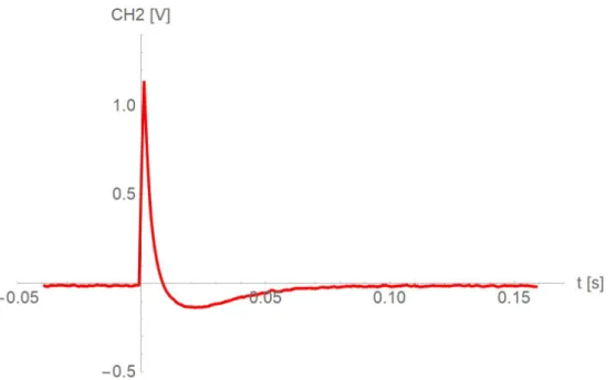
On channel 2 of the [DSO-X 2012A] oscilloscope (showing the phase difference between emitted and received signal), a damped oscillation, representing the beat between the precessing magnetization vector and the RD frequency applied in the pulse, became visible. The frequency of the RF pulse generator was tuned until the beat oscillation vanished.

Figure 1: Beat oscillation vanished after RF pulses tuned to Lamor frequency

The resonance frequency was measured to be

f

= f

= 21 . 524 19 MHz (2)

Considering that ω

= 2 πf

, equation (1) can be rearranged to B

= 2 πf

γ (3)

With the gyromagnetic ratio of the proton being γ = 267.522

10

, the value of the magnetic field B ~

can be calculated to be

B

= 0 . 506 T (4)

2.2 Fine-Tuning the Magnetic Field 2.2.1 Theory and Experimental Setup

To make the magnetic field B ~

as homogeneous over the volume of the sample as possible, gradient coils were placed alongside the permanent magnet. These gradient coils were connected to the [PS2 Controller], which allows for tuning the linear magnetic field gradients along all three axes, as well as for the quadratic filed component along the z-axis. The field is most homogeneous when the envelope signal on channel 1 has the maximum length.

2.2.2 Experimental Results

It turned out that the setting of the [PS2 Controller] was already almost optimal. There- fore, there is only a minuscule difference in the determined value for the Lamor frequency after this tuning step.

f

= f

= 21 . 524 47 MHz (5)

2.3 Manipulating Spin Orientation by Applying Pulses of According Length 2.3.1 Theory and Experimental Setup

In this experiment, we varied the pulse length between 0 µs and 20 µs with a 300 ms period (to allow complete thermalization between the pulses). For each pulse length the immediate peak amplitude of the signals in channel 1 and channel 2 was recorded.

With increasing pulse length, the net magnetization vector moves towards the equator and hence the envelope signal in channel 1 increases from zero to maximum until the

π

2

pulse length is reached. Then the signal strength is expected to decrease to a mini-

mum until the pulse length reaches π pulse length. This cycle then continues with

and

2 π pulse length. Hence, tuning the pulse length from 0 to 2 π results in two signal periods.

In contrast, the phase signal in channel 2 is expected to show only one full period when tuning the pulse length from 0 to 2 π pulses.

2.3.2 Experimental Results

Table 1 shows the measured values. As can be seen, two extra measurements were per- formed "outside" the constant grid to determine the exact pulse lengths for the channel 2 phase signal to become zero. This allows for the most precise calculation of the

signal length.

Pulse Length CH 1 Envelope CH2 Phase Diff.

µs V V

0.0 0.000 0.000

1.0 4.188 0.631

2.0 7.250 1.100

4.0 9.870 1.488

6.0 7.750 1.110

8.0 1.000 0.112

8.2 - 0.000

10.0 5.562 -1.000

12.0 8.560 -1.480

14.0 7.630 -1.260

16.0 2.200 -0.410

16.8 - 0.000

18.0 4.080 0.580

20.0 7.250 1.060

Table 1: Signal strength and signal phase difference vs. pulse length

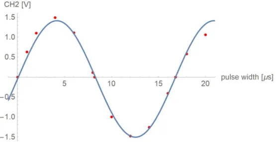
Figure 2: Phase sensitive signal for various pulse widths

As a pulse width of 16 . 8 µs concludes a full period in the channel 2 phase signal (equaling to a 2 π pulse, see table 1), the

pulse length can easily be calculated to be

t

= t

4 = 16 . 8

4 = 4 . 2 µs (6)

2.4 Inhomogeneous Traverse Relaxation Time T

2.4.1 Theory and Experimental Setup

As the microscopic environment of each nucleus is slightly different, each nucleus has consequently a slightly different Lamor frequency. This means that, after a

pulse, the spin vectors will spread out more and more over time, until coherence is lost. Further- more, the applied magnetic field B ~

is not entirely homogeneous which in total leads to an even increased decoherence speed, characterized by the traverse relaxation time T

M

= M

e

(7)

The traverse relaxation time T

can be determined by exposing the sample to

pulses, and fitting equation 5 to the measured envelope signal on channel 1.

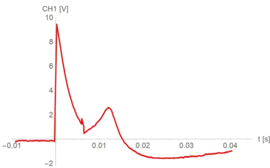
2.4.2 Experimental Results

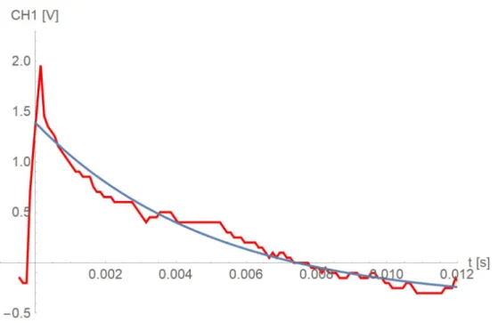
Figure 3: Exponential decay after a

pulse (red) and fit function

0.4 + 1.79e

As figure 3 shows, the measured decay in the envelope signal on channel 1 had a certain bias, so that the signal dropped below zero when leveling out. This was accounted for by extending fit-function (7) with a fixed offset of

0 . 4.

The best-fit function, for which the parameters were determined employing the Nonlin- earModelFit method of Mathematica 11.3., is

0 . 4 + 1 . 79 e

. From this fit function, the estimated traverse relaxation time can be determined to be

T

= 5 ms (8)

2.5 Spin-Lattice Relaxation Time T

2.5.1 Theory and Experimental Setup

The previous measurement did not reflect the actual spin-lattice relaxation time T

, as it was affected by unavoidable inhomogeneities in the magnetic field B ~

. This problem can be circumvented by the "inverse recovery T

pulse sequence", employed in the next measurement: In the first step, the sample is exposed to a π pulse, which turns all spins into negative z direction. As time passes, the spins will begin to rotate back towards positive z-direction, ever more spreading out around all ϕ angles.

Then, after as specific time τ , a further

pulse is emitted into the sample. This brings the rotating net spin vector to the traverse plane. The projection of the net spin into the xy-plane however will depend on the amount of decoherence the individual spin vectors have experienced in the time τ between the π pulse and the

pulse. First, the projection of the net spin into the xy-plane will get ever smaller with growing τ . When the

pulse hits exactly at the moment when the spins have decoherently spread out and moved to the traverse plane anyway ("zero crossing time"), the projection of the net spin into the xy-plane after the

will be exactly zero.

This means that the phase sensitive signal on channel 2 is expected to start with large negative values for short values of τ and will become ever closer to zero until τ reaches the zero-crossing time. After that, the phase sensitive signal on channel 2 will become positive.

The intensity of the signal is described by

M ( t ) = M

(1

2 e

) (9) The intensity is zero at τ

= T

log (2), so that T

can easily be determined by mea- suring the zero-crossing time τ

T

= τ

log (2) (10)

2.5.2 Experimental Results

Table 2 shows the results of the inverse recovery T

pulse sequence measurement.

τ CH2 peak

ms V

0,1 -1,46 5,0 -1,09 10,0 -0,66 15,0 -0,34 20,0 -0,16 25,0 0,00 30,0 0,19 35,0 0,39 40,0 0,51 45,0 0,63

Table 2: Inverse recovery T

pulse sequence measurement

As can be seen in this table, the zero-crossing time τ

= 25 ms. Employing relation (10), the spin-lattice replaxation time can be calulated to be

T

= 25 ms

log (2) = 36 ms (11)

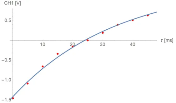
The following figure 4 visualizes the complete data set and the matching fit-function

−

0 . 4+1 . 79 e

(parameter determined with the NonlinearModelFit method of Math- ematica 11.3).

Figure 4: Inverse recovery T

pulse sequence measurement; fit-function 1 . 43(1

2 e

)

According to the fit-function displayed in above graph, the spin-lattice relaxation time can be estimated to be

T

= 34 . 7 ms (12)

2.6 Homogeneous Traverse Relaxation Time T

2.6.1 Theory and Experimental Setup

To determine the exact traverse relaxation time T

without having inhomogenities in the magnetic field B ~

affecting the measurement (as in the measurement of T

), the following method was applied:

With a first

pulse, the net magnetization was rotated into the equatorial plane. Next, after a certain time τ during the decay, the sample was exposed to another π pulse.

This leads to a re-phasing of the spins, visible in so-called "Hahn-Echos" in the envelope signal of channel 1 (see figure 5).

By varying the delay time τ , Hahn-echos of different peak amplitudes can be generated.

When the peak values of these Hahn-echos are plotted over τ , and this plot is then fitted by equation 13, the exponent parameter T

of the fitting function gives a good estimation of the actual homogeneous traverse relation time.

M

= M

e

(13)

2.6.2 Experimental Results

Figure 5 shows an exemplary Hahn echo after a delay time τ = 6 ms

Figure 5: Exemplary Hahn echo after τ = 6 ms in the envelope signal on channel 1

τ CH1 peak

ms V

2,0 5,60 4,0 4,02 6,0 2,80 6,2 2,77 8,0 2,10 10,0 1,57 12,0 1,20 14,0 0,97 16,0 0,80 18,0 0,67 20,0 0,57

Table 3: Magnitude of Hahn echos over different delay times τ

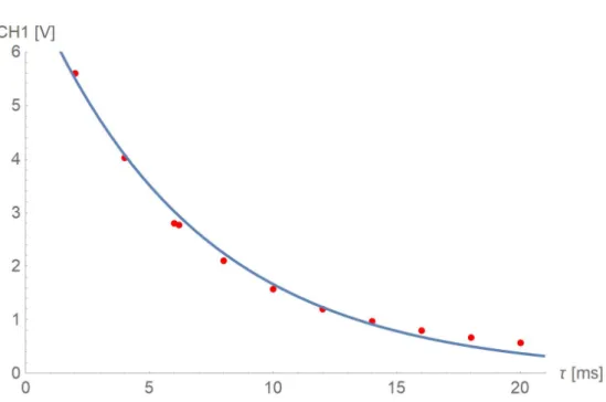
The following figure 6 visualizes the complete data set of table 3 and the matching

fit-function 7.4e

(parameter determined with the NonlinearModelFit method of

Mathematica 11.3).

Figure 6: Magnitude of Hahn echo vs. delay time τ ; fit-function 7 . 4 e

From this fit-function, the homogeneous traverse relaxation time T

can be determined to be

T

= 6.7 ms (14)

which is, as expected, longer than the previously measured inhomogeneous traverse re- laxation time T

= 5 ms.

The relationship between T

and "T

is given by 1

T

= 1

T

γ ∆ B

2 (15)

with ∆ B

being the magnetic field inhomogeneity. Equation (15) can be re-arranged to

∆ B

= 2 γ

1

T

1 T

(16) Hence, the magnetic field inhomogeneity in our experiment was

∆ B

= 2

267 . 522

10

1

0 . 005

1 0 . 0067

= 379 nT (17)

2.7 Measuring T

with Multiple Pulse Sequences 2.7.1 Theory and Experimental Setup

A refinement of the Hahn echo method was described by [Carr and Purcell, 1954]. In this scheme, a first

pulse is followed by a series of π pulses. If the time interval between the first

and second π pulse is τ , then the interval between all further impulses has to be 2 τ . Echos are observed midway between the π pulses, and the amplitude of successive echos decays exponentially with a time constant equal to T

.

However, with this method the exact adjustment of the π pulses is crucial, because even small deviations from the exact value gives rise to cumulative errors in the result. This is in conflict with the requirement that the number of π pulses should be large in order to eliminate the effects of diffusion.

An improved pulse sequence named "CPMG" after their developers Carr, Purcell, Mei- book and Gill, described in [Meiboom and Gill, 1958], solves this problem. The pulse sequence differs from the method described by [Carr and Purcell, 1954] in two respects:

(i) The successive pulses are coherent, and (ii) the phase of the

pulse is shifted by

pulse relative to the pase of the π pulses.

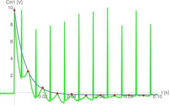
2.7.2 Experimental Results

We programmed the [PS2 Mainframe] to the CPMG sequence with τ = 5 ms. Fig- ure 7 visualizes the Hahn echos produced by this sequence and the matching fit-function

−

0 . 28 + 9 . 97 e

(parameter determined with the NonlinearModelFit method of Mathematica 11.3).

The time constant extracted from the fit-function gives the T

value to be

T

= 7 . 5 ms (18)

Figure 7: CPMG pulse sequence ( τ = 5 ms); fit-function

0 . 28 + 9 . 97 e

3 Appendix

Equipment

[PS2 Controller] Current regulated supply for gradient coils TeachSpin PS2 Controller [PS2 Mainframe] Pulse Programmer/Synthesizer/Receiver unit TeachSpin PS2 Mainframe [PS2 RF Sample Probe] Single coil RF sample probe TeachSpin PS2 RF probe

[DSO-X 2012A] Oscilloscope Keysight InfiniiVision DSO-X 2012A

List of Tables

1 Signal strength and signal phase difference vs. pulse length . . . . 6 2 Inverse recovery T

pulse sequence measurement . . . . 9 3 Magnitude of Hahn echos over different delay times τ . . . 11

List of Figures

1 Beat oscillation vanished after RF pulses tuned to Lamor frequency . . . 4 2 Phase sensitive signal for various pulse widths . . . . 6 3 Exponential decay after a

pulse (red) and fit function

0.4 + 1.79e

7 4 Inverse recovery T

pulse sequence measurement; fit-function 1 . 43(1

2 e

) . . . . 9 5 Exemplary Hahn echo after τ = 6 ms in the envelope signal on channel 1 . 11 6 Magnitude of Hahn echo vs. delay time τ ; fit-function 7 . 4 e

. . . 12 7 CPMG pulse sequence ( τ = 5 ms); fit-function

0 . 28 + 9 . 97 e

. . . 14

References

[Carr and Purcell, 1954] Carr, H. Y., Purcell, E. M.; Effects of Diffusion on Free Precession in Nuclear Magnetic Resonance Ex- periments. Physical Review. 94, 1954, p. 630–638.

DOI:10.1103/PhysRev.94.630

[Levitt 2008] Malcom J. Levitt: Spin Dynamics; Basics of Nuclear Mag- netic Resonance, 2nd edition, 2008. John Wiley, Chichester.

[Meiboom and Gill, 1958] S. Meiboom and D. Gill; Modified Spin-Echo Method for Measuring Nuclear Relaxation Times, Rev. Sci. Instrum.

29, 688 (1958), DOI: 10.1063/1.1716296