An Analytic Derivation of the Efficient Surface in Portfolio Selection with Three Criteria

An Analytic Derivation of the Efficient Surface in Portfolio Selection with Three Criteria

Yue Qi

Department of Financial Management, Business School Nankai University

Tianjin, 300071, China Ralph E. Steuer Department of Finance

University of Georgia Athens, GA, 30602-6253, U.S.A.

Maximilian Wimmer Department of Finance University of Regensburg 93040 Regensburg, Germany

Abstract

In standard mean-variance bi-criterion portfolio selection, the efficient

set is a frontier. While it is not yet standard for there to be additional cri-

teria in portfolio selection, there has been a growing amount of discussion

in the literature on the topic. However, should there be even one additional

criterion, the efficient frontier becomes an efficient surface. Striving to par-

allel Merton’s seminal analytical derivation of the efficient frontier, in this

paper we provide an analytical derivation of the efficient surface when an ad-

ditional linear criterion (on top of expected return and variance) is included

in the model addressed by Merton. Among the results of the paper there is,

as a higher dimensional counterpart to the 2-mutual-fund theorem of tradi-

tional portfolio selection, a 3-mutual-fund theorem in tri-criterion portfolio

selection. 3D graphs are employed to stress the paraboloidic/hyperboloidic

structures present in tri-criterion portfolio selection.

1 Introduction

In investments, portfolio selection is the problem of allocating a given sum of money to securities drawn from a designated pool of securities for the purpose of maximizing the future return of the portfolio thus formed, or, that is, for the purpose of maximizing portfolio return. With portfolio return a random variable, the foundation for the solution of the problem of portfolio selection was laid out by Markowitz (1952) in the form of his famous mean–variance model. In this model, “mean” refers to the endeavor to maximize the expected return of the port- folio return random variable, and “variance,” which is Markowitz’s measure for risk, refers to the endeavor to minimize the variance of the portfolio return random variable. Hence the so-called mean–variance model is a bi-criterion optimization problem with as its two objectives variance to be minimized and expected return to be maximized.

While mean–variance has maintained its status as the predominant model in portfolio selection for over sixty years, it has not been without attempts to extend its scope. One such attempt arose in the 1970s. It is the attempt to include in the portfolio selection process a criterion beyond expected return and variance. Lee (1972) proposed taking dividends into account along with expected return and vari- ance when constructing a portfolio. Stone (1973) proposed skewness as a different kind of third criterion possibility. With only occasional articles on this following, one such being by Spronk and Zambruno (1981), the idea of additional criteria in portfolio selection essentially remained on the back burner of portfolio selec- tion until the mid-1990s when, for instance, Konno and Suzuki (1995) revisited skewness, Chow (1995) considered tracking error as a third criterion, and Sper- anza (1996) and others mentioned in different ways transaction costs. Soon several survey-type articles appeared such as by Spronk and Hallerbach (1997), Bana e Costa and Soares (2001), and Steuer and Na (2003) giving further impetus to the idea of additional objectives.

While skewness and tracking error are difficult to implement because of their

nonlinearities, additional criteria that can be modeled linearly are much more trac-

table. Recognizing this, the literature then saw a string of contributions involving

linear criteria whose number has only been increasing. For example, Lo, Petrovz

and Wierzbicki (2003) examined liquidity in this regard, considered social respon-

sibility, and Ehrgott, Klamroth and Schwehm (2004) took into account the star

ranking of a mutual fund. In the list contained in Steuer, Qi and Hirschberger

(2007), the amount invested in R&D (see Guerard and Mark, 2004) and growth-

in-sales (Ziemba, 2006) are also enumerated as possible additional criteria. On

the methodological front of how to handle additional criteria in portfolio selection,

there are among others the offerings by Ben Abdelaziz, Aouni and Fayedh (2007),

Hirschberger, Steuer, Utz, Wimmer and Qi (2013), Aouni, Colapinto and La Torre (2014), and Xidonas, Mavrotas, Krintas and Psarras (2012).

However, as of most recently, the additional criterion that appears to be attract- ing the most attention is social responsibility. Another term often used interchange- ably with social responsibility is sustainability. Over the past few years many pa- pers have been written about social responsibility in portfolio selection includ- ing those by Ballestero, Bravo, P´erez-Gladish, Arenas-Parra and Pl`a-Santamaria (2012), Dorfleitner, Leidl and Reeder (2012), Bilbao-Terol, Arenas-Parra, Ca˜nal- Fern´andez and Bilbao-Terol (2013), Calvo, Ivorra and Liern (2014), Cabello, Ruiz, P´erez-Gladish and M´endez-Rodriguez (2013), P´erez-Gladish, M´endez-Rodriguez, M’Zali and Lang (2013), Utz, Wimmer, Hirschberger and Steuer (2014), and Utz, Wimmer and Steuer (2015).

While substantial progress has been made as described above, it is quite possi- ble that multiple criteria in portfolio selection is still in its early stages. With cri- teria beyond expected return and variance causing the efficient frontier to become an efficient surface, many new questions about the structure of the efficient surface and its relationship to other key quantities in portfolio selection arise. While it is certainly possible to compute individual efficient solutions by means of inserting any additional criterion into the problem as a constraint, this only generates partial information. But to appreciate the full expanse of potentially optimal choices of- fered by a problem, it is necessary to compute the entire efficient surface. Whereas Merton (1972) has provided a very nice analytical derivation of the bi-criterion efficient frontier of traditional portfolio selection, the purpose of this paper is to provide a similar analytical derivation but of the efficient surface of a tri-criterion portfolio selection problem.

The paper is organized as follows. In Section 2 we touch on multiple criteria

optimization and summarize many of the main results of the efficient frontier of

Merton’s model. In Section 3 we formulate our tri-criterion model and analytically

derive the minimum-variance surface. In Section 4 we derive the portion of the

minimum-variance surface that is the efficient surface, and in Section 5 we provide

an illustrative numerical example. Also in Section 5, we are able to illustrate the

paraboloidic/hyperboloidic nature of the efficient surface by means of several 3D

graphs.

2 Multiple criteria optimization and portfolio selection

We briefly review multiple criteria optimization and portfolio selection models in this section. A multiple objective optimization problem can be formulated as

max { z

= f

( x )} (1)

...

max { z

= f

(x)}

s.t. x ∈ S

where k is the number of objectives and S ⊂ R

is the feasible region in decision space. Because (1) has more than one objective, there is another version of the feasible region, that being Z ⊂ R

in criterion space, where Z = { z | z

= f

(x), x ∈ S } with reference to which z = (z

, . . . , z

) is a criterion vector. In criterion space, z ¯ ∈ Z is nondominated iff there does not exist an x ∈ S such that f

( x ) ≥ f

(¯ x ) for all i, with at least one of the inequalities strict. Otherwise, ¯ z is dominated. The set of all nondominated criterion vectors is called the nondominated set and is designated N. In decision space, ¯ x ∈ S is efficient iff its criterion vector ¯ z = ( f

( x ¯ ) , . . . , f

( x ¯ )) is nondominated. Otherwise, ¯ x is inefficient. The set of all efficient points is called the efficient set and is designated E. In the form above, easier said than done, the purpose of (1) is to compute all of N and E for use by the decision maker. More on multiple criteria optimization can be found in Meittinen (1999) and Ehrgott (2005).

One of the oldest, if not the oldest, mechanism for addressing (1) is the e- constraint approach. In this approach, all of the objectives except one are converted to constraints such as in the following

max { z

= f

( x )} (2)

s.t. f

( x ) = e

...

f

(x) = e

x ∈ S

where the e

are pre-chosen values of all of the objectives that have been re-modeled as constraints. Typically, (2) is solved many times for different configurations of the e

.

In Markowitz (1952), his landmark portfolio selection formulation, given in

bi-criterion format, is

min { z

= x

Σx } variance (3)

max { z

= µ

x } expected return s.t. x ∈ S

where x ∈ R

, n is number of securities in the designated pool, the x

components of x are the proportions of capital to be allocated to security i, Σ is the problem’s covariance matrix, and µ is the problem’s vector of individual security expected returns.

The field of finance calls the N of (3) the “efficient” frontier, but we will hence- forth call it the nondominated frontier. This is so the terms efficient and inefficient can be reserved only for distinguishing among x-vectors (i.e., portfolios) in de- cision space. Ihus, in accordance with multiple criteria optimization, the terms dominated and nondominated will only be used in connection with vectors in cri- terion space, and the terms efficient and inefficient will only be used in connection with vectors in decision space.

In Merton (1972), Merton provides elegant analytical derivations of many of the quantities and properties of the nondominated and efficient sets of the following portfolio model

min { z

= x

Σx } (4)

max { z

= µ

x } s.t. 1

x = 1

where 1 is a vector of ones. On one hand, the unlimited nature of the x

weights is unrealistic, but on the other, the analyticity of the derived results from (4) brings substantial advantages to research and teaching (as seen for example in the text by Huang and Litzenberger, 1988). Because we will be parallelling many of the results of Merton (1972), but with a third criterion included, we will now summarize many of the most important points of Merton so as to serve as a good debarkation point for this paper.

Assuming Σ positive definite, Merton begins with the following e-constraint version of (4)

min { z

=

x

Σ x } s.t. µ

x = z

1

x = 1

where z

is an arbitrary value of expected return. Then from the Lagrangian L ( x, g

,g

) =

x

Σx + g

( z

− µ

x ) + g

( 1 − 1

x )

where the g

are the multipliers, the following system z

1

=

µ

Σ

µ µ

Σ

1 1

Σ

µ 1

Σ

1 g

g

=

a c

c f

g

g

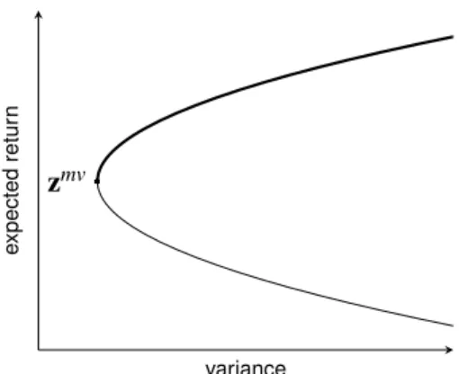
(5) is obtained. With a, c and f defined as in (5), and the determinant D = a f − cc of the 2 × 2 matrix positive as in Merton (1972), the minimum-variance frontier of (4) is the parabola

z

= 1

D ( f z

− 2cz

+ a)

Such a parabola is given in Figure 1. The minimum-variance point on the parabola z

and its corresponding portfolio x

in decision space are given by

z

= ( 1 f , c

f ) x

= 1 f Σ

1

In (variance, expected return)-space, the nondominated frontier is the upper part of the parabola starting at z

. The set of all portfolios that are inverse images of points on the nondominated frontier constitutes the efficient set and is given by

{ x ∈ R

| x = x

+ λ (Σ

µ − c

f Σ

1), λ ≥ 0 } (6) Note that the efficient set of Merton (1972)(6) is an unbounded line segment ema- nating from x

.

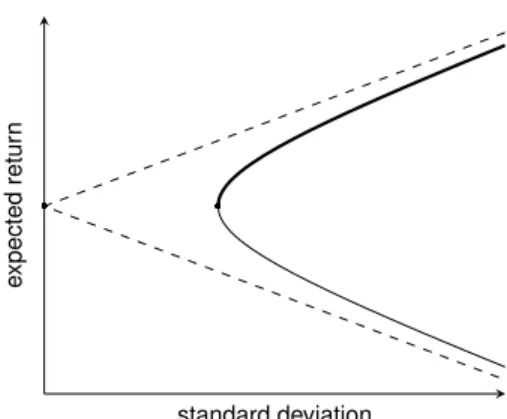
With it common to display the nondominated frontier in (standard deviation, expected return)-space, we have Figure 2. In this figure, because of the change from variance to standard deviation along the horizontal axis, the parabola becomes a hyperbola, with the upper part of the hyperbola starting at the minimum-standard deviation point now showing as the nondominated frontier. The dashed lines in the figure are the asymptotes of the hyperbola given by

z

= c f ±

s Dz

f for z

≥ 0 where √

z

is standard deviation.

Also covered in Merton (1972) is the 2-mutual-fund theorem. The theorem

is as follows. Let x

and x

be any two portfolios whose criterion vectors are on

z

variance

expectedreturn

Figure 1: A minimum-variance frontier plotted in (variance, expected return)- space where it is a parabola. The portion of the parabola from z

upward is the nondominated frontier in this space.

the minimum-variance (or minimum-standard deviation) frontier, and let x be any other portfolio (i.e., any vector in R

whose components sum to one). Then, the criterion vector of x is on the minimum-variance (or minimum-standard deviation) frontier iff x can be formed as a linear combination of x

and x

whose weights sum to one.

3 Deriving the minimum-variance surface

Following the literature with regard to the growing interest in additional criteria in portfolio selection, let us add an additional objective to (4) to form the following tri-criterion model

min { z

= x

Σx } (7)

max { z

= µ

x } max { z

= `

x }

s.t. 1

x = 1

While there are many candidates for a third criterion as discussed in Steuer et al. (2007), let us motivate our third criterion with portfolio liquidity, an arbitrary choice, for illustrative purposes. Hence, the `-vector in (7). As with the solution to model (4), the solution to (7) is all of its nondominated and efficient sets N and E . In analyzing (7), we make the following assumptions.

Assumption 1. Matrix Σ is positive definite.

standard deviation

expectedreturn

Figure 2: The same minimum-variance frontier plotted in (standard deviation, ex- pected return)-space where it is a hyperbola. The upper part of the hyperbola is the nondominated frontier in this space. The dashed lines are the asymptotes of the hyperbola.

Assumption 2. Vectors µ, ` and 1 are linearly independent.

Beginning as in the bi-criterion case, we form the following e-constraint repre- sentation of our tri-criterion model

min { z

=

x

Σ x } (8)

s.t. µ

x = z

`

x = z

1

x = 1

where z

and z

are arbitrary values of expected return and liquidity, respectively.

The union of all criterion vectors (z

, z

, z

) resulting from the optimal solutions of (8) for all values of z

and z

is the minimum-variance surface of (7). This is seen as a generalization of the minimum-variance frontier of (4). To begin the process of solving (8) for all values of z

and z

, we take the Lagrangian

L(x, g

,g

, g

) =

x

Σx + g

(z

− µ

x) + g

(z

− `

x) + g

(1 − 1

x)

where the g

are multipliers. Because x

Σ x is strictly convex by virtue of the

positive definiteness of Σ, L(x,g

, g

, g

) is strictly convex and x is the minimizing

solution of (8) iff

∂ L

∂ x = Σ x − g

µ − g

` − g

1 = 0

∂ L

∂ g

= z

− µ

x = 0

∂ L

∂ g

= z

− `

x = 0

∂ L

∂ g

= 1 − 1

x = 0

Premultiplying the first equation by Σ

enables us to obtain x = (g

Σ

µ +g

Σ

`+

g

Σ

1 ) . Substituting this into the last three equations of the above yields g

µ

Σ

µ + g

µ

Σ

` + g

µ

Σ

1 = z

g

µ

Σ

` + g

`

Σ

` + g

`

Σ

1 = z

g

µ

Σ

1 + g

`

Σ

1 + g

1

Σ

1 = 1

We introduce notation C and express the three equations above in matrix form as C



 g

g

g



 =



 z

z

1



 (9)

where

C =





µ

Σ

µ µ

Σ

` µ

Σ

1 µ

Σ

` `

Σ

` `

Σ

1 µ

Σ

1 `

Σ

1 1

Σ

1



 =





a b c

b d e

c e f





We now demonstrate the following property of C.

Lemma 1. Matrix C is positive definite.

Proof. Because Σ

is positive definite, it can function as a covariance matrix.

There exists a random vector v ∈ R

such that the covariance matrix of v is Σ

. In this way, C is the covariance matrix of the random vector

µ ` 1

v with C =

µ ` 1

Σ

µ ` 1

. Thus, for all y ∈ R

with y 6= 0, we have y

Cy = y

µ ` 1

Σ

µ ` 1

y. Define w =

µ ` 1

y. By Assumption 2, w 6=

0. Therefore, y

Cy = w

Σ

w > 0. Thus, C is positive definite.

By the positive definiteness of C, its determinant | C | > 0, and C

= 1

| C |





d f − ee ce − b f be − cd ce − b f a f − cc bc − ae be − cd bc − ae ad − bb





Premultiplying (9) by C

gives us



 g

g

g



 = C



 z

z

1



 = 1

| C |





z

( d f − ee ) + z

( ce − b f ) + ( be − cd ) z

(ce − b f ) + z

(a f − cc) + (bc − ae) z

(be − cd) + z

(bc − ae) + (ad − bb)





3×1

Substituting the above g

into the previously derived x = (g

Σ

µ + g

Σ

` + g

Σ

1 ) yields

x = 1

| C | [(z

(d f − ee) + z

(ce − b f ) + (be − cd))Σ

µ +(z

(ce − b f ) + z

(a f − cc) + (bc − ae))Σ

` +( z

( be − cd ) + z

( bc − ae ) + ( ad − bb ))Σ

1 ] or

x = x

+ z

d

+ z

d

(10)

where

x

= 1

| C | [(be − cd )Σ

µ + (bc − ae)Σ

` + (ad − bb)Σ

1 ] (11) d

= 1

| C | [( d f − ee )Σ

µ + ( ce − b f )Σ

` + ( be − cd )Σ

1 ] (12) d

= 1

| C | [(ce − b f )Σ

µ + (a f − cc)Σ

` + (bc − ae)Σ

1] (13) We interpret x

as the minimizing solution of (8) when z

= 0 and z

= 0. In this way,

{ x ∈ R

| x = x

+ z

d

+ z

d

, z

, z

∈ R } (14) is the set of all optimal solutions of (8) for all values of z

and z

, with the three vectors on the right in the set having the following property.

Lemma 2. Vectors x

, d

and d

are linearly independent.

Proof. Letting h

,h

, h

∈ R, by (11)-(13), we have h

x

+ h

d

+ h

d

= h

| C | [(be − cd)Σ

µ + (bc − ae)Σ

` + (ad − bb)Σ

1]

+ h

| C | [(d f − ee)Σ

µ + (ce − b f )Σ

` + (be − cd)Σ

1 ] + h

| C | [(ce − b f )Σ

µ + (a f − cc)Σ

` + (bc − ae)Σ

1]

After rearrangement, we have h

x

+ h

d

+ h

d

= 1

| C | {[(d f − ee)h

+ (ce − b f )h

+ (be − cd)h

]Σ

µ + [(ce − b f )h

+ (a f − cc)h

+ (bc − ae)h

]Σ

` + [(be − cd)h

+ (bc − ae)h

+ (ad − bb)h

]Σ

1 } By Assumptions 1 and 2, Σ

µ , Σ

` and Σ

1 are linearly independent. There- fore, the necessary and sufficient condition of h

x

+ h

d

+ h

d

= 0 is

(d f − ee)h

+ (ce − b f )h

+ (be − cd)h

= 0 (ce − b f )h

+ (a f − cc)h

+ (bc − ae)h

= 0 (be − cd )h

+ (bc − ae)h

+ (ad − bb)h

= 0

With the above reducing to C



 h

h

h



 = 0, and C

nonsingular, the only pos- sibility is that h

= h

= h

= 0. Therefore, x

, d

and d

are linearly indepen- dent.

With (14) being the set of all portfolios that generate the minimum-variance surface, it is seen that (14) is an affine set, in particular, being a 2-dimensional hyperplane in R

offset from the origin by x

. From this, as an extension of the 2- mutual-fund theorem of bi-criterion portfolio selection mentioned in Section 2, we can state the following 3-mutual-fund theorem of tri-criterion portfolio selection.

Theorem 1. Let x

, x

and x

be any three affinely independent

points from (14).

Then, any portfolio that generates a point on the minimum-variance surface can be formed by some linear combination of x

, x

and x

whose weights sum to one.

1Pointsx⁰,x¹,. . .,x^mare affinely independent ifx¹−x⁰,. . .,x^m−x⁰are linearly independent.

In criterion space, the minimum-variance surface of model (7) is obtained by substituting (10) into z

= x

Σ x to yield

z

= d

Σd

z

+ 2d

Σd

z

z

+ d

Σd

z

+ 2d

Σx

z

+ 2d

Σx

z

+ x

Σx

(15) where the six coefficients of (15) are specified in detail as

d

Σd

= 1

| C |

( ad

f

− 2ade

f + ae

− b

d f

+ b

e

f + 2bcde f − 2bce

− c

d

f + c

de

) d

Σd

= 1

|C|

(− abd f

+ abe

f + acde f − ace

+ b

f

+ bc

d f − 3b

ce f + 2bc

e

− c

de ) d

Σd

= 1

|C|

( a

d f

− a

e

f − ab

f

+ 2abce f − 2ac

d f + ac

e

+ b

c

f − 2bc

e + c

d ) d

Σ x

= 1

| C |

( abde f − abe

− acd

f + acde

− b

e f + b

cd f + 2b

ce

− 3bc

de + c

d

) d

Σ x

= 1

| C |

(−a

de f + a

e

+ ab

e f + abcd f − 3abce

+ ac

de − b

c f + 2b

c

e− bc

d ) x

Σ x

= 1

| C |

( a

d

f −a

de

− 2ab

d f + ab

e

+ 2abcde − ac

d

−2b

ce + b

f + b

c

d ) Let us now comment on the notion of an elliptic paraboloid. In (z

, z

, z

)-space, the expression z

= α

z

+ α

z

, where α

≥ 0 and α

≥ 0, is an elliptic paraboloid in standard form. The paraboloid is non-degenerate, if both α

> 0 and α

> 0.

Otherwise the paraboloid is degenerate. For a given value ζ > 0 of z

, we obtain

α2

ζ

z

+

ζ

z

= 1 in ( z

, z

) -space. This is recognized as an ellipsoid.

Theorem 2. The minimum-variance surface (15) of the tri-criterion portfolio prob- lem of (7) is a non-degenerate elliptic paraboloid.

Proof. We rewrite (15) as

z

=

z

z

1 P



 z

z

1



 where P =







d

Σ d

d

Σ d

d

Σ x

d

Σd

d

Σd

d

Σx

d

Σx

d

Σx

x

Σx





 . As Σ is a covariance matrix, let r ∈ R

designate the random vector associated with it. Form a new random vector

d

d

x

r. Let P be its covariance matrix.

For all y ∈ R

with y 6= 0, y

Py = y

d

d

x

Σ

d

d

x

y. Let w = d

d

x

y and w 6= 0 by Lemma 2. Then y

Py = w

Σ w > 0, because Σ is

positive definite. Therefore, P is positive definite.

With P positive definite, all of its eigenvalues v

, v

and v

are positive. With P real and symmetric, there exists a normal matrix N such that P = N





v

0 0 0 v

0 0 0 v



 N.

Hence, the minimum-variance surface (15) is z

=

z

z

1 N





v

0 0 0 v

0 0 0 v



 N



 z

z

1



 . Let u = N



 z

z

1



 . Then, z

= u





v

0 0 0 v

0 0 0 v



 u = v

u

+ v

u

+ v

u

. With v

, v

,v

>

0, after a change of coordinate system, we see the paraboloid as non-degenerate.

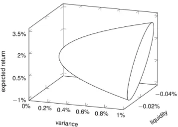
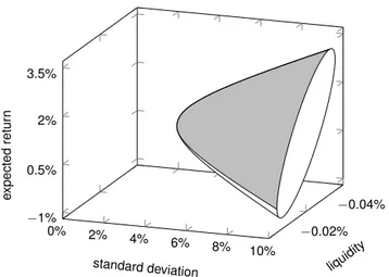
A depiction of a minimum-variance surface is given in Figure 3. The task of specifying the portion of the paraboloid that is the nondominated set of our tri- criterion model (7) still awaits us.

4 Deriving the nondominated surface

In order to compute the efficient and nondominated sets of model (7), we utilize a weighted-sums approach to form

min {

x

Σ x − λ

µ

x − λ

`

x } λ

, λ

≥ 0 (16) s.t. 1

x = 1

whose Langrangian is

L(x,g) =

x

Σx − λ

µ

x − λ

`

x + g(1 − 1

x)

where g is its multiplier. Because x

Σx is strictly convex, L(x, g) is strictly convex and x is the minimizing solution to (16) if and only if it satisfies

∂ L

∂ x = Σ x − λ

µ − λ

` − g1 = 0

∂ L

∂ g = 1 − 1

x = 0

Premultiplying the first equation by Σ

yields x = λ

Σ

µ + λ

Σ

` + gΣ

1.

Substituting x into the second equation produces

g = 1

1

Σ

1 (1 − λ

1

Σ

µ − λ

1

Σ

`) = 1

f (1 − λ

c − λ

e)

Noting that f > 0, the above is well-defined. Substituting g into x = (λ

Σ

µ + λ

Σ

` + gΣ

1 ) yields

x = λ

Σ

µ + λ

Σ

` + 1

f ( 1 − λ

c − λ

e )Σ

1 or

x = x

+ λ

∆

+ λ

∆

(17) where

x

= 1

f Σ

1 (18)

∆

= Σ

µ − c

f Σ

1 (19)

∆

= Σ

` − e

f Σ

1 (20)

Notice that the expression for x

, the minimum-variance portfolio, is the same for both Merton’s model (4) and the tri-criterion model (7) of this paper. The efficient set of (7) can then be expressed as

{ x ∈ R

| x = x

+ λ

∆

+ λ

∆

, λ

, λ

≥ 0 } (21) Lemma 3. Vectors ∆

and ∆

are linearly independent.

Proof. For h

, h

∈ R we have

h

∆

+ h

∆

= h

(Σ

µ − c

f Σ

1 ) + h

(Σ

` − e f Σ

1 )

= h

Σ

µ + h

Σ

` − ch

+ eh

f Σ

1 (22)

Since Σ

µ , Σ

` and Σ

1 are linearly independent, the right-hand side of (22) is zero iff h

= h

= 0, and −

= 0. Since only h

and h

are needed, ∆

and

∆

are linearly independent.

Therefore, generated by ∆

and ∆

, E is a translated 2-dimensional cone. Fur- thermore, note that the ∆

generator of (21) is the same as the single generator of (6). This means that any portfolio efficient in model (4) is efficient in model (7), and this immediately enables us to state the following theorem.

Theorem 3. The efficient set (6) of the bi-criterion model (4) is a subset of the

efficient set (21) of the tri-criterion model (7).

Thus by adding a linear criterion, the investor’s efficient set becomes a superset of its former self. By substituting (17) into model (7) we are able to demonstrate, as a function of λ

, λ

≥ 0, the nondominated set of (7) in the form of the following set of parametric equations

z

= (x

+ λ

∆

+ λ

∆

)

Σ(x

+ λ

∆

+ λ

∆

) z

= µ

( x

+ λ

∆

+ λ

∆

)

z

= `

( x

+ λ

∆

+ λ

∆

)

Whereas the nondominated set of Merton’s bi-criterion model (4) is a portion of the parabolic minimum-variance frontier (2), the nondominated set of the tri-criterion model is a portion of the paraboloidic minimum-variance surface (15).

5 Illustrative numerical example

We now provide a numerical example along with graphs to illustrate the results of this paper. To equip the example, data from the Center for Research in Secu- rity Prices (CRSP) were obtained over the period January 2009 to December 2013 on four stocks chosen from the Dow Jones Industrial Average index: American Express (AXP), Disney (DIS), Johnson & Johnson (JNJ), and Coca Cola (KO).

Monthly data over the period were downloaded for the covariance matrix Σ and the individual security expected return vector µ of model (7). Also, for the model’s liquidity vector `, we downloaded monthly closing bid, closing asked, and clos- ing prices so as to compute as our liquidity measure the negative of each stock’s bid-asked spread

closing price

. With all of this, we have

µ =







 0.0355 0.0240 0.0109 0.0135









` =









− 0.0003

− 0.0003

− 0.0002

− 0.0002







 Σ =









0.0182 0.0059 0.0016 0.0008 0.0059 0.0050 0.0014 0.0014 0.0016 0.0014 0.0018 0.0010 0.0008 0.0014 0.0010 0.0019







 (23) Utilizing the µ , ` and Σ of (23) in (11)–(13), we obtain

x

=









0.7643

− 2.7643 0.4959 2.5041









d

=









61.8479

− 61.8479

− 111.0574 111.0574









d

= 10

×









0.7553

− 1.7553

− 0.6975 1.6975









With these vectors inserted, in accordance with (14), the following set

{ x ∈ R

| x = x

+ z

d

+ z

d

, z

, z

∈ R }

−0.02%

−0.04%

0% 0.2% 0.4% 0.6% 0.8% 1%

−1%

0.5%

2%

3.5%

liquidity variance

expectedreturn

Figure 3: The portion of the paraboloidic minimum-variance surface of the illus- trative numerical example for variance z

≤ .01

gives the 2-dimensional hyperplane of portfolios in x-space that generates the minimum-variance surface. And by (15), we have

z

= 9.5778 × 10

z

+ 1.1396 × 10

z

z

+ 53.5843z

+ 242.7541z

+ 0.9582z

+ 0.0198 as the equation of the elliptic paraboloid that is the minimum-variance surface.

Graphing this, the minimum-variance surface is portrayed in Figure 3.

Now for the nondominated surface. Utilizing the µ, ` and Σ of (23) in (18)–

(20), we obtain

x

=









0.0158

− 0.0140 0.5210 0.4772









∆

=









0.8591 2.1633

− 3.5338 0.5114









∆

=









0.0028

− 0.0312 0.0137 0.0147









With these vectors inserted, in accordance with (17), the following set

{ x ∈ R

| x = x

+ λ

∆

+ λ

∆

, λ

, λ

≥ 0 } (24) gives the 2-dimensional translated cone of efficient portfolios in x-space that gener- ates the portion of the minimum-variance surface that is the nondominated surface.

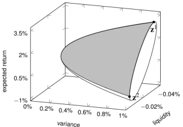
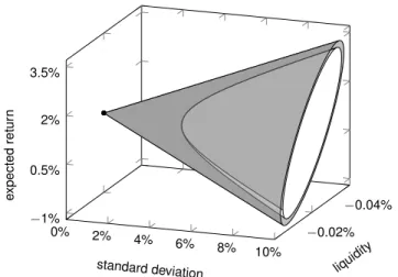
By substituting the vectors of the efficient set (24) into model (7), we obtain the nondominated surface as shown in gray in Figure 4.

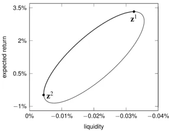
Notice the rightmost oval seen in Figure 4. It is the cross-section of the minimum-

variance surface with constant variance z

= 0.01. It is shown more directly in

−0.02%

−0.04%

0% 0.2% 0.4% 0.6% 0.8% 1%

−1%

0.5%

2%

3.5%

z

z

liquidity variance

expectedreturn

Figure 4: The portion of the minimum-variance surface that is the nondominated surface for variance z

≤ .01

Figure 5. As seen, the major axis of the ellipse is not parallel to either the z

or z

axis. Thus, the minimum-variance surface is rotated. This is a consequence of the fact that the d

Σd

coefficient of the z

z

term in the expression for the elliptic paraboloid above is not equal to 0. The heavier line between z

and z

inclusive is the portion of the ellipse that is nondominated.

As standard deviation is often more interpretable than variance (as standard de- viation is given in the same units as expected return), we now look at our plotting situation in terms of standard deviation. Whereas the parabola of Figure 1 becomes the hyperbola of Figure 2 when variance is changed to standard deviation in Mer- ton’s bi-criterion model (4), the paraboloid of Figure 3 becomes the hyperboloid seen in Figure 6 when variance is changed to standard deviation in our tri-criterion model (7).

Denoting standard deviation by z

= √

z

, the hyperboloid in given by z

=

q 9.5778 × 10

z

+ 1.1396 × 10

z

z

+ 53.5843z

+ 242.7541z

+ 0.9582z

+ 0.0198 While a hyperbola (as in Merton’s model) is surrounded by only 2 asymptotes, a

hyperboloid is surrounded by an asymptotic cone. Such an asymptotic cone can

be obtained by shifting the vertex of the paraboloid that corresponds to the hy-

perboloid in the z

direction to z

= 0. Since the vertex of the minimum-variance

paraboloid is the minimum-variance point, this involves a shift of z

=

= 1.4206 ×

−0.04%

−0.03%

−0.02%

−0.01%

0%

−1%

0.5%

2%

3.5%

z

z

liquidity

expectedreturn

Figure 5: Cross-section taken at variance z

= .01 showing the rotated nature of the minimum-variance surface

10

in our example. Thus, the asymptotic cone is given by q (z

)

+ 1.4206 × 10

=

q 9.5778 × 10

z

+ 1.1396 × 10

z

z

+ 53.5843z

+ 242.7541z

+ 0.9582z

+ 0.0198 or equivalently

(z

)

= 9.5778 × 10

z

+ 1.1396 × 10

z

z

+ 53.5843z

+ 242.7541z

+ 0.9582z

+ 0.0184 How the asymptotic cone encloses the hyperboloidic minimum-standard deviation

surface and nondominated surface is shown in Figure 7. The dot in the liquidity, expected return plane is the origin of the cone. This ends our illustrative example.

Acknowledgements

The authors are thankful to Markus Hirschberger for comments and to the software package PGFPLOTS by Feuers¨aanger (2014) for use in constructing the graphs.

The first author acknowledges support from the Ministry of Education of China

(Grant No. 14JJD630007), the National Natural Science Foundation of China

(Grant No. 71132001), and the Program for Changjiang Scholars and Innovative

Research Team in University, IRT0926.

−0.02%

−0.04%

0% 2% 4% 6% 8% 10%

−1%

0.5%

2%

3.5%

liquidity standard deviation

expectedreturn

Figure 6: The portions of the hyperboloidic minimum-standard deviation surface and nondominated surface of the illustrative numerical example for standard devi- ation √

z

≤ .10

References

[1] B. Aouni, C. Colapinto, and D. La Torre. Financial portfolio management through the goal programming model: Current state-of-the-art. European Journal of Operational Research, 234(2):536–545, 2015.

[2] Enrique Ballestero, Mila Bravo, Blanca P´erez-Gladish, Mar Arenas-Parra, and David Pl`a-Santamaria. Socially responsible investment: A multicriteria approach to portfolio selection combining ethical and financial objectives.

European Journal of Operational Research, 216(2):487–494, 2012.

[3] Carlos A. Bana e Costa and Jo˜ao O. Soares. Multicriteria approaches for portfolio selection: An overview. Review of Financial Markets, 4(1):19–26, 2001.

[4] Fouad Ben Abdelaziz, Belaid Aouni, and Rimeh El Fayedh. Multi-objective stochastic programming for portfolio selection. European Journal of Opera- tional Research, 177(3):1811–1823, 2007.

[5] A. Bilbao-Terol, M. Arenas-Parra, V. Ca˜nal-Fern´andez, and C. Bilbao-Terol.

Selection of socially responsible portfolios using hedonic prices. Journal of

Business Ethics, 115:515–529, 2013.

−0.02%

−0.04%

0% 2% 4% 6% 8% 10%

−1%

0.5%

2%

3.5%

liquidity standard deviation

expectedreturn

Figure 7: Figure 6 with enclosing asymptotic cone for standard deviation √

z

≤ .10 [6] J. M. Cabello, F. Ruiz, Blanca P´erez-Gladish, and P. M´endez-Rodriguez.

Synthetic indicators of mutual funds’ environmental responsibility: An ap- plication of the reference point method. European Journal of Operational Research, 236(1):313–325, 2014.

[7] C. Calvo, C. Ivorra, and V. Liern. Fuzzy portfolio selection with non-financial goals: Exploring the efficient frontier. Annals of Operations Research, 2014.

[8] George Chow. Portfolio selection based on return, risk, and relative perfor- mance. Financial Analysts Journal, (March-April):54–60, 1995.

[9] Gregor Dorfleitner, Michaela Leidl, and Johannes Reeder. Theory of social returns in portfolio choice with application to microfinance. Journal of Asset Management, 13(6):384–400, 2012.

[10] Matthais Ehrgott. Multicriteria Optimization. Springer, 2nd edition, 2005.

[11] Matthias Ehrgott, Kathrin Klamroth, and Christian Schwehm. An MCDM ap- proach to portfolio optimization. European Journal of Operational Research, 155(3):752–770, 2004.

[12] C. Feuers¨anger. Manual for package PGFPLOTS. Version 1.11, Universit¨at Bonn., 2014.

[13] John B. Guerard and Andrew Mark. Data show importance of company R&D

in picking stocks. Pensions & Investments, 32(25):30–31, 2004.

[14] W. G. Hallerbach, H. Ning, A. Soppe, and J. Spronk. A framework for man- aging a portfolio of socially responsible investments. European Journal of Operational Research, 153(2):517–529, 2004.

[15] Markus Hirschberger, Ralph E. Steuer, Sebastian Utz, Maximilian Wimmer, and Yue Qi. Computing the nondominated surface in tri-criterion portfolio selection. Operations Research, 61(1):169–183, 2013.

[16] Chi-fu Huang and Robert H. Litzenberger. Foundations for Financial Eco- nomics. Prentice Hall, Englewood Cliffs, New Jersey, 1988.

[17] H. Konno and K.-I. Suzuki. A mean-variance-skewness portfolio optimiza- tion model. Journal of the Operations Research Society of Japan, 38(2):173–

187, 1995.

[18] S. M. Lee. Goal Programming for Decision Analysis. Auerbach Publishers, Philadelphia, 1972.

[19] Andrew W. Lo, Constantin Petrov, and Martin Wierzbicki. It’s 11pm – Do you know where your liquidity is? The mean-variance-liquidity frontier.

Journal of Investment Management, 1(1):55–93, 2003.

[20] Harry M. Markowitz. Portfolio selection. Journal of Finance, 7(1):77–91, 1952.

[21] Robert C. Merton. An analytical derivation of the efficient portfolio frontier.

Journal of Financial and Quantitative Analysis, 7(4):1851–1872, 1972.

[22] K. Miettinen. Nonlinear Multiobjective Optimization. Kluwer Academic Publishers, Boston, 1999.

[23] B. P´erez-Gladish, P. M´endez-Rodriguez, B. M’Zali, and P. Lang. Mutual funds efficiency measurement under financial and social responsibility crite- ria. Journal of Multi-Criteria Decision Analysis, 20(3-4):109–125, 2013.

[24] M. G. Speranza. A heuristic algorithm for a portfolio optimization model applied to the Milan stock market. Computers & Operations Research, 23(5):431–441, 1996.

[25] Jaap Spronk and Winfried G. Hallerbach. Financial modelling: Where to

go? With an illustration for portfolio management. European Journal of

Operational Research, 99(1):113–127, 1997.

[26] Jaap Spronk and G. M. Zambruno. A multiple-criteria approach to portfolio selection. In H. G¨oppl and R. Henn, editors, Geld, Banken und Versicherun- gen, pages 451–459. Band 1, Athenum, 1981.

[27] Ralph E. Steuer and P. Na. Multiple criteria decision making combined with finance: A categorized bibliography. European Journal of Operational Re- search, 150(3):496–515, 2003.

[28] Ralph E. Steuer, Yue Qi, and Markus Hirschberger. Suitable-portfolio in- vestors, nondominated frontier sensitivity, and the effect of multiple ob- jectives on standard portfolio selection. Annals of Operations Research, 152(1):297–317, 2007.

[29] B. K. Stone. A linear programming formulation of the general portfolio selec- tion problem. Journal of Financial and Quantitative Analysis, 8(4):621–636, 1973.

[30] Sebastian Utz, Maximilian Wimmer, Markus Hirschberger, and Ralph E.

Steuer. Tri-criterion inverse portfolio optimization with application to so- cially responsible mutual funds. European Journal of Operational Research, 234(2):491–498, 2014.

[31] Sebastian Utz, Maximilian Wimmer, and Ralph E. Steuer. Tri-criterion mod- eling for creating more-sustainable mutual funds. European Journal of Op- erational Research, 2015.

[32] Panos Xidonas, George Mavrotas, Theodore Krintas, John Psarras, and Con- stantin Zopounidis. Multicriteria Portfolio Management. Springer Verlag, Berlin, 2012.

[33] William T. Ziemba. Personal communication at 21st European Conference

on Operations Research, Reykjavik, Iceland, July 3, 2006.