Quantifying the time lag between organic matter production and export in the surface ocean: Implications for
estimates of export ef fi ciency
P. Stange1 , L. T. Bach1 , F. A. C. Le Moigne1 , J. Taucher1 , T. Boxhammer1 , and U. Riebesell1
1GEOMAR Helmholtz Centre for Ocean Research Kiel, Kiel, Germany
Abstract
The ocean’s potential to export carbon to depth partly depends on the fraction of primary production (PP) sinking out of the euphotic zone (i.e., thee-ratio). Measurements of PP and exportflux are often performed simultaneously in thefield, although there is a temporal delay between those parameters.Thus, resultinge-ratio estimates often incorrectly assume an instantaneous downward export of PP to exportflux. Evaluating results from four mesocosm studies, wefind that peaks in organic matter
sedimentation lag chlorophyllapeaks by 2 to 15 days. We discuss the implications of these time lags (TLs) for currente-ratio estimates and evaluate potential controls of TL. Our analysis reveals a strong correlation between TL and the duration of chlorophyllabuildup, indicating a dependency of TL on plankton food web dynamics. This study is one step further toward time-correctede-ratio estimates.
1. Introduction
About 50 Pg of carbon arefixed into organic matter (OM) by marine phytoplankton in the surface ocean every year [Field, 1998]. The majority of this OM is rapidly remineralized in the surface ocean, and only 5 to 12 Pg C per year are exported out of the euphotic zone [Siegel et al., 2016], mainly in the form of sink- ing particles. The fraction of OM leaving the euphotic zone is increased by several processes, such as phy- sically and biotically mediated particle aggregation [Burd and Jackson, 2009], as well as scavenging of ballasting minerals [Armstrong et al., 2002;Francois et al., 2002;Klaas and Archer, 2002]. However, particle reprocessing usually lasts hours to days. Thus, sinking OM reaches the bottom of the euphotic zone
“long” after its formation in the surface and may take much longer to eventually reach the seafloor [Deuser, 1986]. Quantifying this time lag (TL) is challenging, as it requires tracing of OM from its produc- tion in the surface to the collection at depth.
Using outputs from a global biogeochemical model,Henson et al. [2015] recently calculated that the TL varies substantially throughout the oceans, with generally longer TLs at high compared to low latitudes. This varia- bility was attributed to differences in seasonality. High latitudes are characterized by pulsed biomass forma- tion during spring and late summer, commonly driven by large phytoplankton such as diatoms [Martin et al., 2011]. The time it takes for single cells to aggregate into sinking particles results in delayed exportfluxes. This delay can be intensified by a mismatch between phytoplankton and zooplankton due to the lag of repacka- ging into fecal pellets [Lam and Bishop, 2007;Lam et al., 2011]. In contrast, at low latitudes shorter TLs may result from more constant primary production throughout the year and a tighter coupling between phyto- plankton production and zooplankton grazing [Henson et al., 2015].
Due to the scarcity of available time series data in large parts of the ocean, exportflux and primary production (PP) are commonly measured during ship-based expeditions. However, due to logistic constraints these mea- surements are often conducted simultaneously, neglecting lateral advection and TL and thereby connecting PP values to collected organic matter that may have a different origin (Figure 1).
PP is commonly measured using14C or18O incubations [Nielsen, 1952;Bender et al., 1987], fast repetition rate fluorometry, or O2:Ar ratios [Kolber and Falkowski, 1992;Kolber et al., 1998;Martin et al., 2013]; all of which inte- grate over very short time scales of a few hours to 1 day. Exportflux, however, is either directly measured with sediment traps or marine snow catchers [Knauer et al., 1979;Riley et al., 2012] or estimated from particle reac- tive radionuclides (e.g.,234Th and210Po) [Buesseler et al., 1992;Cochran and Masqué, 2003;Le Moigne et al., 2013a]. These measurements integrate exportflux over a few hours up to months [Le Moigne et al., 2013b].
PUBLICATIONS
Geophysical Research Letters
RESEARCH LETTER
10.1002/2016GL070875
Key Points:
•We calculated time lags between peaks in chlorophyll a and organic matter sedimentation for four mesocosm studies in different regions
•Time lags varied between 2 to 15 days at the surface and increased with depth depending on sinking velocities
•Time lag correlated with chlorophylla buildup rate, indicating a dependency of time lag on the plankton community structure
Supporting Information:
•Table S1
Correspondence to:
P. Stange, pstange@geomar.de
Citation:
Stange, P., L. T. Bach, F. A. C. Le Moigne, J. Taucher, T. Boxhammer, and U. Riebesell (2016), Quantifying the time lag between organic matter production and export in the surface ocean:
Implications for estimates of export efficiency,Geophys. Res. Lett.,43, doi:10.1002/2016GL070875.
Received 17 AUG 2016 Accepted 16 DEC 2016
Accepted article online 17 DEC 2016
©2016. The Authors.
This is an open access article under the terms of the Creative Commons Attribution-NonCommercial-NoDerivs License, which permits use and distri- bution in any medium, provided the original work is properly cited, the use is non-commercial and no modifications or adaptations are made.
Suchin situmeasurements of PP and exportflux are subsequently used to estimate the efficiency with which organic carbon is exported from the euphotic zone, also referred to as export- ore-ratio:
e-ratio¼export flux
PP (1)
Thee-ratio is thus based on the assumption that the material collected at depth originates from the mea- sured surface PP. However, this is not necessarily the case when measurements are done simultaneously and integration time scales are insufficiently long (Figure 1). Accordingly, impossiblee-ratio estimates greater than 1 [Le Moigne et al., 2015] are commonly observed when neglecting TL. Lateral advection of organic mat- ter is another factor that should also be taken into account but is not addressed in this study. Thee-ratios will only provide the actual export efficiency of a system if the OM collected at export depth is traced back to the surface PP it originates from.
In this study we evaluated water column chlorophyllaconcentrations and sedimentation of organic matter over time from fourin situmesocosm studies [Riebesell et al., 2013] conducted in arctic (Kongsfjord, Svalbard), temperate (Gullmar Fjord, Sweden and Raunefjord, Norway), and subtropical regions (Gando Bay, Gran Canaria). We aimed to quantify the time it takes from peak surface production to peak sedimentation of sink- ing particles. Further, we assess potential controls that may drive differences in TL among the different study sites.
2. Methods
2.1. Experimental Design
In order to quantify TL we used the results of four mesocosm campaigns conducted between 2010 and 2014.
All of these experiments focused on the effects of ocean acidification on plankton communities; however, we only included untreated (control) mesocosms in the analysis here. The four studies were conducted in Kongsfjord (Svalbard; 78.93667°N, 11.89333°E), Raunefjord (Norway; 60.265°N, 5.205°E), Gullmar Fjord Figure 1.Conceptualfigure illustrating the problem of in situ estimation of the export efficiency. Exportflux is commonly correlated with simultaneous measurements of primary production (PP2), which delivers incorrecte-ratio estimates (red).
In order to correctly estimate the export efficiency of the system, collected material at depth has to be related to the primary production measurements conducted at the time of its production in the surface (PP1). Accuratee-ratio estimates (green) thus have to account for both the time lag (TL) between PP and organic matter collection at depth and lateral advection of the latter on its way through the water column. This study emphasizes the importance of TL ine-ratio estimates and shows its range over different study sites.
(Sweden; 58.26635°N, 11.47832°E), and Gando Bay (Gran Canaria, Spain; 27.92798°N, 15.36540°W). Further information on each experiment is given in Table S1 in the supporting information, and detailed descriptions regarding the experimental design are provided bySchulz et al. [2013] and Bach et al. [2016a, 2016b].
Experiments are henceforth referred to as SB2010, N2011, S2013, and GC2014as specified in Table S1.
The Kiel Off-Shore Mesocosms for Future Ocean Simulations (KOSMOS) were used in all of the experiments, which consist of a cylindrical polyurethane bag mounted in an 8 m longflotation frame [Riebesell et al., 2013].
The bag ends in a 2 m long conical sediment trap with a collection cylinder attached to it [Boxhammer et al., 2016]. The bottom of the cylinder is connected to the sea surface via a silicon tube that is used for vacuum sampling of sedimented matter. The sediment trap attachment to the mesocosm bags has been modified between SB2010and N2011, which did, however, not influence the trapping efficiency [Riebesell et al., 2013].
Mesocosm lengths differed between experiments, ranging from 25 m in N2011to 15 m in GC2014(Table S1).
Mesocosms were deployed following a similar protocol in each experiment as described bySchulz et al.
[2013]. Temperature was measured with a hand-operated conductivity-temperature-depth (Sea and Sun Technology). Depth- and time-averaged temperatures for each campaign are given in Table S1.
2.2. Analysis of Surface Production
Samples for phytoplankton chlorophylla(Chla) analysis were taken every day (N2011) or every other day (SB2010, S2013, and GC2014) with an integrating water sampler (HydroBios), which automatically collects equal amounts of volume at each depth. Chlasamples werefiltered on GF/Ffilters and immediately frozen at80°C (described in detail byPaul et al. [2015]). Chlaconcentrations were determined by reverse-phase high- performance liquid chromatography (HPLC). Filters from SB2010and N2011were analyzed using a WATERS HPLC with a Varian Microsorb-MV 100-3 C8 column [Barlow et al., 1997], whilefilters from S2013and GC2014were analyzed with a Thermo Scientific HPLC Ultimate 3000 with an Eclipse XDB-C8 3.5 u 4.6 × 150 column [Van Heukelem and Thomas, 2001].
2.3. Sedimenting Organic Matter
Sediment trap samples were collected every other day, except for N2011, where sampling was conducted daily following the methodology detailed inBoxhammer et al. [2016]. Briefly, samples were vacuum-pumped to the sea surface through a tube reaching down to the bottom of the collection cylinder of the sediment trap. The dense particle suspension was collected in 5 L glass bottles and transported unpoisoned to the land-based facilities within 1–3 h after collection. During GC2014, samples were stored in large coolers (Coleman) throughout the sampling procedure due to higher air temperatures and the somewhat longer time (4–5 h) until processing. Subsequently, particles were concentrated by passive settling (SB2010and N2011), precipitation with theflocculant FeCl3(S2013), or centrifugation (GC2014). All approaches yield compar- able results and are described byBoxhammer et al. [2016]. The resulting sediment pellets were stored at20°C, freeze-dried, ground for homogenization, and then analyzed for total particulate carbon (TPC) with an elemen- tal analyzer (Euro EA–CN, Hekatech) according to Sharp [Sharp, 1974]. Finally, TPC data were normalized by mesocosm volume.
2.4. Evaluation of Time Lag Between the Peaks of Chlaand OM Sedimentation
In order to quantify TL we identified the temporal difference of the peaks in water column Chla(PChl) and peaks in sedimented total carbon (PSed) and extrapolated to 100 m as described in the next section. Chlacon- centrations were used, as PP data were only available for two out of the four experiments and the low tem- poral resolution of these data did not allow for a precise determination of TL. C/Chl ratios did vary at the different locations, but Chl a concentrations were still the most reliable bloom indicator available.
Phytoplankton blooms were identified using the threshold method [Siegel et al., 2002;Brody et al., 2013].
Briefly, median Chlaconcentrations were calculated for each experiment and thefirst value equal to or above the median prior to the peak marks the bloom start date (BSD). The same method was applied to the sedimented total carbon concentrations to estimate massflux initiation. The time from BSD to the peak in Chlawas evaluated for each mesocosm of the respective experiments and is hereafter referred to as dura- tion of Chlabuildup. Note that we focused on inorganic nutrient-fueled phytoplankton blooms in this ana- lysis of mesocosm data as we could only detect Chlaand subsequent sinkingflux peaks in such settings. In later stages of the experiments OM production was often fueled by organic nutrients and resulted in smaller and more irregular pulses in OM sedimentation, thus making a precise assignment of peaks impossible.
Geophysical Research Letters
10.1002/2016GL0708752.5. Amplification of the Time Lag Between PP and Sinking Matter Flux With Depth
The range over which the time lag in the surface amplifies with depth primarily depends on how fast the organic matter sinks. Sinking velocity (SV) measurements were performed during each study except for the SB2010experiment using the FlowCam method [Bach et al., 2012]. Briefly, a subsample of bulk material collected in the sediment trap is transferred to a sinking chamber, which is mounted in a modified version of the FlowCam (Fluid Imaging). Settling particles are recorded for ~20 min atin situtemperature of the meso- cosms. This enables the characterization and tracking of individual particles in the size range of 40–400μm, except for the last study (GC2014), where we used a larger sinking chamber allowing for a larger particle size spectrum (40–1000μm). Using this method, we measured size and SV of particles each day sediment trap samples were collected. From these measurements we get a correlation of sinking velocity to particle dia- meter. We use this correlation to calculate the SV for any given particle diameter:
SV Nð 2011Þ ¼0:04754Dþ1:5465 (2)
SV Sð 2013Þ ¼0:054Dþ2:3 (3)
SV GC2014ð Þ ¼0:07706Dþ21:15572 (4)
where SV is the particle sinking velocity in m d1andDis the particle diameter inμm (equation (3) adopted fromEnke[2014]). Using these equations, we then calculated the average SV of the particle size spectrum (100–1000μm), which covers the size spectrum of particles responsible for the majority of massflux [Clegg and Whitfield, 1990]. Several processes have been reported to influence the sinking velocity of particles both negatively and positively. Processes that accelerate particle sinking involve, e.g., bacterial remineralization, scavenging of ballasting minerals, and repackaging by grazers [Armstrong et al., 2002;Francois et al., 2002;
Klaas and Archer, 2002;Turner, 2002;Ploug et al., 2008], while other processes decelerate particle sinking to depth, e.g., sinking through density gradients [MacIntyre et al., 1995;Prairie et al., 2013]. For our extrapolation of TL to 100 m we assumed a range of slow- to fast-sinking velocities based on the size versus sinking velocity relationship from the individual study sites (see above). It is important to note that we did not explicitly con- sider the variability of SV that is introduced through nonsize-related factors (e.g., ballast) in this extrapolation.
However, we are confident that the uncertainty in SV generated through nonsize-related parameters is smal- ler than the range covered by the wide size spectrum. This confidence is based on observations in a previous study where maximum changes in SV due to changing excess density were within 30–40% of the total var- iance within a period of 4 weeks [Bach et al., 2016b].
We hereafter differentiate between the initial time lag (TL; time lag between peak Chlaand peak sedimenta- tion of total carbon in the mesocosms) and the time lag at 100 m depth (TL100; time lag betweenPChland the point in time when sinking OM reaches 100 m water depth).
3. Results and Discussion
3.1. Observations of Time Lag Between Phytoplankton Blooms and Sedimentation From Several Mesocosm Studies
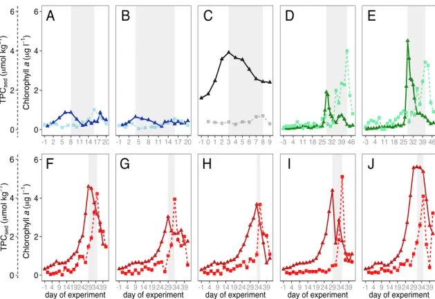
Table S1 lists the TL calculated for each mesocosm and location, as well as the concentrations of Chlaand TPC atPChlandPSed, respectively. Temporal development of Chlaconcentrations and sedimentation of TPC are shown for each mesocosm in Figure 2. TLs varied between locations, ranging from 2 to 15 days, and to a lesser extent between replicate mesocosms (see Figure 3a). Error bars indicate the uncertainty asso- ciated with the identification of peaks in days, as Chlaconcentrations and sedimentation were not measured on a daily basis in all experiments.
In the SB2010experiment, Chlaconcentration peaked at days 8 (Figure 2a) and 4 (Figure 2b) with 0.87 and 0.65μg L1, which led to a sedimentation of 1.01 and 0.54μmol kg148 h1TPC at day 16. Chlabuildup took 4 (M3) or 2 (M7) days. This experiment was characterized by comparatively long TLs of 8 (2) and 12 (2) days.
The N2011experiment showed high peak Chlaconcentrations of 3.92μg L1at day 3 (Figure 2c). Using the threshold method, we determined that Chlabuilt up over 1 day, which does not reflect the observed data.
This discrepancy results from the fact that Chlaconcentrations stayed high after thePChland did not return to low values as observed in the other experiments. This leads to relatively high median Chlaconcentration, which in turn is used to determine the BSD. However, this discrepancy between observed and calculated
BSDs was only an issue for this particular mesocosm. For the other locations, the calculated BSD agreed well with the observations. Sedimentation of OM was rather low during N2011, with a peak of 0.7μmol kg1d1TPC on day 8. The observed TL during N2011was 5 days. There was no uncertainty associated with the daily determina- tion of TL during N2011, as both Chlaconcentrations and sedimentfluxes were determined every day.
In S2013(Figures 2f–2j), we observed the highest peak Chlaconcentrations (4.61 (M1), 3.03 (M3), 3.67 (M5), 4.40 (M9), and 5.62 (M10)μg L1) and sinkingfluxes (4.23, 3.94, 3.67, 5.11, and 4.1μmol kg148 h1TPC).
Although this study displayed some of the shortest TLs of all data sets (6, 4, 2, 6, and 42 days), Chla increased very slowly over 14 days. Due to the high number of replicates in this experiment (n= 5), we were able to get a better estimate of the variability of TL among replicates. We observed up to a threefold differ- ence in TL between replicate mesocosms.
During GC2014(Figures 2d and 2e), peak Chlaconcentrations were high (1.91 (M1) and 4.51 (M9)μg L1) and they increased more rapidly (2 and 3 days) compared to S2013. The sinkingflux in this experiment showed a slower increase despite peaks being high (3.99 and 3.42μmol kg148 h1TPC). We observed the longest TLs of 13 and 15 (1) days in this experiment.
To estimate the amplification of TL betweenPChlandPSedup to 100 m water depth (TL100; Figure 3b), we cal- culated average sinking velocities for N2011, S2013, and GC2014using equations (2)–(4), respectively. For a par- ticle size of 500μm, this resulted in sinking velocities of 25.3 m d1(N2011), 29.3 m d1(S2013), and 59.7 m d1 (GC2014), which is well within the range expected for this size (seeBach et al. [2016b] for a detailed discussion).
The considerably higher sinking velocities during GC2014can be explained by two mechanisms: (1) the supply of Saharan dust to the mesocosms was likely higher during GC2014compared to the other studies, both due to dust events commonly appearing during the period in which the GC2014study took place and likely due to additional supply of volcanic sand from the islands as the mesocosms were positioned ~100–200 m down- wind of a large headland. (2) Average water temperatures were higher during GC2014, leading to a decrease in water viscosity with potential to increase sinking velocity [Taucher et al., 2014].
Figure 2.Chlorophyllaconcentrations (solid lines) and organic matter concentrations (dashed lines), collected in the sediment traps during (a and b) SB2010, (c) N2011, (d and e) GC2014, and (f–j) S2013. The shaded areas indicate the time lag from Chlapeaks to sedimentation peaks. Note that OM concentrations are based on daily sampling for N2011and every other day sampling for SB2010, S2013, and GC2014. The colors differentiate the four sampling locations.
Geophysical Research Letters
10.1002/2016GL070875Due to higher sinking velocities in GC2014, the mean TL100(average of cal- culated TL100 for 100μm and 1000μm particle diameter) converges with those of the other experiments at depth. Thus, mean TL100ranges from 8 to 17 days (see Figure 3b). However, the spread of TLs increases with depth as a function of minimum and maximum sinking veloci- ties. Thus, locations with overall slower sinking velocities show a larger range at 100 m.
3.2. Importance of Time Lag ine-Ratio Estimates
This study revealed a relatively large range (2 to 15 days) in TL between sur- face production and particle collection in the sediment traps. TL amplifies with increasing depth depending on particle sinking velocities. At sea, measurements of PP and exportflux are commonly per- formed on the same day and used to cal- culate the export efficiency of a given system. However, without the considera- tion of TL, the measured export flux is not connected to the surface production it originates from. Thus, resultinge-ratio estimates do not reflect the true export efficiency of the system and are less reli- able the longer TL becomes (see Figure 1). This is likely to be more impor- tant in highly seasonal regions, such as the North Atlantic, the Arctic, and many coastal areas, where PP and export occur in a much more pulsed fashion relative to oligotrophic regions. In order to cor- rectly connect PP to exportflux, the OM produced in the surface would have to be traced and collected at depth.
Unfortunately, conventional approaches are unable to resolve this connection or are limited by the duration of studies.
An alternative would be (1) to extend and more importantly (2) to synchronize the integration time of primary produc- tion and export flux estimates. The for- mer has partly been implemented with the introduction of the ThEi ratio, in which the time scale of satellite-derived estimates of PP were adapted to match thorium-derived estimates of export flux [Henson et al., 2011; Le Moigne et al., 2016]. Although this approach is still limited by the half-life time of thorium (approximately 24 days), it includes a potential Figure 3.(a) Time lags in days betweenPChlandPSed(see section 2.4) of
all mesocosms from SB2010(M3 and M7; blue), N2011(M4; black), S2013 (M1, M3, M5, and M9; red), and GC2014(M1 and M9; green). The error bars indicate the uncertainty in days. (b) Amplification of time lag down to 100 m depth. SB2010is absent due to missing sinking velocity data.
Amplification of time lag for a range of particle sizes is indicated by shaded areas (upper limit = 100μm, lower limit = 1000μm, and line = mean). The colors represent the different experiments, and for ease of readability, only the mesocosms with longest and shortest TL were displayed (N2011(M4) = black, S2013(M1, M5) = red, and GC2014(M1, M9) = green).
(c) Correlation between TL and the duration of Chlabuildup. For the N2011study, Chlabuildup determined with the threshold method did not match the observation and was excluded from the analysis (black asterisk; see section 3.1).
time lag within this time frame. Our results suggest that the integration time of theThEimethod would be sufficient to account for both the TL and TL100. However, the large range of TL observed in our studies indi- cates that the amplification of TL at depth can occasionally exceed 1 month when TL is large and particle sink- ing velocities are low. Thus, the integration time of theThEiapproach may occasionally still be too small for accuratee-ratio estimations. It also has to be noted that this method does not account for lateral transport of sinking particulate matter, which remains an unsolved problem ine-ratio estimation in thefield.
3.3. What Are Potential Controls on the Time Lag Between PP and Sinking Particle Production?
Ultimately, the aim is to adequately estimate the export efficiency of a given system. Thus, sampling for both PP and exportflux have to integrate on adequate time scales or account for the TL. It is therefore crucial to identify and understand the underlying mechanisms that drive differences in this TL. In order tofind mechan- isms controlling the length of TL, we tested for potential correlations between TL and (1) duration of Chla buildup (bloom start to Chlapeak), (2) temperature, and (3) mesocosm length.
A strong positive correlation was found between TL and duration of Chl a buildup (y= 18.14e(0.15x), r2= 0.899,p<0.001,n= 9; Figure 3c). A possible explanation for this correlation could be a dependency of TL on the dynamics between primary producers and grazers in the system. A rapid Chlaincrease, as observed during the GC2014and SB2010experiments, leads to a stronger disequilibrium between primary producers and consumers. This may delay one of the major pathways of OM export, i.e., repackaging of phytoplankton OM into fecal pellets by grazers. This loss of the packaging function has previously been described as a poten- tial mechanism to control export of particles to the mesopelagic [Lam et al., 2011]. Contrastingly, in systems with slow biomass buildup (e.g., S2013), phytoplankton and grazer growth is likely to be more tightly coupled so that particle aggregation follows OM production with less delay. Indeed,Henson et al. [2015] reported long TLs at high-latitude regions characterized by pulsed surface production and short TLs in low-latitude regions characterized by more tightly coupled food webs.
The repackaging control on TL proposed above seems to be contradicted by the higher sinking speeds mea- sured during GC2014. However, as explained in section 3.1, we attribute these elevated sinking velocities to other factors (ballasting and low viscosity) so that this data set does not contradict the food web mechanism described above.
Another possible explanation for variable TLs could be that aggregation processes took longer in SB2010and GC2014due to differences in phytoplankton community composition. It has been shown that coagulation effi- ciency can vary substantially depending on phytoplankton species composition, nutritional status, and growth phase of the cells [Kiørboe et al., 1990; Kiørboe and Hansen, 1993; Burd and Jackson, 2009].
Unfortunately, we currently do not have enough understanding of the influence of these settings and their interaction on the rate of particle formation. Identifying which of these mechanisms (zooplankton repacka- ging or aggregation efficiency) is dominant in different plankton communities at specific times exceeds the scope of this study and will be addressed in future work.
We also found a weak positive correlation of TL and temperature (y= 0.038x+ 4.57,r2= 0.559, p= 0.013, n= 10). These results contradict thefinding ofHenson et al. [2015], who observed larger TLs at high latitudes than at lower ones. However, wefind a high variability in TLs even at the same temperature (average tem- perature in SB2010and S2013= 3°C; TL ranged between 2 and 12 days), suggesting that temperature may not be the controlling factor of the range in TL. A weak negative correlation was also found between TL and mesocosm length (y=0.97x+ 24.9,r2= 0.488,p= 0.025,n= 10) with longer TLs occurring in shorter mesocosms. This is counterintuitive and we conclude that this results from a coincidental co-correlation of length with food web structure rather than a true causal relation.
4. Conclusion
In this study we aimed to constrain the time lag between PP and exportflux in different oceanic regions. We observed a relatively large range in TL of 2 to 15 days. The longest TLs were found in systems characterized by rapid Chlaincreases. This illustrates that, when coupled with exportflux measurements, instantaneous mea- surements of PP are insufficient to adequately estimate the export ratio and longer time scales must be con- sidered. Our analysis further showed that the duration of TL correlates with the duration of Chlabuildup, indicating a strong coupling of TL with biological parameters, i.e., phytoplankton community composition
Geophysical Research Letters
10.1002/2016GL070875and/or food web dynamics. This study represents one step toward a time-correctede-ratio (e-ratioTC), which would portray a more accurate picture of differences in export efficiency among the ocean basins.
References
Armstrong, R. A., C. Lee, J. I. Hedges, S. Honjo, and S. G. Wakeham (2002), A new, mechanistic model for organic carbonfluxes in the ocean based on the quantitative association of POC with ballast minerals,Deep. Res. Part II Top. Stud. Oceanogr.,49, 219–236, doi:10.1016/S0967- 0645(01)00101-1.
Bach, L. T., U. Riebesell, S. Sett, S. Febiri, P. Rzepka, and K. G. Schulz (2012), An approach for particle sinking velocity measurements in the 3–400μm size range and considerations on the effect of temperature on sinking rates,Mar. Biol.,159(8), 1853–1864, doi:10.1007/s00227- 012-1945-2.
Bach, L. T., et al. (2016a), Influence of ocean acidification on a natural winter-to-summer plankton succession: First insights from a long-term mesocosm study draw attention to periods of low nutrient concentrations,PLoS One,11(8), e0159068, doi:10.1371/journal.pone.0159068.
Bach, L. T., T. Boxhammer, A. Larsen, N. Hildebrandt, K. G. Schulz, and U. Riebesell (2016b), Influence of plankton community structure on the sinking velocity of marine aggregates,Global Biogeochem. Cycles,30, 1145–1165, doi:10.1002/2016GB005372.
Barlow, R., D. Cummings, and S. Gibb (1997), Improved resolution of mono- and divinyl chlorophyllsaandband zeaxanthin and lutein in phytoplankton extracts using reverse phase C-8 HPLC,Mar. Ecol. Prog. Ser.,161, 303–307, doi:10.3354/meps161303.
Bender, M., et al. (1987), A comparison of four methods for determining planktonic community production 1,Limnol. Oceanogr.,32(5), 1085–1098, doi:10.4319/lo.1987.32.5.1085.
Boxhammer, T., L. T. Bach, J. Czerny, and U. Riebesell (2016), Technical note: Sampling and processing of mesocosm sediment trap material for quantitative biogeochemical analysis,Biogeosciences,13(9), 2849–2858, doi:10.5194/bg-13-2849-2016.
Brody, S. R., M. S. Lozier, and J. P. Dunne (2013), A comparison of methods to determine phytoplankton bloom initiation,J. Geophys. Res.
Ocean,118, 2345–2357, doi:10.1002/jgrc.20167.
Buesseler, K. O., M. P. Bacon, J. Kirk Cochran, and H. D. Livingston (1992), Carbon and nitrogen export during the JGOFS North Atlantic Bloom experiment estimated from234Th:238U disequilibria,Deep Sea Res. Part A. Oceanogr. Res. Pap.,39(7–8), 1115–1137, doi:10.1016/0198-0149 (92)90060-7.
Burd, A. B., and G. A. Jackson (2009), Particle aggregation,Annu. Rev. Mar. Sci.,1(1), 65–90, doi:10.1146/annurev.marine.010908.163904.
Clegg, S. L., and M. Whitfield (1990), A generalized model for the scavenging of trace metals in the open ocean—I. Particle cycling,Deep Sea Res. Part A. Oceanogr. Res. Pap.,37(5), 809–832, doi:10.1016/0198-0149(90)90008-J.
Cochran, J. K., and P. Masqué (2003), Short-lived U/Th series radionuclides in the ocean: tracers for scavenging rates, exportfluxes and particle dynamics,Rev. Mineral. Geochem.,52(1), 461–492, doi:10.2113/0520461.
Deuser, W. G. (1986), Seasonal and interannual variations in deep-water particlefluxes in the Sargasso Sea and their relation to surface hydrography,Deep Sea Res. Part A, Oceanogr. Res. Pap.,33(2), 225–246, doi:10.1016/0198-0149(86)90120-2.
Enke, G. (2014), Sinkingflux of particulate organic matter and the special role ofCoscinodiscus wailesii: A mesocosm experiment, Dresden Univ. of Technology, M.S. thesis, Dresden, Germany
Field, C. B. (1998), Primary production of the biosphere: Integrating terrestrial and oceanic components,Science,281(5374), 237–240, doi:10.1126/science.281.5374.237.
Francois, R., S. Honjo, R. Krishfield, and S. Manganini (2002), Factors controlling theflux of organic carbon to the bathypelagic zone of the ocean,Global Biogeochem. Cycles,16(4), 1087, doi:10.1029/2001GB001722.
Henson, S. A., R. Sanders, E. Madsen, P. J. Morris, F. Le Moigne, and G. D. Quartly (2011), A reduced estimate of the strength of the ocean’s biological carbon pump,Geophys. Res. Lett.,38, L04606, doi:10.1029/2011GL046735.
Henson, S. A., A. Yool, and R. Sanders (2015), Variability in efficiency of particulate organic carbon export: A model study,Global Biogeochem.
Cycles,29, 33–45, doi:10.1002/2014GB004965.
Kiørboe, T., and J. L. S. Hansen (1993), Phytoplankton aggregate formation: Observations of patterns and mechanisms of cell sticking and the significance of exopolymeric material,J. Plankton Res.,15(9), 993–1018, doi:10.1093/plankt/15.9.993.
Kiørboe, T., K. P. Andersen, and H. G. Dam (1990), Coagulation efficiency and aggregate formation in marine phytoplankton,Mar. Biol.,107(2), 235–245, doi:10.1007/BF01319822.
Klaas, C., and D. Archer (2002), Association of sinking organic matter with various types of mineral ballast in the deep sea: Implications for the rain ratio,Global Biogeochem. Cycles,16(4), 1116, doi:10.1029/2001GB001765.
Knauer, G. A., J. H. Martin, and K. W. Bruland (1979), Fluxes of particulate carbon, nitrogen, and phosphorus in the upper water column of the northeast Pacific,Deep Sea Res. Part A. Oceanogr. Res. Pap.,26(1), 97–108, doi:10.1016/0198-0149(79)90089-X.
Kolber, Z. S., and P. G. Falkowski (1992), Fast repetition rate (FRR)fluorometer for makingin situmeasurements of primary productivity, OCEANS’92. Mastering the Oceans Through Technology. Proceedings.,vol. 2, pp. 637–641, IEEE.
Kolber, Z. S., O. Prášil, and P. G. Falkowski (1998), Measurements of variable chlorophyllfluorescence using fast repetition rate techniques:
Defining methodology and experimental protocols,Biochim. Biophys. Acta Bioenerg.,1367(1–3), 88–106, doi:10.1016/S0005-2728(98) 00135-2.
Lam, P. J., and J. K. B. Bishop (2007), High biomass, low export regimes in the Southern Ocean,Deep. Res. Part II Top. Stud. Oceanogr.,54, 601–638, doi:10.1016/j.dsr2.2007.01.013.
Lam, P. J., S. C. Doney, and J. K. B. Bishop (2011), The dynamic ocean biological pump: Insights from a global compilation of particulate organic carbon, CaCO3, and opal concentration profiles from the mesopelagic,Global Biogeochem. Cycles,25, GB3009, doi:10.1029/
2010GB003868.
Le Moigne, F. A. C., M. Villa-Alfageme, R. J. Sanders, C. Marsay, S. Henson, and R. García-Tenorio (2013a), Export of organic carbon and bio- minerals derived from234Th and210Po at the Porcupine Abyssal Plain,Deep Sea Res. Part I Oceanogr. Res. Pap.,72, 88–101, doi:10.1016/j.
dsr.2012.10.010.
Le Moigne, F. A. C., S. A. Henson, R. J. Sanders, and E. Madsen (2013b), Global database of surface ocean particulate organic carbon export fluxes diagnosed from the234Th technique,Earth Syst. Sci. Data,5(2), 295–304, doi:10.5194/essd-5-295-2013.
Le Moigne, F. A. C., et al. (2015), Carbon export efficiency and phytoplankton community composition in the Atlantic sector of the Arctic Ocean,Deep Sea Res. Part I Oceanogr. Res. Pap.,120, 3896–3912, doi:10.1002/2015JC010700.
Le Moigne, F. A. C., S. A. Henson, E. Cavan, C. Georges, K. Pabortsava, E. P. Achterberg, E. Ceballos-Romero, M. Zubkov, and R. J. Sanders (2016), What causes the inverse relationship between primary production and export efficiency in the Southern Ocean?,Geophys. Res. Lett.,43, 4457–4466, doi:10.1002/2016GL068480.
Acknowledgments
The authors thank the KOSMOS core team for the deployment and maintenance of the KOSMOS infrastructure during all experiments from 2010 to 2014. We also want to thank Kai Schulz, Matthias Fischer, and Alice Nauendorf for their contribution of chlorophyll data; Luana Krebs and Jana Meyer for assisting with the sediment trap sampling and processing during the Gran Canaria experiment; and Andrea Ludwig for managing the logistics on site. We are grateful to the crews of M/VEsperanza, R/VAlkor (AL376, AL406, and AL420), R/VHåkan Mosby(2011609), R/VHeinke(HE360), R/VPoseidon(POS463), and R/V Hesperides(29HE20140924) for the transportation, deployment, and recovery of the mesocosms. The mesocosm studies were funded by the Federal Ministry of Education and Research (BMBF) in the framework of the coordinated projects BIOACID II (FKZ 03F06550) and SOPRAN II (FKZ 03F0611), as well as by the European Union in the framework of the FP7 EU projects MESOAQUA (grant agreement 228224) and EPOCA (grant agreement 211384). Furtherfinancial support was provided by the Leibniz Award 2012, awarded to Ulf Riebesell by the German Science Foundation.
MacIntyre, S., A. L. Alldredge, and C. C. Gotschalk (1995), Accumulation of marines now at density discontinuities in the water column,Limnol.
Oceanogr.,40(3), 449–468, doi:10.4319/lo.1995.40.3.0449.
Martin, P., R. S. Lampitt, M. Jane Perry, R. Sanders, C. Lee, and E. D’Asaro (2011), Export and mesopelagic particleflux during a North Atlantic spring diatom bloom,Deep. Res. Part I Oceanogr. Res. Pap.,58(4), 338–349, doi:10.1016/j.dsr.2011.01.006.
Martin, P., et al. (2013), Iron fertilization enhanced net community production but not downward particleflux during the Southern Ocean iron fertilization experiment LOHAFEX,Global Biogeochem. Cycles,27, 871–881, doi:10.1002/gbc.20077.
Nielsen, E. S. (1952), The use of radio-active carbon (C14) for measuring organic production in the sea,ICES J. Mar. Sci.,18(2), 117–140, doi:10.1093/icesjms/18.2.117.
Paul, A. J., et al. (2015), Effect of elevated CO2on organic matter pools andfluxes in a summer Baltic Sea plankton community,Biogeosciences, 12(20), 6181–6203, doi:10.5194/bg-12-6181-2015.
Ploug, H., M. H. Iversen, and G. Fischer (2008), Ballast, sinking velocity, and apparent diffusivity within marine snow and zooplankton fecal pellets: Implications for substrate turnover by attached bacteria,Limnol. Oceanogr.,53(5), 1878–1886, doi:10.4319/lo.2008.53.5.1878.
Prairie, J. C., K. Ziervogel, C. Arnosti, R. Camassa, C. Falcon, S. Khatri, R. M. McLaughlin, B. L. White, and S. Yu (2013), Delayed settling of marine snow at sharp density transitions driven byfluid entrainment and diffusion-limited retention,Mar. Ecol. Prog. Ser.,487, 185–200, doi:10.3354/meps10387.
Riebesell, U., et al. (2013), Technical note: A mobile sea-going mesocosm system—New opportunities for ocean change research, Biogeosciences,10(3), 1835–1847, doi:10.5194/bg-10-1835-2013.
Riley, J. S., R. Sanders, C. Marsay, F. A. C. Le Moigne, E. P. Achterberg, and A. J. Poulton (2012), The relative contribution of fast and slow sinking particles to ocean carbon export,Global Biogeochem. Cycles,26, GB1026, doi:10.1029/2011GB004085.
Schulz, K. G., et al. (2013), Temporal biomass dynamics of an Arctic plankton bloom in response to increasing levels of atmospheric carbon dioxide,Biogeosciences,10(1), 161–180, doi:10.5194/bg-10-161-2013.
Sharp, J. H. (1974), Improved analysis for“particulate”organic carbon and nitrogen from seawater,Limnol. Oceanogr.,19(6), 984–989, doi:10.4319/lo.1974.19.6.0984.
Siegel, D. A., S. C. Doney, and J. A. Yoder (2002), The North Atlantic spring phytoplankton bloom and sverdrup’s critical depth hypothesis, Science,296(5568), 730–733, doi:10.1126/science.1069174.
Siegel, D. A., et al. (2016), Prediction of the export and fate of global ocean net primary production: The exports science plan,Front. Mar. Sci., 3(22), 1–10, doi:10.3389/fmars.2016.00022.
Taucher, J., L. T. Bach, U. Riebesell, and A. Oschlies (2014), The viscosity effect on marine particleflux: A climate relevant feedback mechanism,Global Biogeochem. Cycles,28, 415–422, doi:10.1002/2013GB004728.
Turner, J. T. (2002), Zooplankton fecal pellets, marine snow and sinking phytoplankton blooms,Aquat. Microb. Ecol.,27, 57–102, doi:10.3354/
Ame027057.
Van Heukelem, L., and C. S. Thomas (2001), Computer-assisted high-performance liquid chromatography method development with applications to the isolation and analysis of phytoplankton pigments,J. Chromatogr. A,910(1), 31–49, doi:10.1016/S0378-4347(00) 00603-4.