Strain measurement across the North Anatolian Fault in the Sea of Marmara

(1)

Acoustic Seafloor Geodesy:

Strain measurement across the North Anatolian Fault in the Sea of Marmara

Master Thesis

in Geophysics

Faculty of Mathematics and Natural Sciences Christian-Albrechts-University of Kiel

Submitted by

Florian Petersen

Advisor: Prof. Dr. Heidrun Kopp

(2)

ii

Abstract

Over 70 % of Earth’s surface is covered by water and inaccessible to standard methods of satellite geodesy. The emerging field of seafloor geodesy aims to provide methods to resolve seafloor deformation with high accuracy. In this thesis data from the first GEOMAR Helmholtz Centre for Ocean Research Kiel acoustic network deployment across the North Anatolian Fault in the Sea of Marmara will be analyzed and discussed. The dextral strike-slip fault system has produced a series of large devastating earthquakes over the last century such as the Izmit (Mw 7.6) earthquake in 1999. However, the Istanbul-Silivri fault segment in the Marmara Sea has not ruptured since 1766 and remains in the interseismic phase. The acoustic seafloor geodetic network is designed to measure strain between transponders on the seafloor. The network consists of six autonomous transponders installed on the seafloor and measures sound velocity, tilt, temperature, pressure and time of flight between the transponders.

The sound speed sensors show a long term drift resulting in apparent offsets in baselines.

Therefore, an approach is developed which uses constant salinity values for the estimation of sound speed. The resolution of a baseline measurements is defined as the standard deviation over time and increases linearly to ranging distance up to 1 km. Synthetic baselines are estimated in order to compare the difference of baselines calculated using a water column of constant sound velocity gradient with the measured data including spatial heterogeneity along the ray path. About 65 % of the baseline fluctuations are suggested to originate from spatial heterogeneity along the ray path.

Time series of 18 months reveal the absence of deformation estimates beneath the geodetic array within the resolution of 5 mm/a. The slip estimate from far field geodetic land stations as well as the absence of deformation from the acoustic geodetic seafloor data indicate that the North Anatolian Fault is highly locked and accumulating strain. The single baseline located in the nework’s west is showing deformation at a rate of 7 mm/a corresponding to the movement of a potential normal fault imaged by AUV Bathymetry.

(3)

iii

Zusammenfassung

Mehr als 70 % der Erdoberfläche ist bedeckt mit Wasser und ist unzugänglich für Stan- dardmethoden in der Geodäsie. Das Ziel der Meeresboden-Geodäsie ist die Auflösung von Krustenbewegungen und Deformationen. Diese Arbeit analysiert und diskutiert die Daten der ersten Installation eines akustischen Netzwerks des GEOMAR Helmholtz-Zentrum für Ozean- forschung Kiel an der Nordanatolischen Verwerfung im Marmara Meer. Die rechts-laterale Horizontalverschiebung generierte verheerende Erdbeben im letzten Jahrhundert, wie zum Beispiel das Izmit Beben (Mw 7.6) von 1999. Das Istanbul-Silivri Segment im Marmara Meer ist seit 1766 nicht mehr gebrochen und verharrt seitdem in der interseismischen Phase. Das akustische Geodäsie Netzwerk am Meeresboden ist konzipiert, um die entstehende Dehnung zwischen zwei Transpondern zu messen. Dieses Netzwerk besteht aus sechs autonom ar- beitenden Transpondern, die Schallgeschwindigkeit im Wasser, Neigung, Temperatur, Druck sowie die Laufzeit eines akustischen Signals zwischen zwei Stationen messen.

Die Schallgeschwindigkeitssensoren der Stationen zeigen eine Langzeitdrift, welche durch enorme Distanzversätze in den Daten sichtbar sind. Zur Lösung des Problems wird die Schallgeschwindigkeit im Meerwasser mit der Annahme einer konstanten Salinität neu berech- net. Die Auflösung der Distanzmessungen wird definiert als die Standardabweichung der Zeitreihe und nimmt auch bei Distanzen über zu einem Killometer linear zu. Synthetisch mit einem linearen Schallgeschwindigkeitsgradient berechnete Distanzen werden mit Dis- tanzmessungen verglichen und erlauben die entstehenden Residuen als Folge von räumlicher Heterogenität der Wassersäule entlang des Stahlpfades zu definieren. Diese Schwankungen deuten ca. 65 % des Rauschens als räumliche Heterogenität in der Wassersäule.

Die gemessenen Zeitreihen von 18 Monaten zeigen keine direkte Deformation der Verwer- fung innerhalb von 5 mm/a. In Verbindung mit abgeschätzten Gleitbewegungen der Verwer- fung von landgeodätischen Stationen deuten die hier gemessenen Daten auf eine hochgradig blockierte und spannungsaufbauende Nordanatolische Verwerfung hin. Eine im Westen des Netzwerks bestehende Distanzmessung zeigt eine Deformation von 7 mm/a, welche einer aus AUV bathymetrischen Daten abgebildeten potentiellen Abschiebung entspricht.

(4)

CHAPTER 1 Introduction

1.1. Motivation

Land-based geodetic techniques are able to precisely measure crustal deformation with millimeter accuracy in the form of lateral movement and/or vertical displacement. This development has enormously advanced our knowledge of fault slip and earthquake rupture propagation over the past decade. Most active fault zones are located subsea and outside the terrestrial GPS reception due to the attenuation of electromagnetic wave propagation in seawater. Real-time crustal deformation, elastic strain build-up and strain release is intensely studied along the North Anatolian Fault, except the Marmara Fault segments (Reilinger et al., 2006). To understand slip behavior and interseismic strain accumulation on underwater fault zones, the application of acoustic geodetic ranging is required (Newman, 2011).

The technological developments in the past decade have led to a new generation of underwater transducers, whose improvement in resolution enable the investigation rendered of of tectonic processes with seafloor geodetic measurements (Bürgmann and Chadwell, 2014).

TheNorthAnatolian Fault (NAF) in Turkey is one of the most prominent strike-slip faults across the globe and has produced a sequence of devastating earthquakes during the last century. The fault zone is forming the boundary between the Eurasian and Anatolian tectonic plates. The NAF is a 1200 km long strike-slip system running from east Turkey to the Aegean Sea. At its western side the NAF is located beneath the Sea of Marmara and therefore not directly accessible for land-based methods. The active accumulation of interseismic

(7)

Chapter 1. Introduction 2 seismic behavior of strike-slip faults (Le Pichon et al., 2001; Heki, 2011). In 1999, the last large destructive earthquake Mw 7.4 occurred near Izmit with more than 17,000 casualties (Hubert-Ferrari et al., 2000). It is furthermore the cause of the east-to-west migration of major events along the North Anatolian Fault since 1912 ( engör et al., 2005; Ambraseys, 2002). The Izmit event represents the end of the 20^th century sequence, which terminates the eastern boundary of the Sea of Marmara. At its western end, the NAF failed thereafter in 2014 in the Aegean Sea (Ganos event M6.9 (Evangelidis, 2015)), thereby skipping the Marmara Sea (Bohnhoff et al., 2013). Overleaping the NAF’s western end results in an earthquake-deficit zone along the Istanbul-Silivri Segment which last ruptured in 1766 (Am- braseys, 2002). Active fault zone regions with absent seismicity are referred as to seismic gaps (Ergintav et al., 2014).

The densely populated city of Istanbul is located on the northern edge of the Marmara Sea.

It is not only Turkey’s and Europe’s largest city inhabiting fourteen million people but also the center of one of the country’s leading industrial and economic regions (Armijo et al., 2005). Istanbul’s city center is shaped mainly by two types of building structures: on the one hand those that are more than 2000 years old and on the other hand the newer ones that were built quickly and without earthquake assessment. The latter ones can especially be found in Istanbul’s outskirts. The so called Gecekondular districts are a result of the rapidly growing population and the increasing rural exodus in Turkey (Çakir, 2011). Consequently, the Sea of Marmara fault segment with its significant hazard potential could cause a destructive earthquake near the vulnerable city of Istanbul and result in a catastrophic collapse with thousands of casualties. Aochi and Ulrich (2015) determined from dynamic simulations that the probability of an earthquake occurrence with a magnitude greater than 7 in the eastern part of the Marmara Sea is high. More precisely, the probability of aM Ø7event in the next 30 years is approximately 35-70 % (Parsons, 2004). There is no actual indication from the uniform seismicity of the Marmara Sea segments that a great earthquake is building up and an almost a decade-long enhanced micro-earthquake activity preceded the Izmit event (Bulut, 2015). Therefore, investigations of fault slip behavior and potential strain accumulation on the seafloor can contribute to earthquake probability calculations in the future, because slip rates are the key parameter in estimating the seismic potential of fault zones.

(8)

Chapter 1. Introduction 3

1.2. Strain Development on Strike-Slip Fault Zones

Strike-slip faults are vertical fault zones of horizontal shear deformation within the crust and are characterized by either right-lateral (dextral) or left-lateral (sinistral) displacement. The horizontal displacement creates traces in subsea bathymetry maps due to the kinematics and mechanics of the horizontal and parallel slip. Additionally strike-slip faults are commonly seg- mented by non-coplanar faults or step-overs. The geometry of step-over zones are associated with extensional or compressional deformation (Cunningham and Mann, 2007). Contractional or restraining bends are local zones of convergence where material is compressed due to the dominant fault motion. The constant deforming transpression zone will produce a surface uplift with local shortening and vertical lengthening. In contrast, the releasing bends are a local zone of extension with material pulled apart. The resulting extension generates vertical shortening and surface depressions as pull-apart basins.

Figure 1.1.: Terminology of releasing and restraining bends along a right-lateral strike-slip fault. Releasing or extensional bends are local zones of extensional step over. Material is extended by fault motion. Restraining bends are local zones of contraction. Material is pushed up to create surface uplift. Strike-slip fault scheme modified after Cunningham and Mann (2007).

Earthquakes occur when tectonic stress exceeds the rock strength, so a fault slips and breaks and ideally the steady plate boundary motion causes a cycle of earthquakes in regular intervals. This quasi-periodic behavior is called "seismic cycle" in the elastic rebound theory and is manifested on fault segments in hundreds or thousands of years (Stein and Wysession, 2003;

Reid, 1910). During the interseismic phase, steady motion occurs distant from the fault, while the fault is accumulating stress. This process is governed by the degree of locking and potential aseismic creep along the fault zone. The pre-seismic phase occurs directly before a segment rupture and may be characterized by small events or precursory effects. During the co-seismic phase the main earthquake shock rapidly releases the accumulated stress to compensate the slip-deficit far away from the fault. The post-seismic phase marks the occur-

(9)

Chapter 1. Introduction 4 fault again enters the interseismic stage. However, during seismic cycles the time between earthquakes varies. The North Anatolian Fault is a prime example for earthquakes, which rupture the same segments as before or different segments of the fault or potentially trigger multiple segment ruptures. Analyzing the cycle is difficult due to its duration of hundreds of years and our limited observation periods. Measuring the irregularities in seismic cycles helps to understand the processes during the stress buildup.

Figure 1.2.:The deformation cycle of a right-lateral strike-slip fault. During the interseismic phase elastic strain is accumulating in the upper crust caused by a steady state plate motion in the far field. If a certain stress level is reached, co-seismic displacement occurs. The slip rates (red arrows) invert with transition from the interseismic to the co-seismic phase due to the stick-slip behavior. The interface between the gray and yellow crustal depth marks the transition zone form steady state motion to the locked zone with elastic deformation above.

(Figure from www.purdue.edu (June 2016)).

In theory, stress is applied until the rock breaks and the fault forms, then the the blocks glide past each other. Motion stops when stress is released. If stress is reapplied, elastic strain occurs on the fault until a certain level of stress is reached. Then stress drops and fault motion restarts. As long as stress is reapplied the cycle of strain accumulation and stress release continues in a stick-slip pattern (Stein and Wysession, 2003). This pattern is called elastic rebound model (Figure 1.2) (Reid, 1910).

Elastic strain is a function of convergence rate, fault geometry and locked zone. Onshore elastic strain build-up and stick-slip behavior is observed with land-based geodetic systems.

The slip rate is obtained from far-field GPS, the fault geometry and locked zone are known from active seismics and seismology, however, far-field strain assessments are limited due to

(10)

1.3. Acoustic Seafloor Geodesy

Satellite-based geodetic techniques comprising the global positioning system (GPS) and in- terferometric synthetic aperture radar (InSAR) have revolutionized the measurement and understanding of displacement on the Earth’s surface. The ability to monitor motion of tectonic plates, distribution of active faults and plate boundaries as well as volcanic activity for more than three decades advanced our comprehension on Earth’s tectonic (Bürgmann and Chadwell, 2014). However, more than 90 % of tectonic plate boundaries are subsea (Chad- well and Spiess, 2008) and cannot be studied by well established space geodetic systems due to the attenuation of propagating electromagnetic waves in seawater. Acoustic seafloor geodesy is an auspicious tool to measure depth, absolute and relative position and tilt underwater. Technical developments and optimizations in the last decades have led to offshore deployments of acoustic and mechanical systems with high spatial and temporal resolution comparable to satellite-based geodetic systems. Nevertheless, underwater monitoring cannot by far be considered as a standard technique due to technical challenges and high costs of deployments in deep water (Newman, 2011).

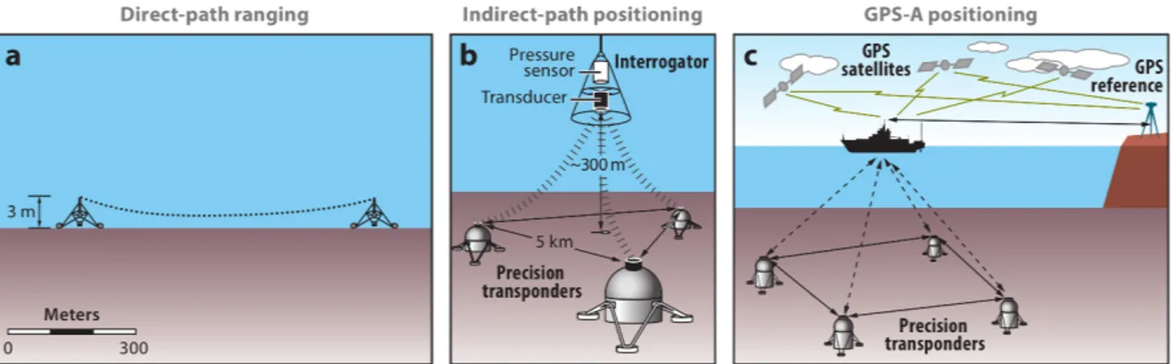
Figure 1.3.: Schematic diagrams of acoustic ranging methods to measure seafloor deformation (Bürgmann and Chadwell, 2014). (a) Direct Path ranging between two or more transponders to measure relative plate motion. (b) Indirect-path ranging of long distance transponders by an interrogator in between (c) GPS-A positioning by seafloor mounted transponders and buoy or ship GPS position to determine the absolute location in the global GPS reference frame.

Acoustic seafloor geodesy is distinguished in three different configurations: relative position measurements by direct-path ranging of two or more transponders, indirect-path positioning of long distance transponders and an interrogator in between to increase ranges, and GPS-

(11)

Chapter 1. Introduction 6 acoustic positioning (Figure 1.3).

The measurement of seafloor displacement by acoustic ranging between two fixed transponders or transponder to ship requires the transmission of precise sound signals. The time of flight can be measured with microsecond resolution, equivalent to mm of range (Bürgmann and Chadwell, 2014). Crucial to this approach is the determination of the sound wave propagation velocity on both end points or ideally along the acoustic path (Equation 1.1) by monitoring of temperature, pressure, conductivity or with high frequency sound velocity meters (Chadwell and Sweeney, 2010; McGuire and Collins, 2013).

v

sv

= 1 n

end⁄ start

v(x, y, z)ds (1.1)

Usually the two-way traveltimettwt is defined as time of flight from one transponder to another and the replying answer. The combined calculation of travel time and sound velocity results in the geometrical distance (Equation 1.2) between two transponders over a geological fault or plate boundary. Repeating interrogations over months and years yield the horizontal displacement.

s = v

sv

· t

twt

2 (1.2)

In 1996, Chadwick et al. (1999) deployed five direct-path ranging transponders across the active rift zone of Axial Seamount on the Juan de Fuca Ridge with a precision of≥1 cm over the distance of 100 m to 400 m. A previous deployment, in 1994, across the southern Juan de Fuca Ridge by Chadwell et al. (1999) revealed no significant measured extension. The acoustic ranging experiment by McGuire and Collins (2013) achieved a millimeter baseline

(12)

Chapter 1. Introduction 7 GPS-A combines GPS with acoustic ranging to measure the horizontal position of seafloor transponders with centimeter-level resolution in the same global reference frame as land- based GPS data. The lateral variation in sound speed is confined to the upper few hundred meters. Temporal variations have timescales from minutes to a couple of days caused by internal waves and currents and significantly affect the acoustic ranging resolution. These measurements are expensive and time consuming because the vessel must stay on station for several days to obtain a position with an accuracy of one centimeter. Moreover, intensive CTD measurements are required due to temporal and spatial sound speed changes.

In addition to the acoustic geodesy techniques, Absolute Pressure Gauges (APG) are a promising tool to measure vertical deformation on the seafloor. Atmospheric pressure sensors are commonly used in navigation applications to determine elevation. However, the relatively low density of atmospheric pressure confines the resolution to decimeters and limit the use as geodetic sensors. In the ocean, water is much denser and pressure increases with approximately 1 bar for every 10 meters in depth. Thus changes in depth are measurable by APG, which consist of a high precision quartz crystal resonator. Along with tilt meters to additionally measure the rotation along two horizontal axes, this approach yields a local measurement of the gradient in vertical deformation. Along the Hikurangi subduction zone in New Zealand, Wallace et al. (2016) investigated the fault slip behavior. A network of continuous APGs reveals the distribution of vertical deformation during a slow slip event.

They clearly demonstrated high precision pressure sensors as the appropriate instrument for vertical displacement.

1.4. Tectonic Setting

1.4.1. The North Anatolian Fault System

The North Anatolian Fault Zone is the most active fault zone in Europe as well as southwest Asia and de-couples the Anatolian Plate from the Eurasian Plate (McClusky et al., 2000).

The fault marks the northern boundary of the Anatolian Plate. The south-eastern boundary is characterized by the East Anatolian Fault, which extends from the Bingöl-Karlıova triple junction to the Cyprus Arc. Extensional forces of the Hellenic back-arc in the west and the collision of Arabia and Eurasia in the east result in a western motion and counterclockwise

(13)

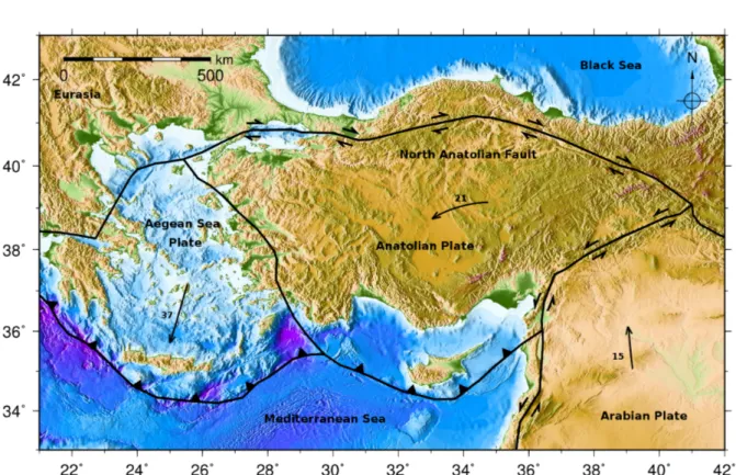
Figure 1.4.: The Anatolian Plate bounds in the north to the Eurasian Plate and in the south to Arabian and African Plates. Its westward motion and counterclockwise rotation result in the right-lateral North Anatolian Fault zone and the left-lateral East- Anatolian Fault (McClusky et al., 2000). Tectonic plate boundaries and motion vectors relative to Eurasia (from Bird (2003)). Global Multi-Resolution Topography (GMRT) from http://www.geomapapp.org (Ryan et al., 2009).

Figure 1.5.: The 20^th century earthquake sequence. Major events in Table 1.1. Rupture zones marked in different colors. Figure from Pinar et al. (2016).

The NAF is a 1200 km long right-lateral transform plate boundary between the Eurasian and Anatolian plates in northern Turkey (Figure 1.4). About 70 km east of Izmit the NAF splits

(14)

Chapter 1. Introduction 9 Year Latitude Longitude Mw Rupture Reference

[^¶N] [^¶E] [km]

2014 40.3 25.4 6.9 27 Bulut (2015)

1999 40.7 30.0 7.0 50 Ambraseys (2002)

1999 40.8 31.2 7.3 98 Ambraseys (2002)

1992 40.0 39.8 6.5 27 Bohnhoff et al. (2016) Stein et al. (1997) 1957 40.7 31.0 6.8 66 Ambraseys (2002) Stein et al. (1997) 1944 40.9 32.6 7.5 180 Stein et al. (1997)

1943 41.0 35.5 7.7 280 Ambraseys (2002)

1942 40.7 36.3 7.1 47 Ambraseys (2002)

1939 40.0 39.0 7.9 360 Ambraseys (2002) Stein et al. (1997)

1912 40.7 29.6 7.3 54 Ambraseys (2002)

Table 1.1.: Major historical earthquakes (Mw Ø 6.5) at the North Anatolian Fault (Fig- ure 1.5).

Its ends terminate at the back-arc extensional basin of the Hellenic subduction zone. The north-western section of the NAF is a very young strike slip fault zone, despite its beginning development in the east≥10 Ma ago ( engör et al., 2005). Focal mechanisms of earthquakes in the border region from the Anatolian Plate to the Aegean Sea Plate show east-west deformation and north-south extension (Jackson, 1994). The Euler pole of the counterclockwise rotation of Anatolia, respectively to Eurasia is located near the Sinai Peninsula at 30.7^¶ N, 32.6^¶ E 1.2^¶/Ma (Bird, 2003).

Consequently, the westward motion of the Anatolian plate results in strain accumulation along the transform faults zones of the NAF and Eastern Anatolian fault. Accumulated strain produces slip deficits and the probability of earthquakes. The cycle-like westward migration in the 20^th century earthquake sequence (Figure 1.5) started with the 1912 Mw 7.4 on the Ganos segment west of the Sea of Marmara and leaped to the eastern end with the 1939 Erzincan Mw 7.9 earthquake (Ambraseys, 2002; engör et al., 2005). Numerous earthquakes (Table 1.1) occurred subsequently along 720 km of the fault zone towards the west. In 1997, based on Coulomb failure stress calculation of the past 10 ruptures, Stein et al. (1997) proposed a 12 % probability for a large earthquake (Mw Ø 6.7) south of the western city of Izmit. Two years later on 17. August 1999 the 180 km long Izmit-Düzce segment ruptured in two events (Mw 7.4 and Mw 7.1) causing 17,000 casualties (Bulut, 2015). These events represent the termination of the current westward migration series.

Nonetheless, in 2014 the westward migration jumped to the North Aegean Sea (Mw 6.9) and

(15)

Chapter 1. Introduction 10 regime of the North Aegean Trough (Evangelidis, 2015). The not completed cycle along the North Anatolian Fault, precisely the remaining segments in the Sea of Marmara between the 1999 Izmit-Düzce segment and the 2014 earthquakes, are a seismic gap.

1.4.2. The Sea of Marmara

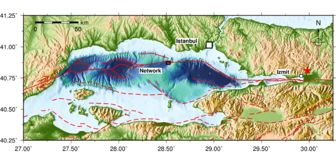
The Marmara Sea connects the Black Sea with the Mediterranean Sea and is roughly bounded by 40^¶N to 41^¶N and 26.5^¶E to 30^¶E. The Marmara Sea is a deep marine pull-apart basin with a shallow shelf in the south and consists of 3 sub basins in the north (Armijo et al., 2005). Tekirda basin, Central basin and Çınarcık basin are up to 1200 m deep and separated by bathymetric highs. The northern deep basins contain a significant load of sediments (1-2 km) (Le Pichon et al., 2001).

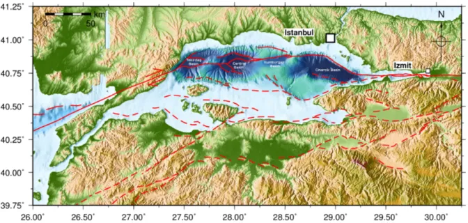
Figure 1.6.:Topographic map of the Marmara Sea. Red lines mark the main North Anatolian Fault by Armijo et al. (2005). Dash line mark the southern strand of the NAF. Bathymetric map of the Tekirda basin, Central basin and Çınarcık basin from Armijo et al. (2002). Global Multi-Resolution Topography (GMRT) from http://www.geomapapp.org (Ryan et al., 2009) In the Sea of Marmara the dextral strike-slip NAF opens into two major fault strands (Fig- ure 1.6), which are roughly 100 km apart before entering in the Aegean Sea. The Marmara

(16)

Chapter 1. Introduction 11 northward from the main branch to northern branches. Reflection seismic data and focal mechanisms of earthquakes show a series of pull-apart basins confined by a system of strike- slip and normal faults, which entail significant regional extension responsible for the formation of the Marmara Sea Basin (Ambraseys, 2002; Sorlien et al., 2012).

The focus of this thesis is the northern main strand of the NAF, which appears to concentrate most of the plate motion (McClusky et al., 2000). The active strike-slip faults that connect the Ganos fault with the Izmit fault are insufficiently understood as a result of the complex fault structure (Le Pichon et al., 2001). 2000 years of historical records prove the occurrence of large destructive earthquakes in the Sea of Marmara (Ambraseys, 2002) (Table 1.1). A total of nine M Ø 7 earthquakes occurred beneath or close to the Sea of Marmara with a repetition rate of ≥60 years (Parsons, 2004). The Main Marmara segment did not rupture since 1766 and in case of a locked fault the accumulated slip deficit is 5-6 m (Armijo et al., 2005; Hergert and Heidbach, 2010). Le Pichon et al. (2001) used short-term GPS models to derive slip partitioning in the Sea of Marmara and predict a right-lateral slip rate of 18- 20 mm/a and an extension rate of 8 mm/a across the northern Marmara Basins. In contrast, Ergintav et al. (2014) suggest that the Main Marmara Fault is aseismically creeping and the resulting slip-deficit is reduced to 2 mm/a. Based on GPS-geodetic stations on land the Marmara Sea is dominated by pull-apart tectonics and slip partitioning from enormous basins and small bends. The crustal scale of extensional strains and significant normal faulting presumably add complexity to the Marmara earthquake generation. However, geomechanical- models reveal a high strain accumulation rate of 10-16 mm/a at the Main Marmara Fault (Hergert and Heidbach, 2010; Armijo et al., 2005).

(17)

1.5. Objectives

The Kandilli Observatory and the Istanbul Technical University (Turkey) together with the University of Brest (France) and GEOMAR Helmholtz Centre for Ocean Research Kiel (Ger- many) initiated a joint project in the Marmara Sea to determine potential interseismic slip or strain accumulation on the North Anatolian Fault and its seismic potential. In addition, GEOMAR started to establish acoustical seafloor networks as an integral part of marine geodetic investigations. The Marmara Sea and tectonic condition of the NAF appear as the ideal opportunity to test geodetic underwater technology. Therefore, the following objectives guide the first GEOMAR geodetic deployment and will facilitate the evaluation of the technical and scientific achievements of this first application:

• The deployment and installation of a coherent working network of autonomous monitoring transponders across the North Anatolian Fault.

• Processing of the data and quality control of all measured parameters since only limited knowledge of previous deployments is available as the Sonardyne transponders were never installed in academia.

• The conversion from measured ranges to baselines between two or all stations in the network.

• Limitation in baseline measurement distance and occurring errors.

• Slip Estimation from the geometrical oblique distance measurements to potential right- lateral motion of the NAF to gain enhanced insight into the complex deformation pattern of strike-slip fault systems.

• The overachieving aim is twofold:

– Measuring baseline changes with the highest possible resolution.

– Resolving the deformation of the strike-slip fault, in particular to distinguish if the fault is locked or aseismically creeping.

(18)

CHAPTER 2 The GeoSEA-Project

In 2012, the GEOMAR Helmholtz Center for Ocean Research in Kiel established marine acoustic geodesy to monitor near real-time active seafloor displacement and strain in combination with passive seismicity recordings at active fault systems. The ProjectGeodesy at the Seafloor is BMBF funded and consists of 35 autonomous acoustic monitoring transponders by the manufacturer for acoustic positioning systems Sonardyne International Ltd. in the United Kingdom. The acoustic transponder systems have been deployed in three different target areas around the globe. All potential areas require previous high resolution mapping of the seafloor to determine the geological fault seafloor traces and to define the exact network configuration.

2.1. Methodology

The detection of seafloor displacements in millimeter precision over a reasonable time period with minimum errors in distance measurements is the primary objective of marine geodetic methods, requiring highly accurate measurements. In general, seafloor displacement occurs in vertical (z) and horizontal (x,y) directions. The vertical component is measured by pressure variations of the water column at the seafloor. Horizontal displacements can be measured in different ways (see chapter 1.3). The combination of repeated acoustic and GPS ranging provides absolute positions on the seafloor while long-term direct acoustic measurements between different transponders fixed on the seafloor provide continuous relative positions.

Here, the direct-path ranging method (Figure 1.3) to measure deformation on the seafloor

(19)

Chapter 2. The GeoSEA-Project 14 is applied.

Acoustic ranging methods provide relative positioning by using precision acoustic transponders. The Autonomous Monitoring Transponder (AMT) consist of high-precision pressure sensors, tilt meters and sound velocity sensors. The acoustic signals consists of an 8 ms phase-coded pulse with an 8 kHz bandwidth transmitted between transponders in a network to yield distances from two-way travel times and consequently deformation over time.

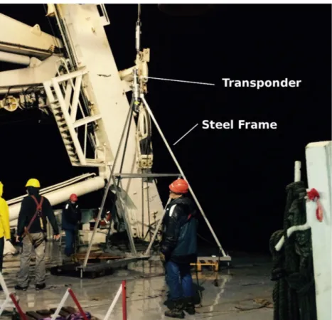
Figure 2.1.:Autonomous Monitoring Transponder mounted on GEOMAR tripod steel frame to measure horizontal displacement by acoustic ranging and vertical displacement by pressure sensors.

The Common Interrogation Signal (CIS) from one transponder transmitted to all other transponders in one network is a phase-encoded acoustic signal (Sonardyne, 2011). The eight milliseconds signal is converted to a low level alternating voltage at the acoustic transducer. Noise around the transducer is also converted into a electrical voltage noise and covers a wide frequency range. All the noise voltage and interrogating signals are amplified in the transponder pre-amplifier and the frequencies outside of the band used by the transponder channels are filtered. The transceiver unit uses a Digital Signal Processing algorithm by Sonardyne (2011) to identify the interrogation signal and to define the surrounding noise.

After the units individual time interval, named Turn Around Time (TAT), has passed, the transponder generates a powerful acoustic Individual Reply Signal (IRS). This reply is on a different channel than the interrogation signal. The transponder, which sends the interro-

(20)

Chapter 2. The GeoSEA-Project 15 The range or baseline between two AMTs can be now calculated with the equations (1.1) and (1.2):

s = (t

twt

≠ T AT ) · v

_sv

2 (2.1)

where ttwt is the two-way traveltime measured by the interrogating transponder and vsv is the average sound speed in seawater from both AMT velocity meter measurements.

Acoustic rays reflect at the seafloor, sea surface and interfaces in the water column. The reflected signal has increased in length, random phases and amplitudes. The transponder has a built-in blocking period to avoid any registration of reverberations or detection of other signals. The "blocking period" also prevents multiple replies from being transmitted in re- sponse to the reverberation of the initial interrogation signal. By using the equation (2.1) in combination with the function of sound velocity it can be illustrated that differences between the direct ray path and the bended ray path can be neglected.

(21)

CHAPTER 3 Geodetic Instruments and Data

The joint acoustic geodetic project in the Sea of Marmara started in October 2014. All ten acoustic transponders from the University of Brest and GEOMAR were successfully deployed by the research vessel "Pourquoi pas ?" on both sides of the Istanbul-Silivri-Segment (Figure 3.2). The four transponders belonging to the University of Brest are rated for 3000 m water depth and consist of glass spheres mounted on 3 m high tripods and an acoustic release for recovery. The GEOMAR transponders are mounted on 4 m high tripods made of stainless steel. The tripod height is necessary to ensure the acoustic visibility related to the direct wave propagation above the seafloor. Surface reflections and near-bottom refractions are inevitable but the AMT blocks all subsequent signals (Sonardyne, 2011). One transponder transmits phase-coded pulses with an 8 kHz bandwidth, the University of Brest (F-Stations) centered at 22.5 kHz and the GEOMAR (G-Stations) at 18.0 kHz, every two hours to all AMTs in the CIS network. The CIS interrogation ID range determine the network’s frequency bandwidth of the network and allows baseline measurements only in the same address range, thus a communication between the University of Brest and GEOMAR transponders is im- possible. CIS ID range of GEOMAR AMT stations is between the IDs 2301 and 2307 and for the Univ. of Brest AMT stations between the IDs 2001 and 2004. Hereinafter, all AMT transponders are indicated with station names (G1-G6) for the GeoSEA stations and not with the transponder specific CIS ID.

(22)

Chapter 3. Geodetic Instruments and Data 17

Figure 3.1.: Seafloor geodetic station on board of RV "Pourquoi pas ?" before deploying in October 2014. The transponder are mounted on top of the GEOMAR tripod steel construction.

The recorded data of travel times, sound speed, temperature, pressure and tilt are measured locally at the transponder and can be downloaded by an acoustic link with the high perfor- mance transceiver (HPT) even from small vessels. The HPT is connected to the Surface Interface Unit (SIU) on the vessel and can be controlled by Sonardyne Monitor software to check the transponder status and the downloaded data. The GEOMAR Monitor software downloads 9 Kb of data with 6000 bits/s before re-checking the acoustic link to the AMT on the bottom and preparing the next bytes.

The log period of the entire GEOMAR AMT network is two hours and starts with station G1 at 00:15 by sending the CIS signal to all AMTs and waiting for the reply signals. Mean- while, temperature, sound velocity and pressure are measured. Inclination, battery status and amount of data are less often recorded to save energy, as the sensors are not active every two hours. All AMT recording cycles are equally allocated in twenty minutes intervals to ensure constant time measurements of potential baseline changes as well as to ensure a

(23)

Figure 3.2.:The Sea of Marmara. Red lines indicate the North Anatolian Fault. The red star marks the location of the 1999 IzmitMw 7.6 earthquake. The high resolution bathymetry is shows the north Marmara Basins (the Tekirda basin, Central basin and Çınarcık), provided from Armijo et al. (2005). The geodetic network is located in the Kumburgaz basin (black rectangle).

sufficient time spacing between each AMT baseline measurement.

Since the deployment in October 2014, two service cruises with the RV Poseidon from GE- OMAR have been accomplished (Lange and Kopp (2015), Lange (2016)). In April 2015, the first data download yielded 6 months of data (Sakic et al., 2016). All AMT stations were active and downloading took 30 minutes for each ATM station. The second service cruise in April 2016, one year later, demonstrated that downloading of 430 kB of data reached the limit of viability. Downloading 700 pages in 6 to 18 pages intervals lasted for hours due to communication interruptions. In total, all stations recorded over 18 months continuous pressure, temperature, sound velocity, tilt as well as all potential baselines.

The data of station G5 could not fully be downloaded due to the limited cruise time on RV Poseidon. The data is missing from the beginning of March 2016 (Figure 3.3). The high-resolution temperature sensor of AMT G4 stopped measuring by an unknown sensor error in the end of December 2015. Note that the geodetic networks of University of Brest and GEOMAR are independent and not communicating among each other.

(24)

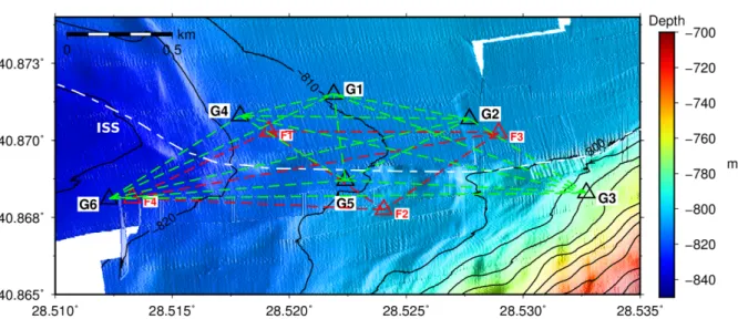
Figure 3.3.: The acoustic geodetic seafloor network in the Sea of Marmara. Bathymetry from high-resolution AUV mapping by Marmesonet (2009). The GEOMAR network: G1-G6, The Univ. of Brest network: F1-F4. green/red dashed lines indicate all potential Baselines in each network. The Istanbul-Silivri fault segment is marked as white dashed line traced from disrupted sediments in the AUV bathymetry. Transponder locations are based from the USBL positioning of the acoustic releaser during the deployment.

3.1. Energy Consumption

Before deploying the first acoustic geodetic network on the Marmara seafloor the energy consumption could only be estimated by analytic tests with the Sonardyne Monitor Software and manufacturer specifications. The retrieval date of the network was not finally set at the deployment in October 2014.

Each GEOMAR transponder contains 100 Ah of Lithium-ion batteries. These batteries have a flat voltage plateau which does not indicate the remaining energy in time but is expressed as percentage of the original capacity. Consequently, a contentious monitoring of the batteries is either done every 100^th measurement cycle, equally to 4.8 days. All AMT stations show a constant energy drain of ≥2.4 ± 0.1 %/month. The Sonardyne transponder will automatically switch to stand-by mode when 5 % of the energy is remaining to ensure the acoustic communication during recovery. Furthermore, to conserve energy the transponder goes into sleep mode, after all measurements are done. In addition, before the interrogation CIS signal is sent the transponder emitted a wake up signal to all transponders. After replying to the interrogation signal the AMT will return to sleep mode in a certain period of inactivity

(25)

Chapter 3. Geodetic Instruments and Data 20 (Sonardyne, 2011).

Station Battery Start Battery 04/2016 Battery Drain Stand-by Date

[ %] [ %] [%/month]

G1 99 59 2.4 03/2018

G2 100 61 2.3 05/2018

G3 100 60 2.4 04/2018

G4 99 56 2.4 02/2018

G5 100 63 2.4 05/2018

G6 100 58 2.4 03/2018

Table 3.1.: Energy consumption of the Marmara Sea GEOMAR transponder. All transponders show a similar energy drain.

The first transponder, namely G4, will approximately stop working in February 2018 and the other AMTs will follow step by step in stand-by mode (Table 3.1). The recovery of all geodetic transponders should be planned between February and May 2018 to guarantee GEOMAR’s first successful acoustic geodetic experiment in its entirety.

(26)

CHAPTER 4 Results and Discussion

In October 2014, the successful deployment and installation of an acoustic geodetic network was achieved and followed by two service cruises annually in April. The retrieved data consists of temperature, pressure, sound velocity, tilt and range measurements. These data are presented and discussed in this chapter. This thesis focuses only on data results of the GEOMAR AMT network as its first complete acoustic geodetic deployment. The Sonardyne

Figure 4.1.: The geodetic seafloor array in the Sea of Marmara. Bathymetry from high- resolution AUV mapping by Marmesonet (2009). The two way baselines are marked by green dashed lines. The one way baselines are marked by red dashed lines.

Monitor software exports all data of one AMT as a comma-separated CSV-file for further data processing. Each CSV-file consists of chronological records of all sensors and range measurements. The data processing was accomplished by Python moduleGEOSEA.py (Ap-

(27)

Chapter 4. Results and Discussion 22 language for multipurpose data processing. All functions were developed to create a tool for fast geodetic data processing. TheGEOSEA.py will be further developed to cope with new project demands and to solve upcoming problems. The first processing step is to sort all records according to their sensor and the delete error measurements with the intended function geosea.load_data() (Appendix B.1). The output consists of sorted files of each AMT transponder and also of each sensor separately. Recorded ranges revealed more baselines than initially expected. Besides the baselines from G6 to G2 and from G6 to G3, which are monitored in one way (Figure 4.1), all other baselines are continuously measured.

4.1. Temperature

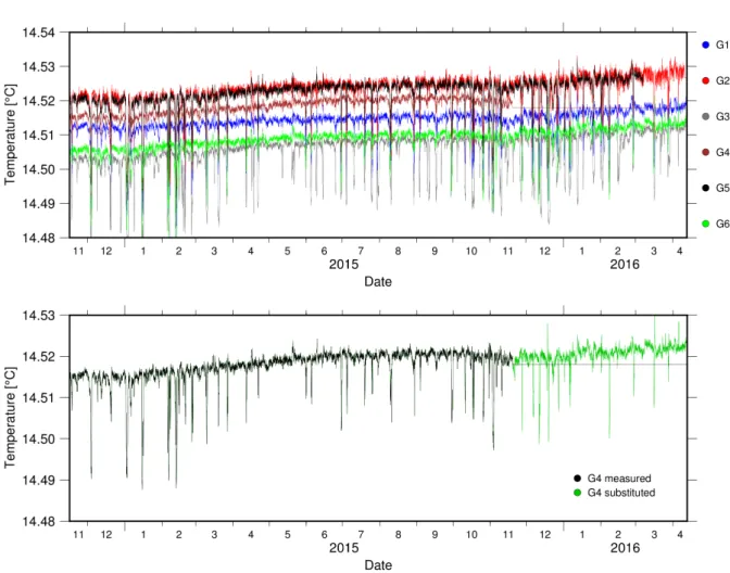
Figure 4.2.:High resolution temperature data measured from November 2014 to April 2016.

(28)

Chapter 4. Results and Discussion 23 HighResolutionTemperature sensors (HRT) measure the temperature in a two hour log pe- riod. Only AMT G4 stopped measuring in late December 2015 (Figure A.4). For further data processing the G4 HRT data is substituted from G6 with a constant shift of +0.00894 ^¶C.

AMT G6 is located close to G1 and shows an equal temperature trend. All HRT sensors show a continuous increase of 0.007^¶C/a and a total increase of 0.01 ^¶C after 18 month of recording. The temperature records show interruptions by cold water masses with a decrease of≥0.02^¶C in the otherwise homogeneous deep water close to the bottom of the Kumburgaz Basin. These cold water events occur every 6 to 20 days (Figure 4.2).

Excursus: Cold Water Events

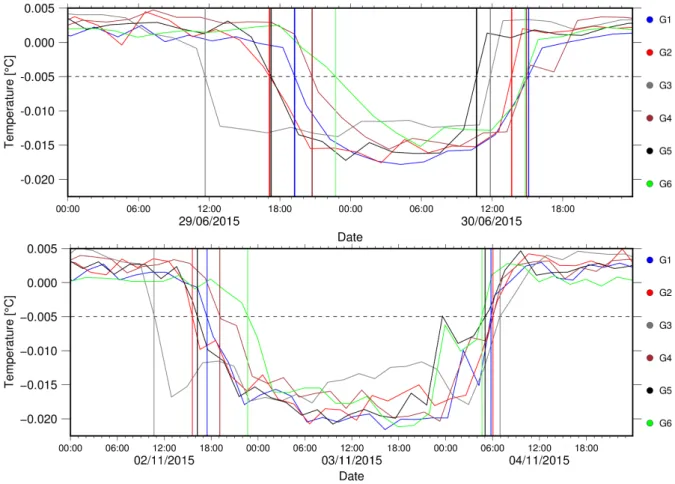
Figure 4.3.: The homogeneous deep water of the Kumburgaz Basin is interrupted by cold water events and shown are two events. The graphs show two events in June 2015 (top) and November 2015 (bottom). Note the fist AMT G3 recorded a temperature drop of 0.005^¶C and afterwards the stations G2 and G5 measured the temperature drop almost simultaneously six hours later. these results suggest an influx of water from east or south-east. The outflow

(29)

Chapter 4. Results and Discussion 24 The unexpected cold water events show a complex pattern and seasonal differences. Events in winter differ in strength and duration (Figure 4.2). The November 2015 cold water masses changed the ambient water temperature in the network for three days, until the AMT temperature sensors returned successively to previous temperature measured values (Figure 4.3).

In contrast, events during the summer show less decrease and duration, whereas direction retains all year. The temporal offset as shown in Figure 4.3 suggest a direction from south- east and approximate velocity of 0.1 km/h as AMT G3 recorded a decrease of 0.005 ^¶C at first and 5.5 h later almost simultaneously the AMTs G2 and G5. As a transition zone between two larger seas of opposing character, the Marmara Sea illustrates with presence of, relative to the predominant temperature, cold water masses in deep water. The cold water masses are an influence of the periodically circulation of low salinity jet flows from the Black Sea (Be iktepe et al., 1994). Timmermann (2016) analyzed the temperature data during her bachelor thesis and could not verify the origin of the cold water events by adopting the concepts of reverse hydraulic press and internal wave motion.

(30)

Chapter 4. Results and Discussion 25

4.2. Sound Velocity

The speed of sound in oceans is predominantly controlled by temperature, salinity and pressure. In shallow depth surface-driven mixing affects temperature and salinity, which influence mainly the sound velocity in water. Below 1000 m water depth temperature and salinity stabilize, the increasing pressure dominates the influence of sound speed.

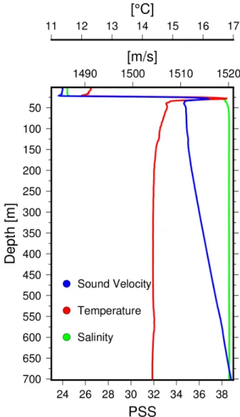
Figure 4.4.: Sound velocity profile 20 km southwest from the Marmara Sea network area (40.84^¶N 28.34^¶E). PSS is the Practical Salinity Scale from 1978 which is dimensionless.

The CTD data were recorded in December 1996 by SISMER (Systémes d’Informations Sci- entifiques pour la Mer) and are available by NOAA National Center for Environmental Infor- mation (Boyer et al., 2013).

(31)

Chapter 4. Results and Discussion 26 The upper layers in the Marmara Sea reflects mainly seasonal characteristics of Black Sea water heading through the Bosphorus as the result of the all-year sea level difference to the Aegean Sea (Be iktepe et al., 1994). Influenced by local heating/cooling and mixing, the halocline, the transition zone from low to high salinity water, varies between 25 m and 40 m. At 150 m water depth salinity and temperature stabilize and sound velocity is mainly controlled by pressure. The geodetic AMT stations are deployed in a depth of about 800 m, that means surface-driven mixing does not affect the baseline or sound speed measurements, as shown in Figure 4.4.

The GEOMAR transponders measure sound velocity by the Valeport Ltd. "Time of Flight"

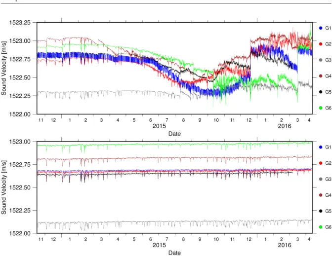
sound speed sensor of 10 mm length. Following the first data recovery, it became already apparent that the cold water events generate devastating spikes in the sound velocity measurements, which again triggered increasing sensor drift (Figure 4.5). These artifacts of the sound velocity sensor result in centimeter artifacts in the converted baselines. The only way to handle the long-term instability of the sound speed sensor is the estimation of sound speed using temperature, pressure and salinity. Salinity is not measured by the AMT’s and a constant salinity of 38.6 practical salinity unit (PSU) in 800 m depth is assumed, which is derived from the measured CTD (Figure 4.4).

Empirical sound speed formulas (Wilson, 1960; Del Grosso, 1974; Leroy et al., 2008; Chen and Millero, 1977), computed from in-situ measurements of seawater temperature, pressure and conductivity using a laboratory-determined relationship, provide equal sound velocity resolution but differ in scale. Leroy et al. (2008) proposed a sound speed equation in seawater is a function of temperature, salinity, depth, and latitude in all oceans and moreover in equal scale to AMT measurements. The Python Module ’Geosea.py’ implements the sound speed calculation functions of Leroy et al. (2008); Wilson (1960); Del Grosso (1974) (Appendix B.2). Figure 4.5 shows the comparison of AMT measured and calculated sound velocity and elucidated the cold water initiated sensor drift. All calculated velocities increase slightly due to increasing temperature.

(32)

Figure 4.5.: (Top) Sound speed data measured by Valeport velocity meters. Note the short-term and long-term drift up to 0.5 m/s resulting from cold water events. (Bottom) Recalculated sound speed by using Leroy et al. (2008) formula with measured pressure and temperature data and constant salinity of 38.6 PSU.

4.3. Pressure

The AMT pressure data show higher amplitude variations in winter months compared to the summer seasons. The seasonal variations differ from approximately ±50 dbar to ±10 dbar (Figure 4.6). In general, the Sea of Marmara is a region of low tidal amplitudes and long- period oscillations (Yüce, 1993). Long period oscillations exist due to the long-period tidal constituents and meteorological influences. The mean water level is inversely related to the barometric pressure. It is evident from the Marmara Sea AMT observations that the long-period seasonal oscillations are meteorological induced. The distance to the Bosphorus Strait and Dardanelles results in isolation from the semi-diurnal tidal oscillations of Aegean and Black Sea. Tidal constituents can be analyzed with the recorded pressure data by the Python Module Pytides.py. The prevalent tidal constituents are S6 and OO1, both are di-

(33)

Chapter 4. Results and Discussion 28 urnal and superimpose less dominant semi-diurnal variations.

Figure 4.6.: Pressure data of AMT G1 with a sampling rate of 2 hours. Meteorological oscillations and long-period tidal constituents are clearly visible. All AMT pressure data are presented in Appendix A.2.

The pressure data are important to recalculate the sound velocity (Leroy et al., 2008), additionally, the pressure sensors can also be used as APG to derive vertical motion. Vertical displacement may occur on a strike-slip fault through partitioning of fault motion and generation of pop-up structures or pull-apart basins (Figure 1.1). The AUV bathymetry in Figure 4.1 shows indications for slightly vertical deformation along the NAF, but all AMT stations except G5 are not located on top of the disrupted sediments. However, within the raw data no vertical movement can be resolved and is therefore suggested to be smaller than 0.1 cm. The measurement of vertical displacement requires further steps in the removal of tidal oscillations.

4.4. Tilt

Inclination measurements in terms of tilt motion are recorded at each AMT. For the baseline length the stability of the tripod on the seafloor is crucial. All stations settled in the first two weeks after deployment. AMT G3 was deployed with a total inclination of 10.5°(Figure A.15).

Pitch and roll are indistinguishable due to the unknown orientation of each transponder,

(34)

Chapter 4. Results and Discussion 29 though two orthogonal components provide the true amount of tilt without orientation. The total tilt can be calculated with:

Tilt

max

=

^Ò

Pitch

²

+ Roll

²

(4.1)

Figure 4.7.: Pitch and roll of station G4. At the end of September the station shows a slight change in the roll component, which is too small to affect the baselines. All inclination plots are presented in Appendix A.3.

Station G4 shows a change of -0.115° in the roll component at the end of September, but the total inclination change is insignificant with -0.006°. All other AMT stations are stable in time, but with different pitch and roll (Appendix A.3). The conversion of tilt motion to range variation for specific baselines is not feasible due to the unknown tilt orientation. Maximum baseline change for a tilt of 0.005° would result in 2 cm baseline change by assuming a tripod height of 4 m. Furthermore, the GEOMAR tripod constructions (Figure 2.1) are less tilting on the seafloor as the transponders of University of Brest with their buoyancy of glass spheres (Sakic et al., 2016).

(35)

4.5. Baselines

The acoustic baseline data processing consists of a conversion from time of flight between two AMT transponders to length by using equation (2.1) implemented inGeosea.py-Python Mod- ule (Appendix B.3). The sound speed along the ray path can be approximated by equation (1.1) with sound speed average from both AMTs. The converted time of flight measurements generate an individual scatter of distances due to temporal sound speed changes and sound speed uncertainty along the ray path (Figure 4.8). Additionally, cold water events affect sound speed and baselines and can be identified as such as temporary deflections in the time series. A moving average of fourteen days smoothes the baseline scatter and illustrates relative baseline changes in time.

The Marmara Sea geodetic network measures fifteen baselines in total (Table 4.1) consisting of nine crossing the North Anatolian Fault and six either north or south of the fault (Fig- ure 4.1). The baselines are suffered by constant salinity uncertainty in Leroy et al. (2008) sound speed formula and ray path, therefore, baselines include water column heterogeneity and seafloor deformation. Figure 4.9 demonstrates the relative baseline changes as a conse- quence of changes in temperature and salinity. Long-term changes in salinity are unknown and would influence the length of all baselines in a similar way.

An increase of temperature of 0.007 ^¶C/a can be observed and would result in a length change of 1 cm for a 500 m long baseline. As shown above, all stations show an temperature increase which would indicate one constant sensor drift for all stations. Significant sensor drift is unlikely since length changes are generally less 1 cm/a. Such a coherent long term signal is not observed and presumably would show a seasonal effect. If the 0.007 ^¶C/a are caused by sensor drift, all baselines should show a continuous increase of baseline length.

Nevertheless, the data showed no evidence of a common increase of Ø1 cm/a.

(36)

Figure 4.8.:Baselines of AMTs: G1-G2 (Top) and G4-G6 (Bottom). The respective moving average of fourteen days is shown as a solid line. All ranges from and to AMT G4 consisting of a higher sound speed uncertainty due to under laying temperature for baseline for G4 is taken from AMT G6 after December 2015.

4.5.1. Baseline Resolution

Sound speed uncertainty ultimately limits network sizes to a few kilometers before acoustic- derived distance uncertainty exceeds anticipated deformation signals (Chadwell and Sweeney, 2010). The fifteen measured baselines (Appendix A.4) show continuously tubular scatters over time with varying width. Therefore, analysis of baseline uncertainty yields the assumable resolution. The standard deviation quantifies the amount of variation and dispersion in a time series around a mean. Equation (4.2) defines the standard deviation, whereX_i are the baseline measures and X is the overall average. The result shows an empirical correlation coefficient of 0.9 (Figure 4.10) implying that the standard deviation of baselines raises linearly

(37)

Figure 4.9.:Baseline changes caused by changes in salinity and temperature. An increase of 1 cm in baseline length results in an increase of 0.0062°C or 0.0159 PSU. Note the relation between temperature, salinity and sound speed is not linear, however, the intervals considered here are small and the dependencies of temperature and salinity for the given x-axis spatially coincide.

with an increase of baseline length.

SD =

ˆı ıÙ

1 1 ≠ n

ÿn

i=1

(X

i

≠ X )

²

(4.2)

Three baselines with lengths over 1000 m are measured, G3 and G4 to G6 are the longest ranges with 1329.9 m and 1717.8 m, respectively. These baselines exceed the standard deviation of 0.7 cm (Table 4.1). The third baseline from G3 to G4 is 1278.1 m long and shows standard deviation of 0.6 cm. The linear regression suggests that ranges over 2300 m can pass the standard deviation of 1 cm. These results from the Marmara Sea network demonstrate that baselines up to 1000 m length do not exceed the resolution of 5 mm. Consequently, if the standard deviation increases linearly with baseline length, than distances over 2000 m can be measured in complex widespread deformation areas without loss in strain resolution.

(38)

Figure 4.10.: Standard deviation in centimeter of converted baseline scatters. Note all standard deviations (SD) show a linear increase, with an empirical correlation coefficient of 0.9, related to its length. AMT distances less 1000 m reveal, in most cases, a standard deviation below 5 mm (dashed line).

4.5.2. Theoretical Ray Approach

The maximum resolution is limited by the sound speed heterogeneities along the ray path and increases with distance (Chadwell and Sweeney, 2010). To show the maximum resolution of baselines theoretical travel times are estimated. The synthetic ray approach by Slotnick (1959); Slawinski and Slawinski (1999) considers a Vertical-Seismic-Profile (VSP) source- receiver geometry used for seismic measurements in boreholes. Here, I consider one way travel time as the CIS signal from one AMT to another transponder. Ray trajectory in medium of constant increasing sound speed v(z) = a+bz is determined from Fermat’s principle ”^s ^ds_v = 0 and Snell’s Law with the constant ray parameterp© ^sin◊_v (Figure 4.11).

Integratingv(z) and yield the expression forX and solve the equation forpSlotnick (1959) with X as offset and depth Z:

p = 2bX

ÚË

(bX )

²

+ v

₁²

+ v

₂²^È

≠ [2v

1

v

₂

]

²

(4.3)

with limxæ0p= 0 and limxæŒp= 0 the ray reaches the transponder vertically, however in direct path ranging only short offsets exist.

(39)

Figure 4.11.: Direct acoustic geodesy geometry as deployed in the Sea of Marmara. One AMT acts as source and another as receiver. The lateral distance between both AMT is defined as x and the vertical depth as z. The ray path element is ds = (dx, dz) = (ds sin(◊), cos(◊))where◊ describes the angle in between (Slawinski and Slawinski, 1999).

The AMT transponder is mounted on top of the GEOMAR tripod construction.

The time of flight for the direct arrival is t =^s _v(z)^ds =^s₀^z ^dz

vÔ

1≠p²v² and by integrating with ray parameter p in equation (4.3) and sound velocity we obtain (Slotnick, 1959):

t = 1 b ln

S U

Q

a

1 ≠

^Ò

1 ≠ (pv

1

)

²

1 ≠

^Ò

1 ≠ (pv

2

)

²

R b T

V

(4.4)

wherev1is the measured sound speed at the source AMT andv2 the sound speed measured at the receiver AMT. For each sound speed measure at both endpoints the theoretical traveltime is calculated by assuming no deformation as a constant offset between the station inxandz.

All sound velocity effects such as cold water events or seasonal tides generate remarkable spikes in theoretical baseline time series (Figure 4.12). The obtained scatter deviation is 1.33 mm or 65 % narrower as the converted time of flight by neglecting the cold water outcrops. Note that most cold water events are not affecting the measured baseline. In real data the cold events are not always seen in the baselines. In this case, the velocity changes from the cold water events are compensated by the travel time.

(40)

Chapter 4. Results and Discussion 35 are not measured instantaneously. Temperature and pressure are only measured during the interrogating call of the AMT every 120 minutes. The replying AMT does not measure temperature and pressure at the same time with the interrogation AMT, but when sending its interrogation signal CIS. As a result pressure and temperature from both stations are shifted up to half a log period of 60 minutes. Therefore, the synthetic baselines, which are based on measured temperature and pressure from two AMTs, include the effect of changes in the water column and spatial heterogeneities. Sound speed estimates are once in the logging period of two hours in contrast to range measurements, which are recorded every twenty minutes.

Figure 4.12.:(Top) The converted baseline calculated sound speed (Leroy et al., 2008) with the moving average of fourteen days as solid line. (Bottom) The same baseline calculated by theoretical traveltime (Equation 4.4) and a constant sound speed of 1520 m/s. Both baselines are based on the same temperature and pressure data and only differ in travel time.

The baseline change seen with the measured can only result because of salinity changes or true deformation of the seafloor.

(41)

4.6. Relative Slip Rate Estimation

Six months of monitoring was too short to model fault motion and slip evidence could not be observed (Sakic et al., 2016). Here, eighteen months of data provide the first direct measured slip rate assumption. The resulting baseline changes derived from moving averages reveal complex pattern of apparent lengthening/shortening. GPS-land investigations indicate significant deformation as aseismic creeping can be detected, in contrast, based on the offshore geodetic results, no evidence for right-lateral strike slip motion is observed. Constant creep primarily due to slip partitioning and internal deformation modeled for the three-dimensional Main Marmara Fault system segment suggests complex subsurface sediment deformation (Hergert and Heidbach, 2010; Reilinger et al., 2006). The fault trace is visible in the geodetic network area as a vertical sediment disturbance in high-resolution AUV bathymetry and indicates a narrow deformation zone, however less active fault traces are found north and south of the study area and suggest a widespread deformation zone of about 1 km with the highest slip rates at the main fault segment and much lower slip rates at secondary faults (Le Pichon et al., 2001).

Figure 4.13.: Results of 1.5 years of monitoring the Main Marmara strand obtained close to zero slip rates. No evidence of right-lateral deformation is observed. The highest slip rate occured on the western baseline G4-G6 and can be related to extensional forces of the detected normal fault scarp splitting of the fault (Grall, 2013). The North Anatolian fault is marked by white dashed line and the expected normal fault by thinner white dashed line.

The region of potential extension is marked by a question mark.

(42)

Chapter 4. Results and Discussion 37 The maximum range length between two AMTs is limited due to the uncertainties of sound speed along ray path and increases linearly with distance (see Figure 4.10) (Bürgmann and Chadwell, 2014; Chadwell and Sweeney, 2010). This relation was previously found for other offshore geodetic networks. Consequently, the southern AMT stations are located very close to the fault trace to ensure a small uncertainty and best resolution. Most baselines north, south and crossing the NAF become longer with rates close to zero and show small shortening perpendicular to the fault (Figure 4.13), however, these baseline changes exclude any seafloor deformation larger than a few mm/a (see Section 4.5.1) (Table 4.1). The baseline lengthening/shortening rates and orientation by Sakic et al. (2016) based on least square inversion are inline with results obtained here by considering constrained sensor drifts, despite the overestimated deformation rates. The highest baseline change rate of 0.7 cm/a between the AMTs G4 and G6 (Appendix A.32), located in the western part of the network, is less than the modeled deformation rate of ≥1.2 cm/a of Sakic et al. (2016). A normal fault scarp detected 150 m west of AMT G4 (Grall, 2013; Armijo et al., 2005) could ex- plain the lengthening of the baseline G4-G6 (Figure 4.13). The baseline samples only the southern termination of this fault. Taking into account that only this baseline crosses the extensional domain is not conclusive. The normal fault scarp can also represent a possible pull-apart structure related to a releasing bend (see Figure 1.1) developing in the northern Kumburgaz basin alongside the Central Marmara Ridge. Slip partitioning at a step over can reduce the predicted slip rate to the half of the dextral strike-slip motion. Active releasing bends generate subsidence due to the extensional forces. This vertical displacement can potentially be observed over time by pressure sensors. This requires subtraction of the tide signals and complex data processing, which is beyond the scope of this thesis. Pull-apart structures cutting the Main Marmara Fault are relevant to discuss elsewhere for a potential single rupture or several smaller events along the Marmara seismic gap (Le Pichon et al., 2003; engör et al., 2005; Sorlien et al., 2012).

The baseline change rates did not show any evidence of creep at least less than 5 mm/a considering the measurement resolution from standard deviation. This deformation is clear less than the predicted slip rates of the North Anatolian Fault (Reilinger et al., 2006; Hergert and Heidbach, 2010). As result of the nearly zero slip rates/deformation, the Marmara fault zone is continuously accumulating strain. Assuming the limit of 5 mm/a as slip resolution (Section 4.5.1) comparing it with the estimated slip of 16 mm/a by Hergert and Heidbach (2010); Hergert et al. (2011) results in a strain accumulation of more than 11 mm/a. This corresponds with the direct observation of strain accumulation of 10-15 mm/a at the Princes

(43)

Chapter 4. Results and Discussion 38 No. Baseline Length X [m] Change Rate [cm/a] Relative Change [cm] Figure

1 G1 - G2 500.046 0.183 0.275 ±0.32 A.19

2 G1 - G3 977.209 0.102 0.153 ±0.54 A.20

3 G1 - G4 345.413 0.271 0.406 ±0.30 A.21

4 G1 - G5 363.635 -0.149 -0.224 ±0.23 A.22

5 G1 - G6 887.267 0.438 0.725 ±0.31 A.23

6 G2 - G3 497.148 0.192 0.288 ±0.26 A.24

7 G2 - G4 829.408 -0.086 -0.043 ±0.48 A.25

8 G2 - G5 515.135 -0.111 -0.166 ±0.35 A.26

9 G2 - G6 1329.898 0.288 0.432 ±0.72 A.27

10 G3 - G4 1278.139 0.310 0.465 ±0.64 A.28

11 G3 - G5 854.976 0.182 0.273 ±0.39 A.29

12 G3 - G6 1717.838 0.375 0.563 ±0.74 A.30

13 G4 - G5 484.287 0.216 0.324 ±0.27 A.31

14 G4 - G6 553.923 0.703 1.055 ±0.38 A.32

15 G5 - G7 863.067 0.367 0.551 ±0.28 A.33

Table 4.1.: Baseline change rates obtained from moving average of fourteen days method of range and sound speed conversion. Standard deviation is attained from baseline scatter and is correlating with the baseline length. Note the deformation rate does not exceed the standard deviation except of the two baseline G6-G1 and G6-G4.

Island Segment (Ergintav et al., 2014).

Since the last rupture of the Marmara Segment in 1766, a constant slip of 11 mm/a results in a slip deficit of 2.75 m along the fault. Consequently and in accordance with other seismic assessments (Hubert-Ferrari et al., 2000; Le Pichon et al., 2001; Ergintav et al., 2014; Bohn- hoff et al., 2016; Murru et al., 2016), the 70 km long Istanbul-Silivri-Segment is capable of an earthquake Mw>6 and poses an enormous seismic hazard for Istanbul and other cities around the Sea of Marmara.

(44)

CHAPTER 5 Conclusion

The time series of the seafloor geodetic network installed in the Marmara sea provides results of the complex deformation of the North Anatolian Fault system. The Autonomous Monitor- ing Transponder system is the first to be used to observe seafloor deformation directly as a scientific problem. Software and hardware are easy to use as well as learn and once deployed individual configuration data download and communication are possible. The Marmara Sea network as a technical test for further geodetic projects turned out to be very successful.

In total, fifteen acoustic ranges across and on the same side of the fault are measured over 1.5 years with a logging period of two hours yielding more than 6500 records of each baseline pairs. Horizontal ranges from 363 m up to 1717 m are reached with a resolution from 3 mm to 7 mm. Direct-path acoustic ranging provides baselines in millimeter precision of seafloor displacement across geological faults or ridges over more than 1000 m distances. Baseline resolution is shown to be linearly related to distance. Hence, future deployments need to consider the maximum range length with respect to expected deformation rate. For example, aseismically creeping faults require a narrowly positioned network to resolve the same strain as long distance measurements at fast slipping transform faults like the East Pacific Rise (McGuire, 2008). Subsea deployment sites in target areas have to be selected with the compromise between too deep seabed such as trench zones and deep enough for insignificant seasonal water mass influences.

Data conversion and modeling indicates that surface deformation does not exceed the reso-

Strain measurement across the North Anatolian Fault in the Sea of Marmara

Acoustic Seafloor Geodesy: