in the Central North Sea:

(1)

Contents lists available atScienceDirect

International Journal of Greenhouse Gas Control

journal homepage:www.elsevier.com/locate/ijggc

Footprint and detectability of a well leaking CO

2

in the Central North Sea:

Implications from a field experiment and numerical modelling

Lisa Vielstädte

^a,^⁎

, Peter Linke

^a

, Mark Schmidt

^a

, Stefan Sommer

^a

, Matthias Haeckel

^a

, Malte Braack

^b

, Klaus Wallmann

^a,^⁎

aGEOMAR Helmholtz Centre for Ocean Research Kiel, Germany

bDepartment of Applied Mathematics, University of Kiel, Germany

A R T I C L E I N F O Keywords:

Carbon dioxide Geological storage Leakage North Sea Sleipner Wells

A B S T R A C T

Existing wells pose a risk for the loss of carbon dioxide (CO2) from storage sites, which might compromise the suitability of carbon dioxide removal (CDR) and carbon capture and storage (CCS) technologies as climate change mitigation options. Here, we show results of a controlled CO2release experiment at the Sleipner CO2

storage site and numerical simulations that evaluate the detectability and environmental consequences of a well leaking CO2into the Central North Sea (CNS). Our field measurements and numerical results demonstrate that the detectability and impact of a leakage of < 55 t yr⁻¹of CO2would be limited to bottom waters and a small area around the leak, due to rapid CO2bubble dissolution in seawater within the lower 2 m of the water column and quick dispersion of the dissolved CO2plume by strong tidal currents. As such, the consequences of a single well leaking CO2are found to be insignificant in terms of storage performance. Only prolonged leakage along numerous wells might compromise long-term CO2storage and may adversely affect the local marine ecosystem.

Since many abandoned wells leak natural gas into the marine environment, hydrocarbon provinces with a high density of wells may not always be the most suitable areas for CO2storage.

1. Introduction

Geological storage of carbon dioxide (CO2) aims at reducing the amount of anthropogenic CO2added to the atmosphere (e.g.Metz et al., 2005) and plays a role in various carbon dioxide removal techniques that have been proposed to reduce the CO2content of the atmosphere (IPCC, 2014). In Europe, the largest potential to store CO2is offshore (∼240 Gt of CO2) mostly in deep saline aquifers (e.g.EU GeoCapacity, 2009). More than 80% of the European offshore storage capacity is located in Norwegian waters (EU GeoCapacity, 2009), where Statoil operates the world’s first large-scale CO2storage project “Sleipner” with an annual injection rate of ∼1 Mt of CO₂since 1996 (Fig. 1). Here, CO₂ from natural gas production is injected into a saline aquifer in ∼900 m sediment depth, overlying the geological gas reservoir where it is ex- tracted from (Torp and Gale, 2004;Arts et al., 2008). As such, Sleipner and many other large-scale CO2storage projects are located in regions that have already been exploited for hydrocarbon production. This has several benefits as compared to undeveloped sites: 1) they tend to be geologically well-understood with existing wellbore and seismic data helping to characterize the local geology and overburden, and 2) may

already have infrastructure in place (Jordan et al., 2015). One down- side of storing CO₂ in developed sites is the presence of pre-existing wells (Gasda et al., 2004;Nordbotten et al., 2005), which have been identified for posing a greater risk for gas leakage from CO2storage formations than natural geological features, such as faults or fractures (Bachu and Watson, 2009). However, so far, there is no evidence for CO2 leakage through wells, faults, and the overburden at Sleipner (Eiken et al., 2011;Chadwick et al., 2009) indicating that CO2is safely contained within the storage complex.

Concern about CO2leakage along abandoned wells is widely at- tributed to well barrier failures (Gasda et al., 2004;Nordbotten et al., 2005;OSPAR Convention, 2007;EU CCS Directive GD1, 2011), where CO2may escape from the storage reservoir either due to pre-existing failures in the well material or due to subsequent corrosion of the cement and steel casings that are exposed to the subsurface CO₂plume (Kutchko et al., 2007;Carey et al., 2010,2007;Crow et al., 2010), but were originally not designed to withstand CO2 (Bachu and Watson, 2009). Estimates on CO2gas flows associated to this kind of leakage are low: 0.1 kg yr⁻¹for leakage along a well with degraded cement (Jordan et al., 2015), less than 0.1 t yr^-1for leakage along a well with sustained

https://doi.org/10.1016/j.ijggc.2019.03.012

Received 10 July 2018; Received in revised form 5 March 2019; Accepted 13 March 2019

⁎Corresponding authors at: GEOMAR Helmholtz Centre for Ocean Research Kiel, Wischhofstr. 1-3, D-24148 Kiel, Germany.

E-mail addresses:lvielstaedte@geomar.de(L. Vielstädte),kwallmann@geomar.de(K. Wallmann).

International Journal of Greenhouse Gas Control 84 (2019) 190–203

T

(2)

casing pressure (Tao and Bryant, 2014), and 0.3–3 t yr^-1 for poorly cemented wells (Jordan et al., 2015) with a typical wellbore cement permeability below 1 Darcy (Crow et al., 2010). Higher leakage rates, on the order of 3–52 t yr^-1of CO2(Vielstädte et al., 2015,2017; Bachu, 2017), may arise from gas losses along the outside of wells, where drilling has disturbed and fractured the sediment around the wellbore mechanically thereby creating highly efficient pathways for the upward migration of gas (Gurevich et al., 1993). This kind of leakage has re- cently been observed at abandoned gas wells in the CNS, where bio- genic methane, originating from a shallow (< 1000 mbsf) gas source in the sedimentary overburden above the deep hydrocarbon reservoirs, leaks into seawater (Vielstädte et al., 2015; 2017). Shallow gas leakage is presently not targeted by regulatory frameworks except in Alberta (Canada), but may have important implications for CO₂storage in developed hydrocarbon provinces with high well density especially in shallow strata above deeper hydrocarbon reservoirs.

Here, we focus on the Sleipner CO2storage site(Fig. 1A) and in- vestigate hypothetic, but realistic leakage of CO2 along a well that penetrates the subsurface CO2plume and leaks into the ∼80 m deep water column, using a combination of experimental field data and numerical modelling. The main objectives of this study are to predict the spatial footprint, detectability, and environmental consequences of a well leaking CO2at realistic rates and under real tidal forcing by ana- lyzing an existing bubble dissolution model and a newly developed plume dispersion model against the data collected from anin situCO2

leakage experiment. Results presented in this study are directly ap- plicable to most global offshore CO₂storage sites, which are planned for hydrocarbon provinces, where ubiquitous hydrocarbon infrastructures pose a risk for the upward migration of gas. This study further fills a gap in CO2storage-related field experiments and hydrodynamic modelling research, which mostly operated at large scales and high rates addres- sing the release of CO2 during a highly unlikely blowout scenario (Phelps et al., 2014; Dewar et al., 2013; Hvidevold et al., 2015;

Greenwood et al., 2015;Dissanayake et al., 2012) and leaky fault scenario (Kano et al., 2010) or have investigated leakage at low rates into shallow coastal waters (i.e. QICS experiment; Blackford et al., 2014;

Dewar et al., 2015; Mori et al., 2015;Sellami et al., 2015), with hydrodynamic properties that are not representative for submarine

storage projects that are operating or are under consideration in the open North Sea.

2. Materials and methods

During the Celtic Explorer expedition CE12010 (July-August 2012), a controlled gas release experiment (GRE) was conducted at 81.8 m water depth to simulate leakage of CO₂ into the North Sea water column in the vicinity of the Sleipner CO2storage site (Fig. 1, section 2.1). A gas bubble dissolution model (BDM;Vielstädte et al., 2015) was applied to calculate the rate of CO₂ dissolution in seawater (section 2.2). The resulting rate was used as input parameter for the plume dispersion model (PDM) that was applied to simulate the spread of dissolved CO2in the water column (section 2.3). Both models were calibrated against the observational GRE data (section 2.4). Subse- quently, the calibrated models were applied to compute three leaky well scenarios covering the range of possible emission rates (section 2.5).

2.1. Gas release experiment (GRE)

Three pressure bottles of CO2(50 L, 57 bar), one smaller bottle of Krypton (10 L, 250 bar), which was used as a tracer gas, two battery packs, a gas control unit, and release head, were mounted to the Lander system (“Ocean Elevator”, Linke et al., 2015) and deployed video- guided at the seafloor (58°24′22.41″N, 2°1′25.54″E,Fig. 2). The control unit included a spiral coil and a heated pressure regulator to reduce the pressure of the outflowing gas from up to 250 bar inside the gas bottle to 11 bar before the gas entered the microcontroller, which regulated the gas flow (Fig. 2C). Bubbles were generated on top of the Ocean Elevator by seven 1/8” stainless steel tubes connected by valves and covered by plastic heads which were pierced by three 8 mm holes each (Fig. 2B). At a preset gas flow of 30 L min⁻¹at STP (25 °C, 1 bar), a total of 40 kg of CO2was released into the water column over a period of 11.5 h. This corresponds to an annual leakage rate of 31 t yr⁻¹of CO2, which falls in the upper range of methane gas fluxes observed at abandoned wells in the CNS (Vielstädte et al., 2015).

The gas discharge was observed in situ during a 4 h dive with the Fig. 1.A) Overview map showing the location of the study area (red star) in the CNS. B) Map of the study area showing the Sleipner CO2

injection point (yellow star), the pre- dominantly north-eastward extension of the CO2plume within the ∼900 m deep Utsira sand formation (colored contours), the location of the gas release experiment (GRE, black flag, 58°24′22.41″N, 2°1′25.54″E), and the location of wells (circles) in the area. Platform wells (orange circle) from which the CO2is injected and those which have been identified to leak shallow gas (wells 15/9-13 and 16/7-2, Vielstädte et al., 2015) are highlighted.

(3)

remotely operated vehicle ROV Kiel 6000 (GEOMAR Helmholtz- Zentrum für Ozeanforschung Kiel, 2017) equipped with HD camera/

video device and a sonar system. The sonar system was used to navigate the ROV downstream of the artificial CO2leak by tracking the less so- luble and ∼27 m high Krypton gas flare. The spread of the dissolved CO2plume was monitored geochemically using the commercial HydroC pCO2 sensor (S/N 0412-006, Kongsberg Maritime Contros GmbH) mounted to the front porch of the ROV. The sensor was calibrated for pCO2signals up to 3000 μatm (accuracy ∼1% of reading resolution;

resolution: < 30 μatm as described by Fietzek et al., 2014) and was programmed to measure in 60 s intervals, which is equal to the sensor’s response time (Fiedler et al., 2013). For a better navigation of the ROV in the plume, HydroC sensor data were, in addition to internal data recording, transferred as an analog voltage signal which enabled online reading of the pCO2signal during ROV operation. ROV-operated pCO2

surveying was performed in different vertical heights and distances downstream of the artificial leak, remaining at each measuring position for at least 10 min to obtain a representative pCO2signal. At the end of the experiment a vast number of hagfish visited the release site, potentially attracted by the smell of dead meio- and macrofauna in the sediment. Unfortunately, ship time was too limited to study this phenomenon in more detail.

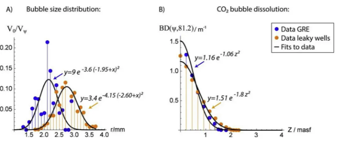
The initial bubble size distribution (ψ), produced during the experiment, was determined from ROV HD images applying the image editing software ImageJ (Farreira and Rasband, 2012). For calibration of bubble sizes, the length of the gas releaser tube (10 cm) was used as scale. Ellipses were manually overlaid to individual bubbles leaving the top of the Ocean Elevator and were marked as overlays. If bubbles had a very irregular shape, they were outlined manually before using the ellipse fitting object of ImageJ. The corresponding bubble volume, V0= 4/3∙π∙req2, was calculated from the equivalent spherical radius, req= (a²∙b)^1/3based on the major, a, and the minor half axes, b, of the fitted ellipse. All determined bubble volumes were added to calculate the total gas volume (Vψ) and the volumetric contribution of each bubble size class (i.e. V0/Vψ), both required to calculate the CO2bubble dissolution rate into seawater during the experiment. The accuracy of bubble size measurements was better than 0.2 mm as determined from the HD image resolution of 55.1 pixels cm⁻¹and a measurement precision of 1 pixel.

Current velocities and directions were recorded during two de- ployments (OCE1 and OCE2) using an Acoustic Doppler Current

Profiler (ADCP, Teledyne RD Instruments) operating at 300 kHz. The vertical resolution of the ADCP was set to 1 m with the first bin starting 3.2 m above the seafloor (masf). OCE1 was a long-term deployment measuring currents over several tidal cycles (i.e. 5 days) that was used to characterize the regional flow field (58.4054 °N, 2.0221 °E) and parameterize the leaky well scenarios, whereas OCE2 was a short-term deployment at the experimental site recording currents 28 m to the east of the Ocean Elevator during the time of the gas release experiment (ADCP measurements during OCE1 and OCE2 can be downloaded from the links:https://doi.pangaea.de/10.1594/PANGAEA.833751,https://

doi.pangaea.de/10.1594/PANGAEA.833761).

The ROV data set including positioning data (longitude, latitude and water depth) was combined with data derived from HydroC-CO2and ADCP measurements by correlating their UTC time stamps. The combined dataset was mapped using the geographic information system software ArcGIS v.10.1 (Fig. 3A). For comparison with numerical pre- dictions, pCO2 data were averaged over periods of equal ROV positioning (i.e. 10 min).

2.2. Gas bubble dissolution model (BDM)

An existing BDM (Vielstädte et al., 2015,2017) was used to calculate the dissolution rate of CO2bubbles in seawater by a single rising gas bubble. The model simulates the shrinking of a gas bubble due to dissolution in the water column, its expansion due to decreasing hydrostatic pressure in the course of its ascent and gas stripping. The BDM uses finite difference methods implemented in the NDSolve object of Mathematica (i.e. LSODA,Sofroniou and Knapp, 2008) solving a set of coupled ordinary differential equations describing these processes for each of the involved gas species (CO₂, N₂, and O₂) and the bubble rise velocity (Wüest et al., 1992). Thermodynamic and transport properties of the gas components, such as molar volume (Duan et al., 1992), gas compressibility (Duan et al., 1992), and gas solubility in seawater (Duan et al., 2006), were calculated from respective equations of state, and empirical equations for diffusion coefficients (Boudreau, 1997), mass transfer coefficients (Zheng and Yapa, 2002), and bubble rise velocities (Wüest et al., 1992), taking into account local pressure, temperature and salinity conditions as measured by CTD casts. A de- tailed description of the model can be found inVielstädte et al., 2015 and2017.

Model boundary conditions and parameterizations (Table 1) were Fig. 2.Gas release experiment (GRE). A) Picture showing the setup of the GRE, i.e. the Ocean Elevator (with yellow syntactic foam blocks) and mounted equipment, deployed at

∼80 m water depth in the vicinity of the Sleipner CO2storage site. B) Single CO2bubble streams were released from the gas release head on top of the Ocean Elevator (in addition Krypton (Kr), used as a tracer gas, was released from the single tube in the back). C) Set-up of the gas control unit, regulating the pressure and gas flow during the experiment.

(4)

obtained from Sea-Bird 9 plus CTD data from July 2012 and run for different initial bubble sizes (r₀) ranging between 1 to 4 mm radius, in accordance to radii observed during the gas release experiment and at North Sea wells leaking methane (Vielstädte et al., 2015). The simulated water depth was defined as 81.8 m in accordance to that of the GRE and depths important for CO2leakage from the seafloor in the Sleipner area. The CO2background concentration in ambient seawater of 0.021 mM (or 434 μatm) was determined from HydroC-pCO2mea- surements at the GRE site prior to the gas release while dissolved O2

concentrations of 0.235 mM were determined at well 15/9-13 (Linke, 2012). Dissolved N2was considered to be in equilibrium with the at- mospheric partial pressure due to a lack of water column measurements.

For a given initial bubble radius (r0), the CO2dissolution rate (R in mol s⁻¹) was determined numerically by the BDM. After numerical computation, R was normalized to the initial bubble CO2content (N0in mol) and divided by the corresponding bubble rise velocity (vb in m s⁻¹) to calculate the normalized bubble dissolution rate (BD in m⁻¹) as a function of the bubble distance from the seafloor (z):

BD r z R r z N v r z m ( , ) ( , )/

( , ) [1 ]

0 b0 0

0

= (1)

Because our experiment and methane leaking wells in the North Sea (Vielstädte et al., 2015) expelled a range of initial bubble sizes, the CO₂ bubble dissolution rate BD (r0,z) was calculated for each initial bubble size and weighted by its volumetric contribution, V0, to the total

emitted gas bubble volume, Vψ.Integrating this weighted bubble dissolution rates over the entire initial bubble size spectrum (ψ) gives the total CO2dissolution rate (BD(ψ,z)) as a function of the bubble distance from the seafloor and with respect to the initial CO2released at the seafloor (Vielstädte et al., 2015,Fig. 4A):

BD z

MI BD r z V V dr

( , ) 1 ( , ) m1

r r

( min ) ( max )

0 0

= (2)

where,r(min)andr(max)are the minimum and maximum bubble sizes of the total spectrum, respectively, andMIis the measurement interval between individual bubble sizes (i.e. 0.1 mm), both determined from HD images of the bubble release.

It should be noted that the applied BDM is valid for the release of single bubble streams but not necessarily for bubble plumes which in- volve additional dynamics (e.g. upwelling of entrained water, bubble rise paths deviating from a straight upward direction). Hence, this study is not meant to capture the physics of overpressure-driven leakage of CO2, such as blowout accidents, which likely involves much larger leakage rates and complex bubble plume dynamics (e.g.,Schneider von Deimling et al., 2015). In this study, the simulation of a single rising bubble seems to be justified because leakage along wells is driven by buoyancy-controlled gas migration (Vielstädte et al., 2015). Enhanced bubble rise velocities have not been observed at methane leaking wells in the North Sea, neither at low nor at high tide (Vielstädte et al., 2015).

This is in contrast to the QICS CO₂ injection experiment, where individual bubbles in Scottish shallow waters rose faster due to bubble Fig. 3.A) Distribution map of pCO2measure- ments (colored circles) during the 4 h ROV observation of the GRE showing the different current flow angles towards the Ocean Elevator (yellow box) when the tide turned and the location of the ADCP (black star) 28 m to the east of the GRE. Background pCO2values (blue dots) were measured upstream of the tidal current before the GRE started (background values measured during the ROV survey when the ROV was not downstream of the CO2plume have been excluded from the plot). B) ADCP measurements of current velocities in eastern (orange dots) and northern (blue dots) directions at 3.2 m above the seafloor during the 4 h ROV observation of the GRE. C) Scheme illus- trating the order (red circles) and magnitude (black values) of pCO2 measurements and down-welling of the CO2plume as measured downstream of the Ocean Elevator.

(5)

plume dynamics (upwelling;Sellami et al., 2015;Dewar et al., 2015).

Due to the larger gas flux in our gas release experiment compared to that observed at methane leaking wells, we cannot explicitly exclude that bubbles rose in the absence of plume dynamics during our experiment (Supplementary video data of our experiment can be downloaded from the link: https://www.pangaea.de/tok/

e3a4d8996affba87b666c04d969672657c32313d). However, we here restrict ourselves by modelling the dissolution rate of a single rising bubble without considering effects like upwelling and entrainment of water due to the overall good agreement of modelling results and data (i.e. measurements of pCO2and the maximum CO2bubble rise height coincide well with modelling results; see Section 3.1.). Other plume dynamics, such as turbulence (Leifer et al., 2015), and/or spiral movement (Schneider von Deimling et al., 2015), which have been observed at other bubble plumes and counter act a reduced bubble dissolution rate induced by upwelling, may explain the good fit of our simulation results to experimental data.

2.3. Plume dispersion model (PDM)

The model uses the COMSOL module “Transport of Diluted Species”

(tds) for chemical species transport via diffusion and advection in a turbulent flow (i.e. Re > 2000 for the North Sea) that is based on the general mass balance equation:

C

t D D C u C S mol

([ M T] ) [m s3 ]

= + + (3)

where,Cis the concentration of the dissolved species (here dissolved inorganic carbon (DIC) in mol m⁻³),tis the time (s), the Nabla operator

∇refers to the derivatives with respect to the spatial coordinates x,y, and z, uis the current velocity vector (m s^-1),Ddenotes the diffusion coefficient including a molecular (DM) and a turbulent diffusion component (DT) (m²s^-1), andSis the source term of DIC production (mol m⁻³ s^-1) resulting from CO2 bubble dissolution expressed as 2-D Gaussian distribution:

S we R BD z mol

m s

1 ( , )[ ]

x y w

CO

( )

2 3

2 2

=

+

(4) where,wdenotes the area (m²) of the Gaussian pulse in x and y direction,RCO2is the rate of CO2gas bubble release (mol s⁻¹) from the seafloor, andBD(ψ,z)is the normalized rate of CO2bubble dissolution as determined from the BDM (Eq.(2),Fig. 4B).

Table 1

Parameterization of the bubble dissolution model.

Parameter values/Equations Range Variance Reference

aDiffusion coeff.: Di/ m²s⁻¹

DO2= 1.05667∙10⁻⁹+4.24∙10^-11∙T T:0-25 °C 1.00∙10⁻²¹ Boudreau, 1997

DN2= 8.73762∙10⁻¹⁰+3.92857∙10^-11∙T T:0-25 °C 2.94∙10⁻²³ Boudreau, 1997

DCO2= 8.38952∙10⁻¹⁰+3.8057∙10^-11∙T T:0-25 °C 4.76∙10⁻²⁵ Boudreau, 1997

Mass transfer coefficient: KL,i/ m s⁻¹

KL= 0.013∙ (vb10²/(0.45 + 0.4∙r∙10²))^0.5∙Di0.5 r ≤ 2.5 mm Zheng and Yapa, 2002

KL= 0.065∙Di0.5 2.5 < r ≤ 6.5 mm Zheng and Yapa, 2002

KL= 0.0694 (2∙r ∙10²)^−0.25∙Di0.5 r < 6.5 mm Zheng and Yapa, 2002

Fit to CTD data as function of the water depth (zsw)

T(zsw) = 8 + 7/(1+e0.375 (−21.7512+ zsw)) [°C] Zsw: 0-100 m 3.99∙10⁻² CE12010 45-CTD12

S(zsw) = 35.12-0.67/(1+e0.4125 (−20.1595+ zsw)) [PSU] Zsw: 0-100 m 4.97∙10⁻⁴ CE12010 45-CTD12

Density of sea water: φSW/ kg m⁻³ φSW(zsw) = 1027.7-2.150/

(1+e0.279 (−21.612+zsw)) Zsw: 0-100 m 6.8∙10⁻³ Unesco, 1981

Bubble rise velocity: vb / m s⁻¹

vb= 4474∙r^1.357 r < 0.7 mm Wüest et al., 1992

vb= 0.23 0.7 ≤ r < 5.1 mm Wüest et al., 1992

vb= 4.202∙r^0.547 r ≥ 5.1 mm Wüest et al., 1992

Gas solubility: ci/ mM

cN2= 0.622 + 0.0721∙zsw Zsw:0-100 m 2.5∙10⁻³ Mao and Duan, 2006

cO2= 1.08 + 0.1428∙zsw Zsw:0-100 m 9.8∙10⁻³ Geng and Duan, 2010

cCO2=(0.041 + 0.00476∙zsw) ∙ φSW Zsw:0-100 m 5.7∙10⁻⁵ Duan et al., 2006

CO2molar volume: MVCO2/ L mol⁻¹

MVCO2= 1/(0.04 + 0.00458∙zsw) Zsw:0-100 m 0.1 Duan et al., 1992

Hydrostatic Pressure: Phydro/ bar Phydro= 1.013+φSW∙g∙zsw

a The parameterization of the diffusion coefficients is based on a seawater salinity of 35. Pressure effects have been neglected because the resulting error is < 1%

at < 100 m water depth.

Fig. 4.A) Bubble size distributions measured during the GRE (blue dots) and at methane leaking wells in the CNS (orange dots, Vielstädte et al., 2015). B) Calculated rates of CO2bubble dissolution as a function of the distance to the seafloor (z) based on the initial bubble size distributions of the GRE (blue dots) and leaking wells in the CNS (orange dots).

CO2bubbles dissolve within the lower 2 m of the water column. Details on the accuracy of data fits (black line) are given in the Supple- mentary Material.

(6)

The horizontal advective flow (u) in x and y direction is parameterized according to least-squares fits to ADCP velocity data measured at 3.2 masf and applying the Kármán–Prandtl “Law of the Wall”

(LOW) describing the current velocity vector as a function of time (t) and distance from the seabed (z) (e.g.McGinnis et al., 2014):

u t z_x( , ) ^{u t}^x_ka^*^{( )}ln( ), [ ]_z^z ^m_s

= 0 (5)

u t z u t ka

z ( , ) ( ) z

ln( )

y y*

0

=

Where,u^*denotes the shear velocity in x and y direction calculated from ADCP data,z0is the roughness length (1.4∙10⁻⁴m for the North Sea;McGinnis et al., 2014) defining the height at which the current velocity tends to zero (Lefebvre et al., 2011),zis the distance to the seafloor, andkais the dimensionless Kármán constant (0.4,Kundu and Cohen, 2008). As such, advective velocities are assumed to be hor- izontally, but not vertically and temporarily uniform. The vertical advection component is ignored because it is orders of magnitude smaller than the horizontal one.

Since the model uses least-squares fits to ADCP velocity data, small- scale fluctuations (eddies) in the turbulent flow are not explicitly resolved. The convective phenomenon of turbulent mixing is accounted for in the calculation of the species transport by using an added component of diffusion (DT), which is expressed in dependency to z, ka and ur*,the shear velocity in resultant current direction (e.g.McGinnis et al., 2014):

D ka u z m

T r* s2

= (6)

Molecular diffusion (DM) is calculated according to Boudreau (1997)as a function of temperature, pressure, and salinity and is on the order of 10⁻⁹m²s^-1. Diffusion is assumed to be isotropic and hence, is the only mechanism transporting dissolved species vertically in the model domain. Equations and parameter values are provided inTables 2 and 3for the GRE and leaky well simulation settings, respectively.

To avoid numerical instabilities of the solution in the advection dominated leakage scenario, the COMSOL Model uses both, streamline- upwind (Galerkin method (SUPG),Do Carmo and Alvarez, 2003) and crosswind (Codina, 1998) stabilizing advection schemes, which add artificial diffusion in streamline and orthogonal direction to the advection vector of the advection-diffusion equation (Eq. 3). Numerical diffusivity was limited by defining a lower gradient limit (glimin mol m⁻⁴) denoting the smallest concentration change across an element that is considered by stabilization. glim was defined as 3 mol m^-3 weighted by the mesh element size (h) and has been determined from sensitivity analysis, i.e. increase ofg_limuntil the solution remains constant (numerical accuracy) while also ensuring sufficient numerical stability. The combination of using stabilizing advection schemes and a high-resolution non-uniform mesh including a local mesh refinement around the gas release where concentration gradients change rapidly ensured the model is well suited for maintaining sharp concentration

gradients while also ensuring sufficient numerical stability. None- theless, with the finite element stabilization method the tracer dispersion calculated by the model is somewhat enhanced by the artificial diffusion that was added to the model to obtain numerically stable results.

The time-dependent problem was solved by integration of the partial differential equation (i.e. Eq.(3)) in time according to the implicit backwards differentiated formula method of COMSOL Multiphysics (Press et al., 2007). The COMSOL Multiphysics solver automatically chooses appropriate numerical time steps which were set to be within a certain relative tolerance (i.e. 0.01) for the accuracy of the integration estimated during runtime (Press et al., 2007). The numerical performance (stability) was controlled after each model run by mass balance error (MBE) calculations, which were overall better than 2%.

The computed concentration of DIC, which is the sum of chemical species resulting when CO₂ dissolves in seawater ([CO₂]+[HCO₃⁻] +[CO32-]), is converted into carbonate system parameters of interest, i.e. pCO2 and pH, applying an analytical solution (Zeebe and Wolf- Gladrow, 2001) assuming constant total alkalinity (TA) and applying physical parameter values (temperature, salinity, and pressure) obtained by CTD casts (Sea Bird 9 Plus) in July 2012 (Table 4). Total alkalinity of seawater was determined by titration with 0.02 N HCl using a mixture of methyl red and methylene blue as indicator. The titration vessel was bubbled with argon to strip any CO2 produced during the titration. The IAPSO seawater standard was used for calibration; analytical precision and accuracy are both ∼2%. TA is assumed to be constant during the GRE.

2.4. Simulating the gas release experiment

The first modelling case is designed to simulate the GRE over the 4 h period of ROV observation, for which the effects of the tidal turn on CO2

dispersion are examined and compared toin situ pCO2measurements.

The computational domain is set to be 50 × 50 × 20 m³, with a smaller rectangle (2.2 × 0.7 × 2.2 m³) in its center, which represents the geometry of the Ocean Elevator from which the CO2bubbles are released.

The non-uniform finite element mesh has a spatial resolution of 0.075–1.75 m, with a finer element distribution of maximal 0.2 m in size around the gas release spot (further information on the model setup is given in the supplementary material).

The DIC source rate (S), resulting from vertical CO2 bubble dissolution, is parameterized according to the preset gas flow (RCO2) of 85 kg day⁻¹of CO2and the calculated bubble dissolution rate (BD) of the initial bubble size distribution (ψwith a peak radius of 2.1 mm) at a water depth of 81.8 m and ambient seawater conditions (Table 2).

In contrast to the plume dispersion model setup, where the current velocity is parameterized in the model domain according to ADCP measurements and the LOW towards the seabed, current velocities (and other convective parameters) around the Ocean Elevator were calculated numerically because the ADCP was deployed too far away (i.e.

28 m) from the experiment to resolve modifications in the turbulent flow that the obstacle of the Ocean Elevator induced. Generally, the Table 2

Parameterization of the plume dispersion model for the GRE simulation setting.

GRE Parameter Parameter values/Equations Unit

*Resultant velocity as a function of time (t) in seconds u t_r( ) 120 0.0062t 36Sin( ^t)

= + 8000 mm s⁻¹

Sand roughness height kseq=3.2 μm

Turbulent intensity I_T=0.05

Turbulent length scale LT=0.01 m

*Rate of CO2bubble dissolution BD( _GRE, 81.2)=IF z[ <2.21, 0, 7.6e^{0.31 2}^z] m⁻¹

Leakage rate RCO2= 31 t yr⁻¹

Area of the Gaussian pulse w= 0.3 m²

* Details on the accuracy of data fits and the correlation of fit parameters are provided in the supplementary material.

(7)

flow field behind an obstacle is suppressed and forms periodically swirling vortices. These effects were resolved by using a k-εturbulence model implemented in COMSOL Multiphysics (i.e. the spf physics interface) which calculates the turbulent fluid flow numerically by solving the Reynolds-Averaged-Navier-Stokes-Equation (RANS).

Using the k-εturbulence model, the advective flow acts in the direction of the Reynolds-averaged velocity and not in that of the real

instantaneous velocity of the fluid in the field. As a result, small eddies of the turbulent flow are not explicitly resolved, having however, a pronounced effect on the species transport, as they cause additional mixing. Turbulent mixing is accounted for in the calculation of the species transport by using an added component of diffusion (DT in addition to molecular diffusion) that is equal to the ratio of the turbulent kinematic viscosityvT(m²s⁻¹) to the dimensionless turbulent Table 3

Parameterization of the plume dispersion model for the leaky well simulations.

Parameter Parameter values/Equations

*East velocity (m s⁻¹) as a function of time (t) and depth (z) above the seafloor

u t z_x( , ) Log[ ]

Sin t

ka

z z

0.37 2.21 ( 5279)

22400

= 0

+

*North velocity (m s⁻¹) as a function of time (t) and depth (z) above the seafloor

u t z_y( , ) Log[ ]

Sin t

ka

z z

2.52 3.94 ( 36019)

22400

= 0

*Shear velocity (mm s⁻¹) at 3.2 masf as a function of time (t)

( ) ( )

u t_r^*( )= 2.05+4.56^Sin^[ ₂₂₄₀₀⁽^t⁺^8065)] ²+ 1.84+0.65^Sin ^[₂₂₄₀₀⁽^t⁺^23260)] ²

Turbulent diffusion coefficient (m²s⁻¹) D t zT( , )=ka u tr*( ) 103z

Molecular diffusion coefficient (m²s⁻¹) D_M( )t =10 ⁹

Roughness length (m) z0=1.4 104(e.g.McGinnis et al., 2014)

Kármán constant ka=0.4(Kundu and Cohen, 2008)

*Normalized rate of CO2bubble dissolution (m⁻¹) BD z( )=1.16e ^1.06^z²

Leakage rate of CO2(t yr⁻¹) RCO2= 10, 20, 55

Area of the Gaussian pulse (m²) w = 0.5

* Details on the accuracy of data fits and the correlation of fit parameters are provided in the supplementary material.

Table 4

Parameterization of the carbonate system sub-model.

Carbonate system

parameters Parameter values/Equations Source

Total alkalinity (TA) /

mM 2.333 CE12010 45-CTD12

BackgroundpCO2*/

μatm 434 CE12010 44-HydroC;

https://doi.pangaea.

de/10.1594/

PANGAEA.899480 Background DIC

(DIC0)/ mmol kg^–1

2.115 Calculated from TA&

pCO2*

Background pH* 8.0 Calculated from TA&

pCO2* Seawater

temperature/ °C 7.8 CE12010 45-CTD12;

de/10.1594/

PANGAEA.823042 Seawater salinity/

PSU 35.18 CE12010 45-CTD12;

de/10.1594/

PANGAEA.823042

Water depth/ m 81.8 CE12010 44-ROV

Total sulfide/ mM 0 Total boron/ mM 0.42 Dissolved Ca ions/

mM 11.4

Spatial DIC heterogeneity/

μM

16 or 0.7 g/m³excess CO2 DIC bottom water

concentrations in Tommeliten seepage Seasonal DIC area

variability/ μM 60 or 2.64 g/m³excess CO2 Variability based on

upper DIC bound given inBozec et al.

(2006)and lower bound measured in the Sleipner area (DIC0)

aConversion of excess DIC (μM) inpCO2

(μatm)

pCO e DIC DIC

e DIC DIC DIC

1/(1 ) (430 4 0.03 )

1/(1 ) (480 2.1 0.03 0.00016 )

DICex ex ex

DICex ex ex ex

2 50 2

50 2 3

= + +

+ + + +

Fit to model-derived data (valid up to DICexof 1000 μM) Details on the accuracy of data fits and the correlation of fit parameters are provided in the supplementary material.

(8)

Schmidt numberScT:

D v

Sc m

T T s

T

= 2

(7) WhereScTis a model constant with a typical value of 0.71 (Gualtieri et al., 2017), andv_Tis calculated numerically based on the turbulent kinetic energy (kin m²s⁻²) and the dissipation rate of turbulent kinetic energy (εin m²s^-3) determined by the k-εturbulence model:

v c k m

[ s ]

T µ

2 2

= (8)

where cμis a dimensionless model constant (i.e. 0.09; Launder and Spalding, 1974). Using the k-εturbulence model, turbulent velocities (u), viscosities (vT) and diffusivities (DT) are calculated numerically, based on a transfer function of the measured current velocity magnitude (i.e. least- squares fit to the velocity data at 3.2 masf during OCE2) and algebraically specified mixing length (LT) and turbulent intensity (IT) defined as inlet boundary condition (Table 2). By defining an equivalent sand roughness height (kseq) of 3.2 μm at the seafloor, which is related to the roughness length (z0) by z0=kseq/30 (Lefebvre et al., 2011), the non-slip boundary condition at the bottom of the model domain accounts for friction at the seabed and the resulting decline in average flow velocity towards the seabed.

The spread of dissolved CO2during the experiment was obtained from coupling the physics interface of mass transport (tds) to the k-ε turbulence model (i.e. the spf physics interface), thus, accounting for modifications in the advective and diffusive phenomena that the obstacle of the Ocean Elevator induced.

To significantly lower the computational requirements when solving for the turbulent flow and mass transport during the tidal turn (e.g.

avoiding too many open boundaries that are weakly constrained), the effect of the tidal currents passing the Ocean Elevator geometry was simulated by rotating the obstacle in the model domain relative to a constant flow direction (defined as normal velocity condition at the inlet boundary). The outflow boundary in streamline direction is set as a zero-gradient condition, which accounts for advective mass transfer but neglects any diffusive fluxes across the boundary. The remaining boundaries are defined as slip, no-flow boundary conditions with no- friction, no-viscous forces, and no-mass transfer for seawater or dissolved species. The angles between the current flow and the Ocean Elevator during the tidal turn were calculated by correlating UTC time stamps of ADCP data (i.e. resultant current direction), and ROV position and heading duringpCO2measurements. Based on the spatial orienta- tion of the Ocean Elevator, whose long side was heading 40° to the north-east, two rotation angles of 40° and 70° were determined, in which most of the HydroC-pCO2measurements occurred and for which the simulations were run.

Initial DIC concentrations and current velocities in the model domain are prescribed to be zero, so that the model calculates excess DIC concentration relative to the background signal observed in the field (Table 4). After proving sufficient model stability by mass balance error calculations, model results were evaluated against averaged pCO2

measurements (Fig. 5B) in order to fit the turbulent parameters (turbulent length scale and turbulent intensity) and validate the model for further application of the leaky well scenarios.

2.5. Simulating CO2leakage from a well

The second modelling case is designed to simulate a range of hypothetic, but realistic scenarios of CO2release along an abandoned well from the Sleipner CO2storage site into the North Sea, using site-specific current velocity data (Fig. 6) as well as initial bubble sizes (Fig. 4A) and gas flows found at methane-leaking wells in the vicinity (Vielstädte et al., 2015). The computational domain is set to be 600 × 600 × 20 m³ with the point-source (∼ 4 m²) CO₂leak located at the seafloor in the model center. The non-uniform mesh has a spatial resolution of

0.15–3 m with a higher finite element density about 80 m around the gas release spot.

Based on gas emissions measured at methane-leaking wells (Vielstädte et al., 2015), we define possible leakage rates (RCO2) of 10, 20, and 55 t yr⁻¹of CO2. The advective flow (u) is prescribed from least-squares fits to 12-h time-series data of current velocities in east (x) and north (y) directions (OCE1 Bin1) considering the velocity decrease towards the seabed induced by friction(Eq.(5),Table 3).

The chosen 12-h time-series data was found to be representative for a whole tidal cycle because the North Sea has a semi-diurnal tide (Fig. 6A). The model accounts for friction at the seabed, so that the advective flow and the turbulent diffusivity are assumed to be hor- izontally, but not vertically and temporarily uniform.

Four open lateral boundaries with a zero-gradient boundary condition allow for convective flow in and out of the model domain, while any diffusive fluxes are neglected. The lower and upper boundaries at the seafloor and towards the sea surface are set to no-flow conditions, i.e. no-mass transfer permitted; no gas exchange with the atmosphere considered. Initial DIC concentrations and current velocities in the model domain are prescribed to be zero, so that the model calculates excess DIC concentration relative to the background signal observed in the field. To ensure mass balance, the computational domain is tested to be sufficiently large to avoid that plumes of dissolved CO2leaving the model domain may return through the boundaries within the simulated time span.

3. Results and discussions 3.1. The gas release experiment

ROV video observation revealed moderate gas bubbling on top of the Ocean Elevator (Fig. 2). In total, 18 single CO2bubble streams with initial bubble sizes of 1.3 to 2.9 mm in radius (Fig. 4A) were emanating from the release head and reached a final rise height of ∼2 m. This is consistent withpCO2 measurements which did not exceed the local background value (∼430 μatm) two meters above the release spot (Fig. 3C).

Rapid CO2bubble dissolution into seawater significantly increased the bottom water partial pressure of CO₂close to the release site to values of 2327 μatm (3 m downstream of the release,Fig. 3C). How- ever, elevatedpCO2levels were only observed in a very narrow band (< 1 m width) of water mass downstream of the Ocean Elevator. As a result of quick dispersion by ambient bottom currents, background values were attained already ∼30 m downstream of the artificial leak, indicating that the impact of the experiment was limited to near-bottom waters and a rather small distance of a few tens of meters downstream of the leak (Fig. 3). This observation is in line with the QICS CO2in- jection experiment, where the CO2concentration away from the injection site was undetectably small and the detectable signal was con- fined to a small area in the vicinity of the injection point (Mori et al., 2015;Blackford et al., 2014).

Although the experiment successfully simulated CO₂leakage into the North Sea at low rates, the physical response in the dynamic water column was quite complex. The numerical model successfully simulated the suppressed pressure and advective flow downstream of the Ocean Elevator, which induced a downwelling of the solute CO2 plume (Fig. 5A). This effect was particularly strong at the beginning of the experiment, when the turbulent flow was heading towards the long side of the Ocean Elevator (Figs.3A,5A). During our experiment the density increase of water masses caused by CO2dissolution has no considerable effect on the observed down-welling because the maximumpCO2value recorded induces an increase in seawater density of < 0.001 kg m⁻³ (Duan et al., 1992,2006). However, for larger leakage rates the density effect will become more important.

According to numerical results, the turbulent diffusion coefficient varied in the order of 10⁻⁴to 10^-7m²s^-1during the experiment. Low

(9)

turbulent diffusivities occurred close to the seafloor and downstream of the Ocean Elevator in the region of slow advective flow (Fig. 5A). Thus, it is evident that the experimental setup not only significantly decreased the horizontal advective transport, but also suppressed the turbulent

mixing of the CO2plume downstream of the Ocean Elevator.

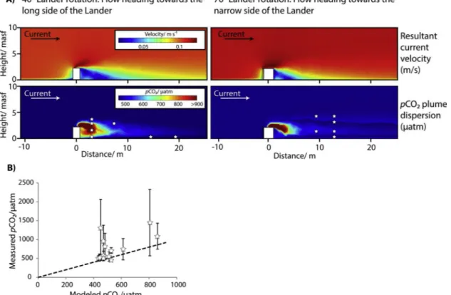
Evaluation of the numerical results against pCO2 measurements reveals that the applied numerical models accurately describe the rapid CO2 bubble dissolution in seawater and the spatial and temporal Fig. 5.A) COMSOL model results of the GRE simulation showing the modified current velocity field (top) and the dispersion of the solute CO2plume (bottom) downstream of the Ocean Elevator/Lander (white box) for the two simulated rotation angles of the Lander relative to a normal flow vector (black and white arrow).

B) Comparison ofpCO2measurements and model-derivedpCO2values for each ROV measuring position (white stars) indicating that the COMSOL model under- estimates measured values but is in the scatter of most measurements. Model-derivedpCO2values bear an uncertainty of ± 124.5 μatm as determined from the standard deviation (1σ) of the least-squares data fit that was used in the model to convert DIC concentrations intopCO2data (seeTable 4). The 1:1 line of model- derivedpCO2values and HydroC-pCO2measurements is indicated by the dashed line.

Fig. 6.A) ADCP velocity data in north (blue), east (orange), and resultant (red) current direction measured 3.2 m above the seafloor during the OCE1 long-term deployment of the ADCP. Data show a tidal asymmetry, referring to differences in the ebb and flood current velocities, i.e. stronger currents during high tide (HT) than during low tide (LT) and weaker currents during high slack water (HSW) than during low slack water (LSW). B) Scheme il- lustrating the Law of the Wall (LOW), where the current flow (dark red) and turbulence (dark blue) increase with distance to the seafloor, which results in the weakest dispersion of the CO2plume at the seafloor. Together with the declining rate of CO2 dissolution during bubble ascent, this causes the largest CO2

footprints (pink line) to occur at the seabed.

Figures C) and D) show current velocities and turbulent diffusivities, respectively, calculated by application of the LOW in the lower 3.2 m of the water column. The first 12 h of the velocity/turbulence data set were employed for the leaky well scenarios (area shaded in light blue).

(10)

dynamics of excess CO2 in a tidal flow (Figs. 4B,5A). In situmeasurements of the spatialpCO2dispersion correspond well to numerical simulations, showing that bubbles are depleted in CO2 1.9 m above their release (Fig. 4B) and the added CO2is diluted quickly in ambient bottom waters (Fig. 5A). Nonetheless, the model tends to underestimate pCO2values measured in the field as the modeled values cluster in the lower range of thepCO2measurements (Fig. 5B). Possible explanations for this deviation are 1) short-term fluctuations in the real advective flow, which have not been considered in the model, 2) the influence of the ROV and its thrusters on the current flow, also not considered in the model, and 3) numerical diffusivity introduced to the model.

One simplification in the model is that the advective flow acts in the direction of the Reynolds-averaged velocity and not in the real instantaneous direction of the current velocity in the field, where abrupt changes in the flow direction might have resulted in patches of high pCO₂waters that separated from the main plume, and thus, shortly increasedpCO2signals measured in the field. The effect of short-term fluctuations is consistent with the large scatter ( ± 25% on average) in pCO2 measurements for each measuring position (Fig. 5B). Further- more, as the HydroC-pCO2sensor was attached to the front porch of the ROV,pCO2measurements were likely influenced by the obstacle when the plume hits the ROV (similar to the effect of the Ocean Elevator).

Unphysical, numerical diffusivity, which would also result in an un- derestimation of measuredpCO2values, has been minimized by tuning the lower concentration gradient limit (glim) for artificial diffusion, but may have influenced our simulations.

Despite these simplifications described above, the model captures the main features of the data; i.e. rapid bubble dissolution, quick dispersion, narrow width of the plume, and the downwelling of the plume leeward of the obstacle. We therefore argue that the applied models are sufficiently reliable to predict solute plume dispersion in the near field of a small CO₂leak. Nonetheless, it should be noted that limitations to our modelling are related to bubble plumes and gas bubbles coated with surfactants, which physics have not been considered in our numerical simulations.

3.2. The leaky well scenarios

The simulated leaky well scenarios (Fig. 6) with constant and continuous CO2leakage of 10, 20 and 55 t yr⁻¹, respectively, resulted in dynamic plumes of acidified bottom water that were quickly dispersed from the source location. Generally, within a distance of less than 120 m from the leak, backgroundpCO2levels are predicted (Fig. 7A). As expected, the magnitude of seawater acidification and the spatial extent of detectable CO2 plumes at the seafloor increased with increasing leakage rates. The strongest acidification was found for the high emission scenario (55 t yr⁻¹) at high slack water (HSW) when the bottom water pH value dropped significantly from a background of 8.0 to less than 6.0. (Fig. 7C).

The simulated initial bubble size distribution with a peak radius of 2.6 mm (Vielstädte et al., 2015) loses its CO2almost completely within the lower 2 m of the water column. 80% of its initial CO₂content is already dissolved within the first meter above the seafloor (Fig. 4B).

Such rapid CO2bubble dissolution causes leaking CO2to remain in the bottom waters and inhibits direct bubble transport into the atmosphere.

This is in line with our experimental results and other recent studies (Hvidevold et al., 2015;Dewar et al., 2013;Dissanayake et al., 2012;

Phelps et al., 2014; Kano et al., 2010). However, once a leak occurs, some of the dissolved CO2may ultimately reach the atmosphere via diffusive sea-air gas exchange, mostly depending on the mixing of the water column and the water depth at which leakage were to occur (Phelps et al., 2014).

In the following, we discuss key drivers controlling the dispersion of CO2emitted at a point source in a tidally influenced oceanic setting (section3.2.1), before discussing modelling-derived estimates on the spatial footprints of potentially harmful and detectable CO2plumes in

seawater in order to support risk assessments (section 3.2.2) and monitoring strategies (section3.2.3) of offshore CO2storage sites, respectively. Finally, we discuss the propensity of wells to leak at Sleipner (section3.2.4).

3.2.1. CO2plume dispersion and relationship with tides

Using the tidal velocity data of July 12^th2012 for the CNS (Fig. 6A), our leaky well simulations show a strong correlation between the dispersion of the dissolved CO2plume in the water column and the phase of the semi-diurnal tides (Fig. 7). Common temporal and spatial features include (1) the accumulation of DIC near the leak during periods of decelerating flow, (2) thin elongated plumes with low DIC concentrations during periods of strong unidirectional flow, (3) wider plume shapes when the tides turn, and (4) extensive build-up of DIC peak concentrations during slack water periods with low or stagnant flow (which is in line with other recent studies, e.g.Greenwood et al., 2015,Fig. 7A).

These observations indicate that continuous CO2leakage into the North Sea would result in a series of plume concentrations and shapes during a tidal cycle, with peak concentrations and largest plume footprints occurring around slack water periods and close to the seafloor, where advective and diffusive fluxes are low (Fig. 6). In contrast, at stronger flow DIC concentrations should be efficiently diluted with ambient seawater quickly reaching background values.

Higher simulated DIC concentrations during low tide (LT) as compared to high tide (HT) were primarily a consequence of the measured tidal asymmetry, referring to differences in the ebb and flood current velocities (Figs. 6A,7C). Tides may not only affect CO2dispersion but also the CO₂emission rate at the seabed since studies at natural gas seeps (e.g. Leifer and Wilson, 2007;Linke et al., 2010;Tryon et al., 1999; Wiggins et al., 2015) and the QICS CO2 injection experiment (Blackford et al., 2014) imply that rates of bubble release at the seafloor respond to tidal pressure fluctuations.

Calculated turbulent diffusion coefficients (DT) were in agreement to those measured in the benthic boundary layer of permeable sedi- ments in the Central North Sea (McGinnis et al., 2014), suggesting that the applied correlation ofDTand measured current velocities (Eq.(6)) yielded realistic results. In our simulations, DT at 3.2 m above the seabed varied between 2 ∙ 10⁻³m²s^-1at minimum and 9 ∙ 10⁻³m²s^-1 at maximum current flow velocity. It was significantly smaller, that is on the order of 10^-7m²s^-1, close to the seafloor (0.01 masf) throughout the whole tidal cycle (Fig. 6D). Despite the wide range of diffusion coefficients, the dimensionless Péclet number (Pe), that is the ratio of the rate of tracer advection to the rate of tracer diffusion, was always larger than 10 - an indication that diffusive fluxes were overall negligible. This implies that for a North Sea setting and at small scales lateral diffusive fluxes are low and thus, have only a negligible effect on the dispersion of the dissolved CO2plume, whereas the advective transport (i.e. tidal current) is a key parameter. It should however be noted, that diffusion was the only mechanism that controlled the vertical dispersion of the CO2plume in our three leaky well simulations, as we neglected any vertical advective transport.

3.2.2. Environmental impact of a CO2-leaking well in the CNS

The environmental impact of CO₂leakage into seawater is a critical issue in risk assessment studies and depends on the magnitude of seawater acidification and the spatial and temporal extent of any potentially harmful pH reductions exceeding a site-specific natural variability, which marine biota should be adapted to. In the deeper layers of the Northern and Central North Sea marine DIC concentration varying between 2.11 and 2.17 mmol kg⁻¹have been observed (Bozec et al., 2006). This corresponds to a seasonal variability in pH of 7.85–8.02, assuming a constant TA of 2.333 meq. dm^-3(a simplification due to lacking literature data on seasonal variations in TA in North Sea bottom waters) and physicochemical seawater conditions as measured in the Sleipner area in July 2012 (T = 7.8 °C; S = 35.18, P = 9.2 bar;