Supplementary material for:Footprint and detectability of a well leaking CO

(1)

Supplementary material for:

Footprint and detectability of a well leaking CO

2

in the Central North Sea: Implications from a field experiment and numerical

modelling

Lisa Vielstädte, Peter Linke, Mark Schmidt, Stefan Sommer, Matthias Haeckel, Malte Braack, Klaus Wallmann

1

2

3

4

5

6 7

8

9

(2)

All data were processed using least-squares fitting tool implemented in the Wolfram Mathematica software. In the following, the accuracy of applied fit equations and the correlation of fit parameters are provided in table form.

1.1 Velocity data

Table S1: Fitting velocity data in north direction (uy in mm s^-1) as a function of time (t/ s) and distance to the seafloor (z; here 3.2 m) by application of the low of the wall (with z0=1.4 10∙ ^-4 m and ka=0.4; e.g.

McGinnis et al., 2014). This fit has been used to force the horizontal advective transport of DIC in the leaky well simulations.

u

_y(

t , z

)=

( ^{a−b ∙}

^sin

[ ^{π ∙}

²²⁴⁰⁰^(t⁺

^c) ])

ka ∙

log[3.2

z

₀ ]

Correlation matrix for parameters Least squares estimates of parameters Standard error

a b c (1-σ)

a 1 0.04 0.03 -2.52 0.03

b 0.04 1 0.03 -3.94 0.04

c 0.03 0.03 1 36019 79

Standard deviation of the fit (1σ)/ mm s^-1 29.7

For data fitting, ADCP velocity data recorded during OCE1 Bin 1 (3.2 masf) have been used.

Table S2: Fitting velocity data in east direction (ux in mm s^-1) as a function of time (t/ s) and distance to the seafloor (z; here 3.2 m) by application of the low of the wall (with z0=1.4∙10^-4 m and ka=0.4; e.g.

McGinnis et al., 2014). This fit has been used to force the horizontal advective transport of DIC in the 11

12 13 14 15

16

(3)

17 18

(4)

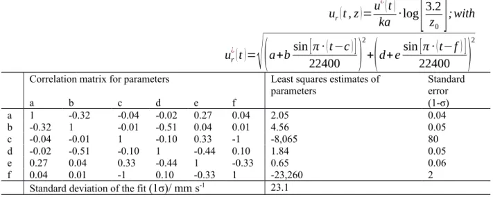
from the seafloor by application of the low of the wall. The fit has been used to calculate the shear velocity (

u

_r^¿ in mm s^-1) as a function of time (t in s) in order to further determine the water column turbulent diffusivity (DT), which has been used to force the turbulent diffusive transport of DIC in the leaky well simulations.

u

_r(

t , z)= u

^¿(

t

)

ka ∙log [

^3.2

^z

⁰

] ^;with

u

_r^¿(t)=

√ ⁽ ^a+ ^b

^sin²²⁴⁰⁰

^[ ^{π ∙}

⁽

^t

^−c⁾

^] ⁾

²⁺

⁽ ^d+ ^e

^sin²²⁴⁰⁰

^[ ^{π ∙}

^(t−

^f

⁾

^] ⁾

²

Correlation matrix for parameters Least squares estimates of

parameters Standard

error

a b c d e f (1-σ)

a 1 -0.32 -0.04 -0.02 0.27 0.04 2.05 0.04

b -0.32 1 -0.01 -0.51 0.04 0.01 4.56 0.05

c -0.04 -0.01 1 -0.10 0.33 -1 -8,065 80

d -0.02 -0.51 -0.10 1 -0.44 0.10 1.84 0.05

e 0.27 0.04 0.33 -0.44 1 -0.33 0.65 0.06

f 0.04 0.01 -1 0.10 -0.33 1 -23,260 2

Table S4: Fitting resultant velocity data (ur in mm s^-1) as a function of time (t in s) at 3.2 m distance from the seafloor. The fit has been used as velocity condition at the inlet boundary of the GRE model, constraining the numerically-derived advective flow during the experiment.

u

_r(

t ,

3.2)=a+b ∙ t+

c ∙

sin(

π ∙ t

8000)

a b c (1-σ)

a 1 -0.95 -0.80 120 4

b -0.95 1 0.83 0.0062 0.0006

c -0.80 0.83 1 -36 3

19

(5)

1.2 Carbonate system parameters

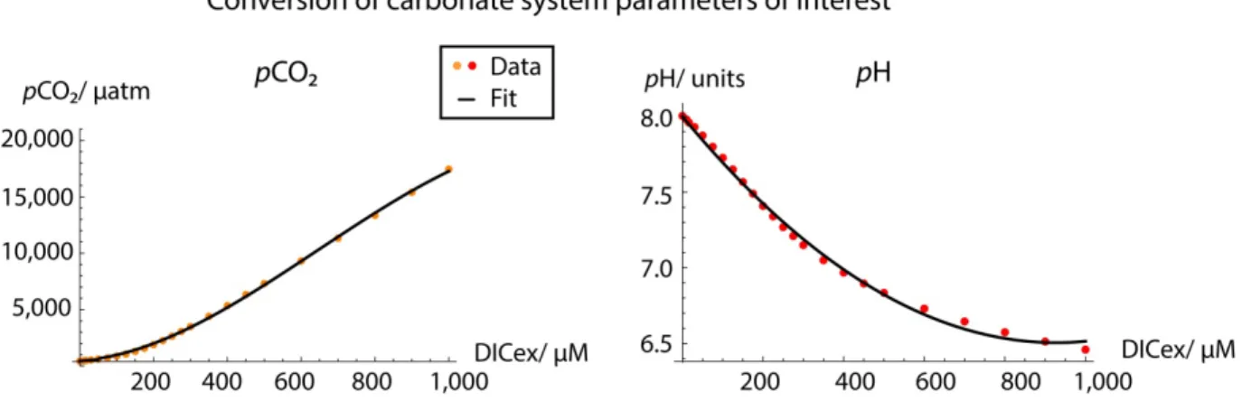
Table S5: pCO2 signals (µatm) derived from applying an analytical solution were fitted as a function of DIC excess concentration (DICex in µM) assuming constant TA. This transfer function has been used to convert computed DICex concentrations into pCO2 signals in order to compare results of the GRE plume dispersion model with pCO2 signals observed in the field.

pCO

₂=1/ (1+

e

^DIC^ex⁻⁵⁰)∙

(

430+a ∙ DIC_ex+b ∙ DIC_ex²

)

⁺^1/(1+

^e

^50−DIC^ex⁾

^∙ (

⁴⁸⁰⁺

^{c ∙ DIC}

ex+d ∙ DIC_ex²+f ∙ DIC_ex³

)

a b c d f (1-σ)

a 1 -0.93 0.03 -0.03 0.03 3.9 8

b -0.93 1 -0.05 0.05 -0.04 -0.03 0.2

c 0.03 -0.04 1 -0.95 -0.89 2.1 0.4

d -0.03 0.05 -0.95 1 -0.98 0.030 0.001

f 0.03 -0.04 0.89 -0.98 1 -1.6 ∙ 10^-5 1.0 ∙ 10^-6

Standard deviation of the fit (1σ)/ µatm 124.5

For data fitting, pCO2 data predicted by an analytical solution have been used (details on the parameterization of the sub-model are given in Tab. 4).

Table S6: pH levels derived from applying an analytical solution were calculated as a function of DIC excess concentration (DICex in µM) assuming constant TA. This transfer function has been used to covert modeled DICex concentrations in pH units in order to evaluate the environmental impact of the three leaky well scenarios.

pH=8+ a∙ DIC

ex+

b ∙ DIC

ex2

a b (1-σ)

a 1 0.96 0.00321 0.00005

b 0.96 1 1.73 ∙ 10^-6 7.0 ∙ 10^-8

Standard deviation of the fit (1σ)/ units 0.03

For data fitting, pH data predicted by a carbonate system sub-model have been used (details on the parameterization of the sub-model are given in Tab. 4).

21 22

23

24

(6)

concentration and the applied data fit (black curve) in order to convert plume model-derived DIC excess concentrations into carbonate system parameters of interest.

1.3 Initial bubble size distributions

Table S7: Fit function to calculate the dimensionless volumetric contribution (V0/Vψ) of initial bubble radii (r0) generated during the GRE (results are shown in Fig. 4A). The fit has been used to calculate the combined rate of CO2 bubble dissolution (Eq. 2) in order to simulate the GRE.

V

₀/V ψ_GRE=c ∙ e⁻⁽

r0−a c )

2

a b c (1-σ)

a 1 -0.003 -0.002 2.14 0.07

b -0.003 1 0.58 -0.44 0.09

c -0.002 0.58 1 0.12 0.02

Standard deviation of the fit (1σ)/ 1 0.04

For data fitting, HD image-derived initial bubble sizes and calculated bubble volumes have been used.

Table S8: Fit function to calculate the dimensionless volumetric contribution (V0/Vψ) of initial bubble sizes (r0 in mm) found at methane leaking wells (Vielstädte et al., 2015; results are shown in Fig. 4A).

25 26

27

(7)

1.4 Rate of bubble dissolution

Table S9: Fit function to calculate rates of CO2 bubble dissolution (BD in 1 m^-1) as a function of the bubble distance from the seafloor (z in m) based on the initial bubble size distribution ( ψ_GRE ) and water depth at which bubbles were released (81.8 m) during the GRE. The fit has been used to calculate the source rate of CO2 (S) in the GRE plume dispersion model (Eq. 4).

z

<2.21, 0,

a ∙ e

^{−b∙ z}²

BD ( ^ψ

GRE

,81.8 )

⁼

^IF

^¿ ^]

a b (1-σ)

a 1 0.97 7.6 0.9

b 0.97 1 0.31 0.02

Standard deviation of the fit (1σ)/ 1 m^-1 0.08

For data fitting, combined CO2 bubble dissolution rates have been used (details on the parameterization of the bubble dissolution model are given in Tab. 1).

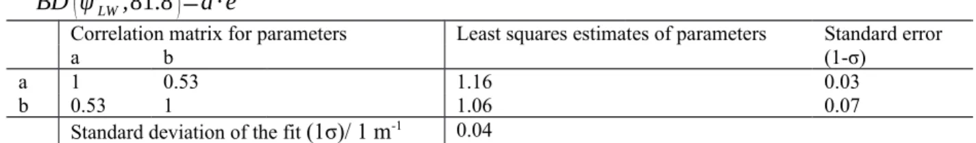
Table S10: Fit function to calculate rates of CO2 bubble dissolution (BD in 1 m^-1) as a function of the bubble distance from the seafloor (z in m) based on the initial bubble size distribution (ψLW) and water depth at which bubbles are released (81.8 m) during the leaky well simulations. The fit has been used to calculate the source rate of CO2 (S) of the leaky well scenarios (Eq. 4).

BD

(

^ψLW,81.8

)

^{=a ∙ e}^{−b ∙ z}

2

a b (1-σ)

a 1 0.53 1.16 0.03

b 0.53 1 1.06 0.07

Standard deviation of the fit (1σ)/ 1 m^-1 0.04

For data fitting, combined CO2 bubble dissolution rates have been used (details on the parameterization of the bubble dissolution model are given in Tab. 1).

29

30

31 32

(8)

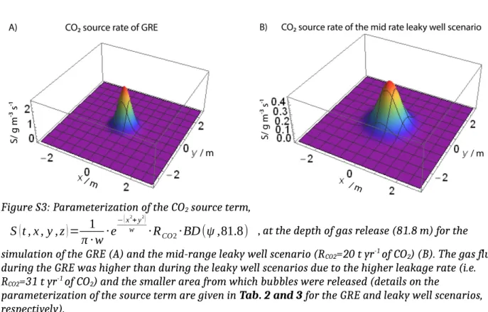
Figure S3: Parameterization of the CO2 source term,

S

(t , x , y , z)= 1

π ∙ w ∙ e

⁻

(x²+y²)

w

∙ R

_CO2

∙ BD

(ψ ,81.8) , at the depth of gas release (81.8 m) for the simulation of the GRE (A) and the mid-range leaky well scenario (RCO2=20 t yr^-1of CO2) (B). The gas flux during the GRE was higher than during the leaky well scenarios due to the higher leakage rate (i.e.

RCO2=31 t yr^-1of CO2) and the smaller area from which bubbles were released (details on the

parameterization of the source term are given in Tab. 2 and 3 for the GRE and leaky well scenarios, respectively).

34 35

(9)

2. Setup of the COMSOL model to simulate the GRE

Table S11: Setup of the plume dispersion model in COMSOL Multiphysics in order to simulate the GRE by coupling the k-ɛ turbulence model (spf) and transport of diluted species (tds) physics interfaces.

Coupled physics interfaces to simulate the GRE Physics Interface k-ɛ turbulence model (spf) with

Turbulent Mixing subnode

Transport of Dilutes Species (tds)

Model Inputs Fluid Properties: Seawater density and Dyn. Viscosity of seawater Turbulence Parameters: IT and LT

prescribed as Inlet Boundary Condition

Velocity field (u, from spf solution)

Diffusion Coefficient: DM=10^-9 m² s^-1 DT (from spf solution)

Source Rate: S

Initial Values u=0 C=0

Boundary Conditions Inlet: Velocity Condition (Normal Velocity: Fit to ADCP Data) Outlet: Pressure Condition (Normal

stress P=f0=0)

Wall: slip (no viscous stress at the

sides and top)

Wall: no-slip (Boundary Condition of

the Lander geometry and seafloor), Wall roughness length= kseq

Inflow through northern Boundary (B.):

C=0

Outflow through southern B.: n (-

D∇C)=0 (ignores diffusion) No Flux: at all other boundaries

Model Geometry Rectangle model domain of 50x20x20 m³ in x,y,z with a smaller rectangle of 2.2x0.7x2.2 m³ in x,y,z in its center (in accordance to the geometry of the Ocean Elevator).

Mesh (user-defined) Extra Fine: Free Tetrahedal (dxmin=0.075 m; dxmax=1.75 m)

Local Mesh Refinement along Lander Boundaries (dxmin=0.1075 m; dxmax=0.2 m) Boundary Layers along the no-slip BC at the seafloor

Model Simulations Rotation of Ocean Elevator: 40°, 70°

3 Spatial heterogeneity of DIC concentrations in the CNS 36

37

38

(10)

transect in the Tommeliten seepage area. The DIC heterogeneity of 16 µM was assumed to be also representative for the Sleipner area, due to similar physicochemical conditions of seawater and was thus, used as a geochemical threshold for leak detection.

39

Supplementary material for:Footprint and detectability of a well leaking CO