Cruise No. POS483
Palinuro Volcanic Complex, Tyrrhenian Sea 2015
Marion Jegen
EMPAL: Electromagnetic investigation of sedimented Massive Sulphide deposits on the Palinuro Volcanic Complex in the Tyrrhenian Sea.
28.3.2015 – 15.4.2015
Malaga – Dubrovnik
Table of Contents
1 SUMMARY ... 3
2 PARTICIPANTS ... 4
3 RESEARCH PROGRAM ... 4
4 NARRATIVE OF CRUISE ... 8
5 PRELIMINARY RESULTS ... 13
5.1 Electromagnetic Experiments ... 13
5.1.1 CSEM – Dipole-‐Dipole (Sputnik) ... 13
5.1.2 Self Potential ... 17
5.1.3 CSEM -‐ Loop (Octopussy) ... 19
5.2 CTD water column measurements ... 22
5.3 Geological Observation ... 24
5.3.1 Geology of the Palinuro Volcanic Complex: ... 24
5.3.2 Geology of the Western Sector: ... 25
5.3.3 Hydrothermal Deposits: ... 27
5.3.4 “Sputnik” Site Observations during POS483: ... 28
5.3.5 HyBIS Observations and Geological Interpretation: ... 29
5.3.7 Photogrammetric Mapping: ... 32
5.3 Passive Seismic Experiment ... 35
5.4 Summary ... 35
References: ... 37
6 SHIP’S METEOROLOGICAL STATION ... 39
7 STATION LIST P483 ... 39
7 DATA AND SAMPLE STORAGE AND AVAILABILITY ... 47
8 ACKNOWLEDGEMENTS ... 47
10 APPENDIX ... 48
1 Summary
Investigations of submarine massive sulfides (SMS) are, at present, strongly limited due to the technologies available. Conventional detection of SMS deposits relies on water column plume detection of seafloor hydrothermal venting and seafloor morphological observations. These methods are generally confined to known regions where SMS are currently forming and where these deposits have a surface expression. Within this cruise we aim to test existing and new electromagnetic instrumentation, which detects and characterizes SMS deposits based on their associated electrical conductivity anomaly. This technology will allow us to detect sedimented deposits and potentially much larger SMS deposits which have completed their formation cycle, but have no surface expression. We tested the technologies on partially sedimented SMS deposits on the Palinuro volcanic complex situated in the Marsili back-arc basin. This region has been mapped in detail, SMS deposits have been drilled and drill cores are available at Geomar such that electrical conductivity of the particular units may be determined. The geological background information thus allows us to calibrate and ground truth the electromagnetic measurements. The development of the technology we are testing is funded through the funded EU proposal ‘Blue Mining’ and scheduled to be used on the TAG SMS deposit on the Mid-Atlantic Ridge at 26°N in 2016 as an example for resource assessment technology.
Die Erkundung submariner Massivsulfide (SMS) ist durch die herkömmlich eingesetzten Technologien eingeschränkt. Sie stützt sich zur Zeit hauptsächlich auf das Aufspüren von Wassersäulenanomalien als Indikator der SMS Entstehung zugrundeliegenden hydrothermalen Aktivität und das Kartieren der Meeresbodenmorphologie mit anschließender Beprobung. Die Erkundung ist damit auf sich in Entstehung befindenden SMS und auf meeresbodenoberflächenahe Strukturen beschränkt. Auf dieser Ausfahrt wollen wir existierende und neu entwickelte elektromagnetische Instrumente, die SMS anhand ihrer Leitfähigkeitsanomalie identifizieren und auch in Tiefe abbilden, testen. Somit können auch SMS, welche den Entstehungszyklus beendet haben und somit wahrscheinlich sehr viel größer sind, gefunden und deren Ausmaße abgeschätzt werden. Der Test wurde auf Massivsulfiden des Palinuro Komplex im Marsili back-arc basin ausgeführt, da diese detailliert kartiert und erbohrt wurden und die am Geomar lagernden Bohrkerne dazu benutzt werden können, Leitfähigkeiten einzelner Fazien zu bestimmen. Somit kann die neu-artige elektromagnetische SMS Erkundung kalibriert und evaluiert werden. Die eingesetzten Geräte werden im Rahmen des EU Projekt ‘Blue Mining’ entwickelt und sollen 2016 auf TAG am mittelatlantischen Rücken, 26°N, als mögliche Technologie zur marinen Ressourcen- evaluierung eingesetzt werden.
2 Participants
Name Discipline Institution
Dr. Jegen, Marion Marine Geophysics / Chief Scientist GEOMAR
Dr. Petersen, Sven Marine Geology GEOMAR
Dr. Hölz, Sebastian Marine Geophysics GEOMAR
Prof. Hannington, Mark Marine Geology GEOMAR
Safipour, Roxana Geology CSM, USA
Grant, Hannah Geology GEOMAR
Broda, Benedikt Marine Geophysics INDUSTRY
Dr. Kwasnitchka, Tom Geology GEOMAR
Wollatz-Vogt, Martin Marine Technician GEOMAR
Matthiessen, Torge Marine Technician GEOMAR
GEOMAR: Helmholtz Institute of Ocean Research, Kiel, Germany CSM: Colorado School of Mines, Golden, USA
ALLSEAS: Marine Engineering Company, The Hague, Netherlands
3 Research Program
Fig. 3.1: Track chart of P483. Bathymetry from Smith and Sandwell (1997).
Seafloor massive sulfide deposits (SMS) are formed through hydrothermal circulation of seawater, a process by which metals are leached out of the host rock by hot fluids. The metal- rich fluid eventually exits at a seafloor vent field where the fluid cools and metals are
precipitated, ultimately forming a SMS deposit. Metals can also be precipitated in the subseafloor, often when a sediment cap is present and therefore minimal or no hydrothermal venting occurs. Venting may also occur either through high-temperature fluids at chimney structures such as black smokers or at lower temperatures in more diffuse vent fields.
Hydrothermal circulation is driven by heat and occurs mainly at marine plate boundaries such as mid-ocean ridges, volcanic arcs and back-arc basins where heat is supplied by increased magmatic activity. Along oceanic plate boundaries which stretch to a length of about 89 000 km (Bird, 2003), approximately 300 sites of present and past hydrothermal activity have been observed and 165 of these contain massive sulfide mineralization (Hannington et al., 2011). A statistical extrapolation of the occurrence of known vent fields and deposits suggest that about 500 to 5000 vent fields and associated sulfide deposits with a total accumulated volume of 600 millions tons containing 30 million tons of copper and zinc are present in the immediate vicinity of oceanic plate boundaries (Hannington et al., 2011). Due to the fact that SMS are compact structures close to the seafloor and some contain high-grade ores, the possibility of mining such massive sulfide deposits has gained much attention on a national and international level (Boschen et al., 2013). While much knowledge has been gained by studying SMS formed at active vent fields close to plate boundaries, there has been a shift in focus lately to take a broader view at extinct, that is, inactive SMS structures (eSMS), since they are believed to host 10 times more metals than the active systems and are thought to be larger than young active systems (Hannington et al., 2011). Although exploration for seafloor massive sulfides has moved to island arc systems in the past decade, there are still large gaps in our knowledge of the formation of deposits in this tectonic environment. Since exploration in island arcs is largely focussed on active hydrothermal fields being discovered through the use of chemical and physical-chemical tracers in the water column (de Ronde et al., 2007), we only know very few mature hydrothermal systems within the island arc environment. In general, volcanoes that do not show chemical signals of hydrothermal activity in the water column are not investigated any further; therefore, we only have limited information about the lateral and vertical extent and the volume of SMS deposits in arc systems. It is currently impossible to compare the size of island arc systems to those forming at mid-ocean ridges due to the lack of technologies to find them.
Addressing this issue is important for two reasons: 1) we do not know the metal potential of hydrothermal systems at island arcs. 2) we do not know if large sulfide deposits do actually form in island arc volcanoes or if frequent volcanic eruptions prohibit the formation of large deposits.
Mapping inactive SMS deposits requires the integration of new geophysical exploration technologies in SMS research. Currently the detection of SMS is mainly based on identifying signatures of active hydrothermal venting in the water column followed by, or in parallel with, seafloor morphological observations (i.e. bathymetry and video observations) and subsequent sampling. While these methods result in detailed studies of particular SMS deposits, it obviously gives only very indirect information about the volume of an SMS deposit and its vertical and lateral extent. These conventional approaches are however inappropriate for mapping extinct or blind deposits. Few blind or sedimented deposits are currently known and those that are have been found more or less accidentally, i.e. through heat flow data (Middle Valley Bent Hill deposit; Davis et al., 1987) or chance sampling (Palinuro volcanic complex; Minniti and Bonavia, 1984).
However SMS deposits are associated with rock property anomalies, and therefore they may be identified by geophysical methods and mapped below the seafloor even if they are covered by sediments and have an absence of active hydrothermal venting at the seafloor. In particular, massive sulfide deposits both on land and seafloor exhibit a strong electrical conductivity anomaly (i.e. Palacky, 1986 and Itturino et al., 2002), which is why electromagnetic methods are the tool of choice for ore exploration. Similar to land exploration, marine electromagnetic methods are expected to take a similar leading role for massive sulfide exploration on the ocean floor.
The detectability of SMS deposits by EM methods has been shown by Kowalczyk (2008) with a shallow penetration, ROV based EM tool on the Solwara site offshore Papua New Guinea. While the instrumentation was only been able to map the surface anomaly associated with surface SMS deposits, drilling results confirm that anomalous electrical conductivity are indeed associated with SMS. Cairns et al. (1996) report an electromagnetic pilot study to image the TAG Hydrothermal Field (26°N, Mid-Atlantic Ridge) SMS deposit. However, at the time electromagnetic instrumentation was in its infancy and 3D modelling capabilities were just in development and a 3D image of the sulfide deposit could not be derived.
Much progress in EM exploration have been made over the last 15 years, electromagnetic investigations are now routinely used for oil/gas exploration in industry and additionally for methane hydrate research. Thus the search for and 3D imaging of massive sulfides is technologically within reach.
Recent modelling studies at Geomar have shown that marine electromagnetic methods will indeed allow the identification of massive sulfide deposits and enable determination of their
thicknesses even under meters of sediments (Hölz et al, 2013, Swidinsky and Jegen, 2012, Jegen et al., 2011).
Figure 3.2 shows a map of the target areal. The drilled SMS deposit is annotated with A. We furthermore aimed to explore the Palinuro complex towards the East (target B in figure 3.2), where recent bathymetric surveys have revealed the existence of chimney structures (up to 15 m in height), which are thought to indicate the presence of hydrothermal circulation venting at surface. Another target area was to the North, where sidescan-sonar data revealed another area of chimneys that are up to 20m high and sit on presumably sulfide mounds up to 50 m in diameter (target C in figure 3.2).
The exploration technology is to be tested on the SMS deposit on the Palinuro volcanic complex (see figure 3.2). It is an ideal target, since it has been extensively researched and analyzed from a geological perspective providing us with extensive background data in the form of detailed bathymetric, parasound, magnetic and side scan sonar maps that were retrieved during an AUV survey in 2012 (Poseidon cruise P442, Petersen et al., 2013a and b). Furthermore, certain areas have been drilled which will give us structural information and the cores stored at Geomar may be used to derive rock properties such as electrical resistivity and magnetic susceptibility. This set up gives us the unique chance to calibrate our measurements and assess their quality as SMS
exploration tools. Since the Palinuro SMS is partially buried, it offers the possibility to verify SMS detection with electromagnetics under sediment cover. While all the geological background information forms the basis for our geophysical test, by the same token, the geophysical exploration will yield information about the size and volume of the known SMS deposit (and potentially other new SMS sites), and therefore will allow better understanding of the geological processes at work at Palinuro.
4 Narrative of Cruise
March 28th:
We left the port of Malaga in good weather in the afternoon, slightly delayed since we had to pick up some missing cables for the Posidonia navigation system. However, since the forecasted weather was good, we expected to arrive in our working area at the scheduled time of 8:00 AM on April 2nd. The day itself was used to unpack our boxes, set up the lab and instrumentation.
March 29th-April 1st:
We continued the preparation of experiments, the hook up and testing of the fibre optical winch for HyBis. During the evenings of the transit we scheduled a meeting at 19:00 in order to discuss organizational matters (who is responsible for which aspect of the cruise), subsequently we had informal scientific presentations and discussions on the geological and geophysical background and on the exact layout of the experiment.
April 2nd:
The day started positively, after some problems on previous days, we finally managed to get the Posidonia navigation system going. The calibration velocity profile was determined by a CTD microcat instrument attached to a cage, which was lowered to 600 m. The cage also contained the releasers and we were able to test their functioning at the same time. We then deployed the MORS transponder with an anchor in a sedimented area in the centre of our working area (39o 32,37' N, 14o 42,47' E). Calibration of the Posidonia system required two ship tracks in the shape of an 8 centred on the transponder. However, problems occurred when the seafloor Posidonia transponder did not release its anchor and resurface, even after a repeated release command was sent. This was problematic as this transponder was vital for the required precision of seafloor navigation in our later experiments. We developed plans to either dredge the transponder or try to recover it with HyBis. A watch was set up over night to check on the position of the
transponder hourly via ranging to ensure that it would not drift away if it resurfaced before the following workday started.
April 3rd:
The wind of fortune was changing again, as the Posidonia transponder resurfaced at 6:30 local time in the morning and could be recovered just in time before breakfast. We then started to deploy the OBSs and OBEMs, which were attached on the winch cable through the Posidonia transponder, which also serves as a releaser. The stations were released approx. 30m above the seafloor, such that the position of the systems is accurately known within a few m. During the remainder of the day we were able to deploy 6 OBSs and 7 OBEMs.
April 4th:
Within the morning hours, we deployed the remaining 3 OBEMs and prepared our
electromagnetic dipole source Sputnik for deployment. The source was in the water at around 15:00 UTC, however, a short circuit occurred while we lowered Sputnik to the seafloor, so the instrumentation had to be heaved back on the deck. Inspection showed that the short circuit occurred at the connector between the winch cable and Sputnik, which required a reconfiguration of the winch cable connector. The cause of the short circuit was probably a leak at the winch’s cable connector. A second deployment was tried at 22:00 UTC for an overnight transmission, however, it had to be aborted since the dipole arms did not unfold when Sputnik was placed on the surface. We attributed that fact to an incorrect buoyancy alignment on the lower end of the winch cable. Buoyancy aids were needed as the lower 10 m of the winch cable should be
positively buoyant to ensure that the winch cable is vertical to prevent the winch cable wrapping around the transmitter arms. This is achieved by attaching floatation eggs on the cable. The experiment was aborted and Sputnik safely recovered on deck at around 24:00 UTC.
April 5th and April 6th:
Sputnik went back in the water with one additional flotation egg after lunch and was able to transmit until about 18:40 UTC, when there were repeated problems with unfolding the arms, such that we needed to recover the instrument again. Shortly after the problems occurred, one of the floating eggs surfaced, which led us to believe that the arms did not unfold since the
buoyancy was again unbalanced. The floating egg could be recovered, but was damaged. We suspected that due to the fact that Sputnik had to be deployed over the A-frame, where the heave
is highest (sea was relatively rough with 3-4 m waves) and due to the flexibility of the 11 mm cable, the winch cable might wrap around the floating egg, causing it to detach.
Luckily, we had spare floatation eggs to add to the cable and redeploy Sputnik at 23:00 UTC.
During the night we were able to raise the amount of transmission sites to 27 until 10:30 UTC on April 6th, when Sputnik failed again. Upon recovery, we noticed that the winch cable had been wrapped around one of the floating eggs. Since the flotation egg could not be detached from the cable, a risky recovery had to be initiated. Sputnik was attached via Evergrip onto an auxiliary winch on the A-frame, and the mangled cable was cut off. We then decided to delay further Sputnik transmissions to calmer seas, when sea heave would be reduced. For the remainder of the day, we prepared HyBis, performed deck tests with HyBis and undertook a short water test in the evening.
April 7th:
HyBis went in the water at around 7:10 UTC to start the first visual dive. For the
photogrammetric survey a Sony CX-560-VE camcorder with a 0.7x wide angle converter installed in a 110mm diameter Develogic domeport housing was used. During the dive HyBis was kept at a height of approx. 3 to 5 m above ground. The first dive concentrated on the northeastern section of Palinuro, where during the AUV bathymetric mapping chimney-like structures were identified in the eastern part. However, visual inspection indicated that the
chimneys were not of hydrothermal origin as expected. This was a slightly worrying observation, since chimney structures are attributed to be one of the most reliable indicators of hydrothermal circulation. In particular, the number of chimneys visible in bathymetric maps are used to project the resource of metals in SMS deposits. The remainder of the dive was used to investigate the northwestern area of the section. Visual inspection confirmed hydrothermal activity through the observation of sediments with dark coloring and white striations. HyBis was subsequently recovered and back on deck at 14:30 UTC.
Since relatively high waves made the deployment of Sputnik with its unfolding arms over the A- frame impossible, we thought it a good opportunity to test a new technology called Self Potential (SP). The test was not part of the original cruise plan, however Russian exploration cruises previously reported good success with this methodology. SP senses the electrochemical potential created through fluid flow or contact of SMS deposits with the surrounding host. Since the measurement are taken while hovering a few meters above the seafloor, the experiment could be more easily carried out in the prevailing weather. To construct an SP sensor, OBEM 7 was
recovered, and its data logger and battery pack together with an additional data logger were installed on the Sputnik frame. Sputnik’s dipole arms were refastened to the frame to form 3 orthogonal dipoles so that the direction and amplitude of the SP signal may be measured.
April 8th:
HyBis was put into the water again for its second visual dive, this time investigating the southern, central and northwestern section of Palinuro. At the southern cliff, layering of lava- flows and volcaniclastics were identified. On the southwestern section, sediments with dark coloring and white striations were observed. The path over the central region led over one of the OBS systems. At 12:15 UTC HyBis was recovered and back on deck. Two and a half hours later, the Sputnik frame with the Self Potential configuration was lowered to the seafloor and data acquisition was continued through the night until the 9th of April.
April 9th:
After breakfast, at 6:00 UTC, the SP instrument was brought on deck so that the data could be checked. To free up time towards the end of the cruise when the weather was expected to get better and a redeployment of Sputnik would be possible again, we decided to bring up the OBSs earlier as scheduled. The 6 OBSs were recovered until 9:00 UTC. During the OBS recovery, the bow thruster of Poseidon broke with a big bang. A ball bearing broke, probably due to a water leakage into the thruster. For future experiments however, it meant that a precise manoevering of the vessel would be very difficult to achieve.
A quick sighting of SP data gave evidence of SP anomalies so we decided to continue with the SP measurements. Accordingly, the SP instrumentation was deployed again at 11:15 UTC and ran until 22:00 UTC. Due to the vessel’s problem with precise navigation we decided to perform a random path pattern covering as much as possible of the area of interest.
While the SP instrumentation was in the water, we prepared the virgin deployment of the coil system.
April 10th:
The morning started with a recovery of the SP instrumentation and Sputnik was reassembled in its original configuration of a dipole transmitter. We also redeployed the previously recovered OBEM station, this time free falling to save on time. Sputnik went into the water again at 13:15 UTC. To avoid potential mangling of the wire on the floating eggs, we decided to only use a single floating egg at the connector between the winch cable and Sputnik. However, it proved to
be insufficient, since Sputnik’s arms did not unfold when placed on the seafloor, which we attributed to the fact that most likely the winch cable was wrapped around the transmitter arms before they unfolded. Subsequently we brought Sputnik up to the water surface and attached another floating egg higher on the cable. Sputnik then performed sufficiently well and we managed to finish the planned transmission profile.
April 11th:
The coils system Octopussy went at 10:00 UTC in the water. The deployment procedure went astonishingly smoothly given the size and length of the system. Since all electronic devices were functioning when tested in the water column, we decided to bring the system down onto the seafloor and acquire data along one long profile. The system was recovered at 16:00 UTC.
April 12th:
Our last day in the working area. Recovery of the 10 OBEM stations was achieved in record time between 06:00 to 9:30 UTC. A motivation for the speedy recovery was the prospect of being able to reach the Stromboli volcano before sunset and using the stunning scenery as a backdrop of our celebratory end of cruise Stromboli party, which was attended by the entire scientific party and a large proportion of the crew.
April 13th:
We left Stromboli in the early morning hours to pass through the Straits of Messina at around 06:00 UTC. The remainder of the day was used to take a break and relax in the sunshine. After all it was Sunday, all the envisioned work was completed, and the party has been good.
April 14th:
Instrumentation was disassembled, laboratories packed and cleaned. By 18:00 a neat stack of boxes and instrumentations was assembled on the back deck ready for offloading on the next day.
April 15th:
We arrived in Dubrovnik by 9:00 local time. Unloading of our gear from the ship and loading the trucks was completed by about 14:00 local time.
5 Preliminary Results
5.1 Electromagnetic Experiments (M. Jegen and S. Hölz)
Within the scope of this project we are testing two different active electromagnetic methods based on a dipole-dipole configuration and a magnetic coincident loop system as well as a passive method called Self Potential (SP). This method aims to record static electrical potentials caused by geochemical processes occurring on the boundary of SMS deposits.
5.1.1 CSEM – Dipole-Dipole (Sputnik)
This electromagnetic experiment consists of a time domain controlled source electromagnetic approach using dipole receivers and the dipole transmitter (see figure 5.1.1).
The electromagnetic dipole receivers are deployed on the seafloor on a winch cable to ensure exact positioning. The instruments record orthogonal electric field variations at a frequency of 10 kHz when in CSEM mode and three component magnetic field and 2 component electric field variations at a frequency of maximal 10 Hz when in magnetotelluric (MT) modus. The
acquisition modus can be changed actively by an acoustic signal or predefined through a timetable.
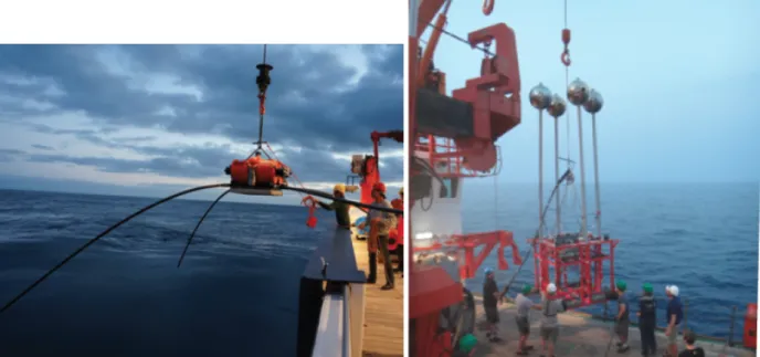
When in CSEM modus the receivers record the Earth’s response to an active dipole source signal generated by the Sputnik transmitter. The transmitter consists of two orthogonal 14 m electrical dipole arms, which fold up when the system is hanging on its own weight on the cable and unfold when system is placed on the seafloor. The transmitter current is supplied and regulated through DCDC converters, buffer batteries and a microprocessor controller. These units are housed in titanium cylinders, which are attached to the central frame, which also carries an altimeter, light and camera. A fast modem connection between a deck unit and transmitter frame is established through the winch cable for online control of transmitter activity and data transfer.
Knowledge about the exact positioning of the transmitter during a transmission cycle is achieved through the attachment of a Posidonia transponder onto the frame and through our own short baseline navigation system. This consists of an acoustic receiver array on the frame which communicates/ranges the releasers on all the receivers both before, and after, each transmission.
The diffusion time of the electromagnetic signal from transmitter to receiver as well as the amplitude of the received signal depend on the resistivity of the seafloor. Vertical resolution is achieved through measuring the response at different distances between transmitter and receivers as well as over recording the signal over a broad time scale. Additional resolution may be
derived from measuring the response to different polarization modes. For this reason both the transmitter as well as the receivers transmit and receive the electric fields in orthogonal directions.
Figure 5.1.1: The Time Domain Electric Dipole-Dipole system consisting of OBEM receivers (left) and the Sputnik transmitter (right).
Ten OBEMs were deployed on the 3rd and 4th of April at the following coordinates:
Station ID Latitude Longitude Date Time OBEM 1 39° 32.542 14° 42.347 3.4.2015 12:11 OBEM 2 39° 32.575 14° 42.478 3.4.2015 13:10 OBEM3 39° 32.578 14° 42.652 3.4.2015 14:03 OBEM 4 39° 32.417 14° 42.628 3.4.2015 15:05 OBEM 5 39° 32.281 14° 42.605 3.4.2015 15:55 OBEM 6 39° 32.260 14° 42.449 3.4.2015 16:50 OBEM 7 39° 32.276 14° 42.330 3.4.2015 17:33 OBEM 8 39° 32.38 14° 42.330 4.4.2015 07:24 OBEM 9 39° 32.379 14° 42.400 4.4.2015 08:33 OBEM 10 39° 32.411 14° 42.452 4.4.2015 10:46
The receivers were released from the winch cable at approximately 30 m above the seafloor.
OBEM 7 was recovered on 7.4.2015 and used as a data logger for the SP experiment. It was redeployed in the morning of the 10.4.2015 at 39o32.25' N, 14o42.40' E as OBEM11. All OBEM stations were recovered in the morning of 12.4.2015.
Sputnik was first deployed at around 13:00 UTC on 4.4.20215 over the A-frame on an 11 mm cable. However, the transmissions were repeatedly interrupted by either short circuits in the connection cables or problems with the floats attached on the cable above the source, which are needed to keep the cable upright to avoid that the cable wraps around the dipole arms.
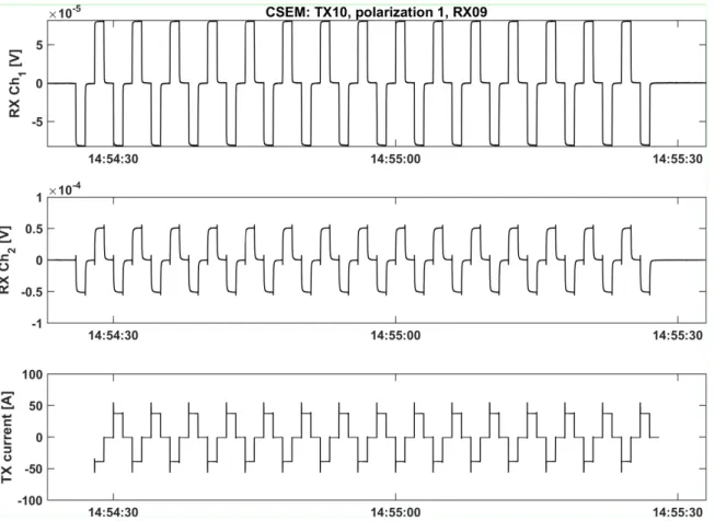
Altogether, transmissions at 22 stations were performed in the period until the early morning of 6.4.2015. Figure 5.1.2 shows the layout of the experiment and Figure 5.1.3 the transmitted wave form at transmission site 10 and a sample of the received signal at OBEM 9. Due to the high heave of the vessel’s back due to about 3 to 4 m high waves, further transmissions were delayed to 10.4.2015, when the sea was calmer. Unfortunately when we recovered the OBEM stations only receivers OBEM 4, OBEM 9 and OBEM 7 were fully functional for the entire time of deployment. The other receivers only recorded part of the signal due to a previously not fully unexplained failure in the data logging routine. All SD cards, which store the data on the logger, have been tested prior to the experiment, alas for shorter periods than the duration for the
experiment. A possible failure mechanism we are investigating at the moment is that the writing speed for the suite of SD cards used has increased causing a synchronization problem with the data acquisition software for large data packets as acquired during deployment.
Nevertheless the data acquired on the receivers is of good quality and will allow us to derive resistivity values of the subsurface up to depths of 10s of meters.
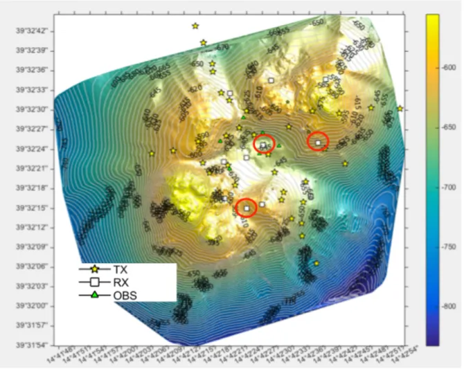
Figure 5.1.2: Layout of the CSEM Dipole-Dipole experiment. Yellow stars mark the position of transmission sites and white squares the location of the receivers. Fully functioning receivers are encircled in red. Also shown are the locations of the OBS as green triangles.
Figure 5.1.3: Sample data set for one transmitter polarization acquired during the experiment.
The upper two panels show the response measured at station RX09 for a current transmitted at site 10 at a distance of approx. 150m from the receiver (lower panel).
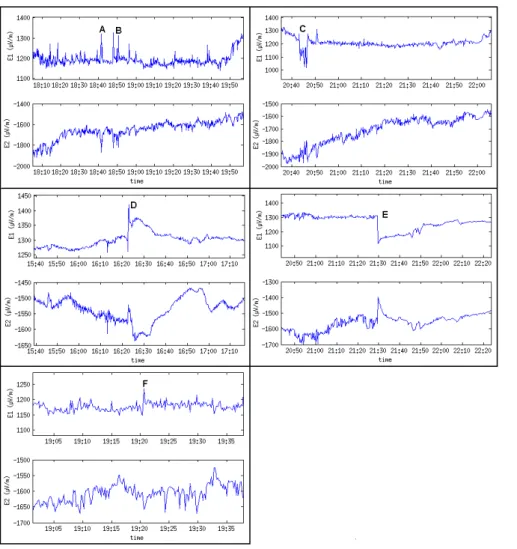
5.1.2 Self Potential
Figure 5.1.4: Left: SP experiment track for dive 1 of Sputnik (white crosses) and dive 2 (black crosses). The second track was chosen to consist of random drifting, since the bow thruster malfunction made it very difficult for the ship to maintain position. Right: Location of SP anomalies identified in a preliminary data analysis.
Self Potentials are naturally occurring electric voltages due to charge accumulation, which may arise from three different processes: 1. fluid flow in porous media, 2. thermoelectric potentials due to temperature gradients and 3. diffusion potentials which occur across boundaries between different geochemical compositions. The latter are usually of the greater significance in
geophysical exploration on land. Marine SP anomalies on SMS deposits have been reported at various conferences, however, up to now no peer-reviewed publication exists. Since the Sputnik transmission had to be postponed to a later date with calmer seas, we decided to equip the Sputnik frame with receiver electrodes and data loggers and try out SP measurements. Since no spare data logger was available, one of the OBEM stations (OBEM7) was recovered and dismantled. The left panel of figure 5.1.4 shows the tracks along which SP measurements were acquired with a 10 Hz sampling rate at a distance of approximately 5 to 10 m above the seafloor.
Figure 5.1.5 shows excerpts of the acquired time series in which a clear spike above the telluric noise level is observed on both electric field components and which probably constitutes an SP signal. The locations of the preliminary data processed are shown in the right panel of figure 5.1.4 . The occurrence of the SP anomaly at location A, B and D as well as F coincide with known SMS locations. However, to correlate the signal with geological observations, further data analysis is required and has to be developed. The development of modeling and processing algorithm is part of the PhD project of Roxana Safipour and will be carried out in collaboration with her supervisor, Prof. A. Swidinsky at the Colorado School of Mines in Golden, Colorado.
Figure 5.1.5: Plot of the SP anomalies shown in figure 5.1.4. As characteristic for the anomaly, we defined a visible change in both components of the horizontal electric field above the
naturally occurring telluric current variations in time observed during at constant sensor height above seafloor.
5.1.3 CSEM - Loop (Octopussy)
While the 3D dipole-dipole tomographic system has greater resolution power due to the fact that multiple receivers are deployed and measurements are made at different offsets, the data processing for this system is sufficiently involved that data cannot be processed on-ship.
Regional exploration however would benefit greatly from a system that could give real time information, at least on a qualitative scale, on the presence of subseafloor SMS deposits. That condition can be best met by a coil system. The system uses a coil as a transmitter. When a DC current is suddenly switched off, a smoke ring of current is induced at the seafloor, which will propagate upwards and sideways. The propagation speed and the dampening of the amplitude of the current can be measured using the same coil. Due to the relative simple and constant geometric set up of the system, and since the current patterns produced by the system are relatively simple and sensitive to seafloor resistivity immediately below the system, the coil data can immediately be interpreted qualitatively without undergoing any data time consuming
modeling. We are therefore currently constructing and testing such a time domain coincident coil system.
The prototype coil used during this cruise consists of a 4m x 4m GFK frame mantling the coil cable. On the coil, two tiltmeters monitoring the orientation of the coil are mounted. Pressure vessels housing the electronics, i.e. transmitter driving circuitry, communication ports as well as an altimeter are attached to a second GFK frame approximately 14 m above the coil. This distance between coil and frame is required to avoid any bias in the data due to induction in the pressure vessels. The transmission of electromagnetic energy is controlled from the ship and transmission current, altimeter and tiltmeter readings are displayed online. Up to now, the receiver data is recorded autonomously on a data logger, however, we plan to interface the logger online from the ship in the future such that conductivity anomalies may be detected live and offer the possibility to adapt the survey during measurements.
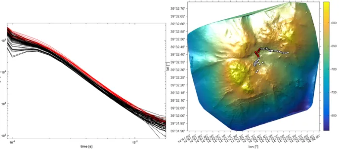
A first test of the system in the water was achieved on 11.4.2015. Figure 5.1.6 shows photos of the Octopussy system during deployment. Since the prototype was electronically and mechanically stable in the water column, we lowered it to the seafloor and performed a transect across Palinuro shown in figure 5.1.7. A first preliminary data sighting suggests, that there is a region surrounding the known vent site where the processed transients indicate an increased conductivity, which may be associated with the presence of hot hydrothermal fluid of massive sulfides. The anomalous region extends well beyond the region identified by surface observation of vent sites. It should be noted however, that the coincident loop data set collected is the first of the world of this kind.
Figure 5.1.6: Deployment of Octopussy. Left panel shows the deployment of the 4x4 m transmitter/receiver coil, right panel the GFK frame on which the instrument’s electronic devices were installed.
Figure 5.1.7: Left panel: Summary of all preliminary processed transients recorded along profile. Black colour denotes transients with average seafloor conductivity and red transients with elevated conductivities. Right panel: Circles show the location of loop measurements on Palinuro. The start of the profile is in the southwest, the end of profile in the northeast.
Locations where preliminary processed data suggests increased conductivities are marked in red. They coincide with the location of the known vent, but indicate that the hydrothermal area seems larger than indicated by surface observations.
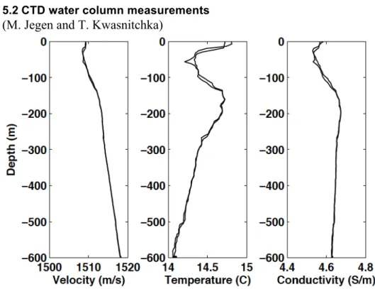
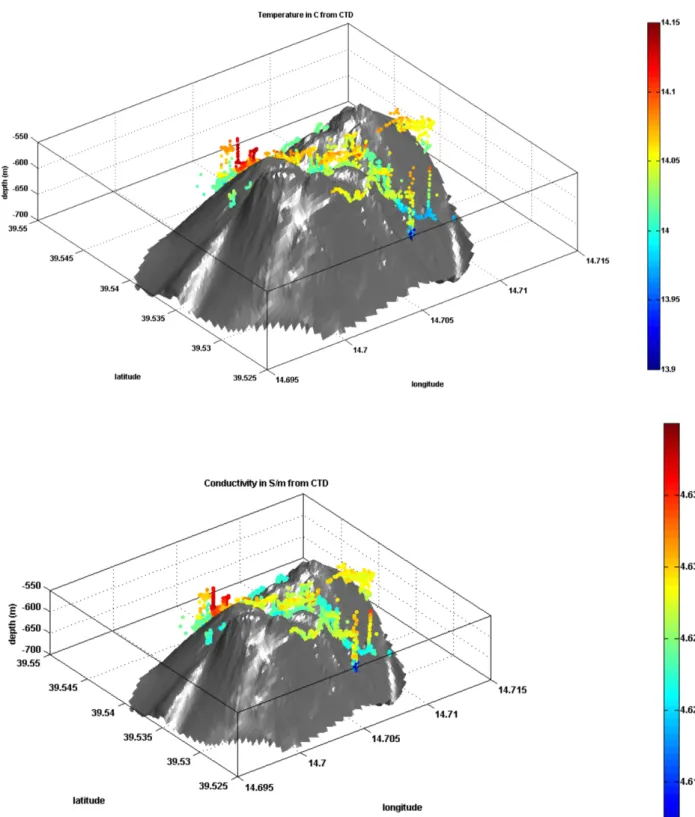
5.2 CTD water column measurements (M. Jegen and T. Kwasnitchka)
Figure 5.2.1: Velocity, temperature and conductivity profile acquired with a microcat CTD sensor from Seabird on April 2nd.
During most of the dives, an autonomous microcat CTD sensor from Seabird was attached to the frames. Figure 5.2.1 shows a velocity, temperature and conductivity profile acquired on the 2nd of April during the releaser test. The velocity profile was used in the calibration of the Posidonia navigation system. Evident is the relative high electrical conductivity of the water (>4 S/m as opposed to approx. 3 S/m in open ocean) due to the increased salinity in Mediterranean waters and relatively warm bottom temperatures of 14 C.
Figure 5.2.2 shows the observed changes in temperature and conductivity during all dives. There seemed to be a spatial scatter in the temperature and conductivity data. However, it is unlikely that variations are related to geological features. The scatter may be explained by the fact that the time of the day of the data acquisition and prevailing time are different for different dives. The corresponding changes in electrical conductivity at these depths are too small to be needed to take into consideration for electromagnetic modeling. However, the larger scale changes
towards the sea surface are sufficiently large to have an influence on the data interpretation and will be considered according to the measurement values.
Figure 5.2.2: Measurements of bottom water temperatures (< 550 m) (upper panel) and conductivities (lower panel) plotted for all dives. Measurements were taken at different times during the day and during tidal cycles, which may attribute to the variations in the data.
5.3 Geological Observation
(S. Petersen, M. Hannington and T. Kwasnitchka) 5.3.1 Geology of the Palinuro Volcanic Complex:
The Palinuro volcanic complex is part of the Aeolian Volcanic arc in the Tyrrhenian Sea, a semi- closed basin in the Western Mediterranean that opened as a result of roll back of the Ionian slab (Morelli, 1975; Kastens and Mascle, 1990, Carminati et al., 1998). The volcanic complex is located ~30 km NE of Marsili seamount in the adjoining Marsili back-arc basin. The oldest dated volcanic rocks from Palinuro have an age of 0.8 m.y. (Savelli, 2002). Fresh lavas from the top of the shallowest major cone have a K-Ar age of ~350,000 years (Colantoni et al., 1981). Calc- alkaline basalt and basaltic andesite samples recovered from Palinuro have a clear affinity to volcanic rocks of the Aeolian islands, although it remains unclear whether Palinuro is structurally part of the Aeolian Arc (Colantoni et al., 1981; Passaro et al., 2010).
The volcanic complex comprises at least 8 separate cone-like features that coalesce at their base, forming a single elongated edifice extending for about 55 km from east to west (Monecke et al., 2009; Passaro et al., 2010; Fig. 1). The basal width of the complex is ~25 km. It rises from the abyssal plain (3,400 m depth) in the Marsili Basin to a minimum depths of ~80 m in its central part. The southern flank of Palinuro, facing the Marsili back-arc basin, is characterized by steep scarps; the northern margin is onlapped by sediments of the nearby shelf. The volcanic centers are thought to be aligned along a major lithospheric fault system that defines the northern limit of the Calabrian domain on mainland Italy (Ghisetti and Vezzani, 1981; Tamburelli et al., 2000;
Rosenbaum and Lister, 2004).
The morphology of the complex is more complicated than the much younger volcanic cones of the Aeolian arc, such as Stromboli. It can be divided into western, central and eastern sectors that are strongly structurally controlled (Fabbri et al., 1973; Marani et al., 1999; Monecke et al., 2009; Passaro et al., 2010; Ligi et al., 2014). The main volcanic cones are dissected by
numerous WNW-ESE, WSW-ENE and ~N-S-trending faults that are thought to reflect a regional stress field. The major cones are elongated in a WNW-ESE direction and are located at
intersections of WNW-ESE and WSW-ENE oriented fault systems; volcanic ridges and collapsed calderas are more locally controlled by a ~N-S striking fault system. Hydrothermal activity and mineralization at two locations in the western sector are found where local volcano- tectonic features interact with regional tectonic structures (Ligi et al., 2014).
5.3.2 Geology of the Western Sector:
The western sector of the Palinuro complex comprises a large, ~8 km-wide depression bounded by a steep scarp in the south, an arcuate arrangement of volcanic edifices (most likely
structurally controlled) in the north and west, and a WNW-ESE trending volcanic ridge to the northeast (NE Ridge) that reaches a minimum water depth of 500 m (Figure 5.3.1). The extent of erosion of the western part of the volcanic complex suggests that it is old. The morphology is partly a result of gravitational collapse of a pre-existing edifice and more recent movement of a complex fault network.
The “NE Ridge” and adjacent depression was the focus of study during POS483. This part of the volcano includes 3 local highs at its summit, cut by a WSW-ENE and a N-S fault that form a small central depression. These features are thought to be the eroded remnants of a larger cone that was developed at the northeast margin of the western sector. No recent volcanic activity has been documented, although the main WSW-ENE fault and several smaller structures appear to have been occupied by dikes. The largest dike-like feature occupies the western part of the WSW-ENE fault and is clearly seen in the bathymetry on the western flank of the older intact part of the cone. Almost all surfaces of the volcanic complex are covered by at least a few centimeters to several meters of hemipelagic mud and volcaniclastic deposits. The underlying volcanic rocks in the small central depression and on the northern ridge have been affected by widespread hydrothermal alteration, indicated by a large area of demagnetization that was targeted during POS483.
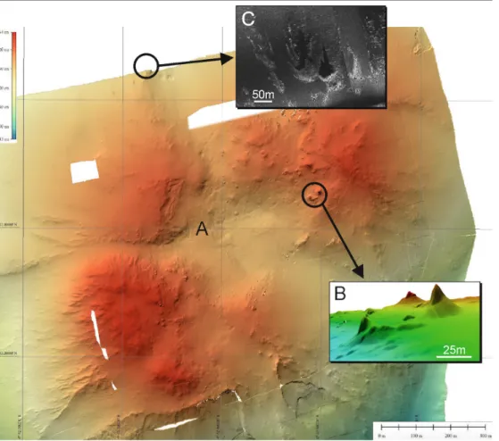
Figure 5.3.1: Bathymetry of the Palinuro volcanic complex from Petersen et al. (2014). A. High- resolution bathymetric map showing the location of the working area in the western sector. The rectangle (2B) indicates the area where the surveys were performed at the summit of the “NE Ridge”. B. High-resolution (10-m grid) bathymetry of the study area and the location of the drilled subseafloor barite and sulfide deposit. C. Interpreted geological section of the eroded remnants of a larger cone erupted on the NE flank of West Palinuro Seamount (see Figure 5.3.3 for details).
5.3.3 Hydrothermal Deposits:
Seafloor sulfides were first discovered by dredge sampling and gravity coring in the early 1980s, approximately 5 km west of the current study area (Minniti and Bonavia, 1984). Massive
sulfides were then discovered in the smaller depression of the “NE Ridge” during RV Sonne Cruise S041 in 1986 (HYMAS I). This has since been visited during POS340 in 2006, POS412 in 2011 and POS442 in 2012, and Meteor cruise M73/2 in 2007 and M86/4 in 2012 (Petersen et al., 2008, Monecke et al., 2009; Thiel et al., 2012, Petersen et al., 2014). Italian researchers visited the site during the RV Urania Mar98 cruise in 1998.
No black smoker activity has been found, but the central depression of the “NE Ridge” is characterized by widespread staining of the fine-grained sediments and local shimmering water indicative of low-temperature hydrothermal activity and diffuse venting through the sediment cover (Petersen et al., 2008). However, only a weak plume signal was found during dedicated plume surveys (Lupton et al., 2011). In 2006, small tubeworm colonies (Vestimentifera) were found on a sedimented slope at the northwest corner of the central depression, near the WSW- ENE fault (Thiel et al., 2012). This was the first discovery of vent-associated tubeworms outside the Pacific. The local fine-grained sediment contains minor disseminated sulfides, Mn–Fe oxides and clay minerals and is characterized by patchy discolorations, delicate chimney-like iron oxide structures, and bacterial mats (Monecke et al., 2009). This, and several other areas where there is evidence of hydrothermal activity (Figure 5.3.2) have high backscatter, contrasting with other parts of the summit area covered by fine-grained sediments. The high backscatter does not correlate with seafloor roughness but is associated with Fe-Mn oxyhydroxide crusts.
In 2007, the area of hydrothermal activity at the northwest corner of the central depression was drilled using BGS Rockdrill 1 (Meteor cruise M73/2). The drilled cores included up to 5 m of massive sulfides and barite from a few centimeters up to several meters below the sediments (Petersen et al., 2014). Eleven holes were drilled with a total core recovery of 13.5 m, including 12 m of semi- to massive barite and sulfides and 1.5 m of volcaniclastic rocks from an area of 50 m × 35 m. However, the lateral extent of the mineralization was not tested, and all drill holes ended in massive sulfide. The sulfides are thought to be more widespread, beneath a thickening sediment cover away from the center of the deposit. During POS442, buried and apparently inactive hydrothermal deposits were also discovered along the top of the northern volcanic ridge by AUV photography. Chimney-like features were also found by high-resolution bathymetry
and sidescan sonar surveys; however, several of these have been found to be volcanic pinnacles covered by coral (see below).
5.3.4 “Sputnik” Site Observations during POS483:
Upon landing, the camera of the Sputnik system showed that all but a few of the CSEM sites were heavily sedimented with typical marine clay and, in some cases, extensive burrowing (Figure 5.3.2). Only two stations landed on or near obvious outcrop. The sediment at TX08 and TX21 on the northern high was notably mottled, typical of the discoloured sediment found near the drill site. Volcaniclastic material or gravel (from slides) was observed at TX14, on the southern flank of the complex and adjacent to the headwall of the southern scarps, and at TX06 on the northern flank of the complex. TX20 landed near several irregular black outcrops
resembling Mn-coated coral, similar to that seen near the drill site. TX13 also landed on outcrop near the eastern dike-like feature on the flank of the volcanic complex.
Figure 5.3.2: Sputnik stations geological observations during landing.
5.3.5 HyBIS Observations and Geological Interpretation:
Figure 5.3.3 shows the interpreted geology of the summit area of the “NE Ridge” based on high- resolution bathymetric data and new HyBIS observations. The mapping and video observations confirm that the volcanic geomorphology is that of a heavily dissected and partly eroded cone.
The original cone was apparently formed by pyroclastic eruptions (mainly submarine but also possibly subaerial) and, at times, more effusive lava flows. At least 3 volcaniclastic units (V2, V4, V5), each 10-20 m thick, and 2 lava flows (L1 and L3) are suggested by the terraced morphology of the eroded summit. Blocky lavas were clearly visible at the edge of one terrace (L2) during station 137. All other outcrops appeared to be mainly cemented volcaniclastic material. Bedding planes between volcaniclastic units and lava flows appear to have a shallow dip.
The prominent dike-like feature exposed on the west flank of the cone can be projected under the volcaniclastic deposits of the summit area in the WSW-ENE fault. It may have been the feeder dike that is now buried by its eruptive products. The fault (and dike) dip steeply to the south, and this partly controls the morphology of the central depression. Other dike-like features may be present on the flanks of the volcano, but these are smaller and lack the clear magnetic signature of the main “feeder” dike. Prominent features on the northern high (so-called
“pinnacles”) appear to be composed mainly of blocky coherent volcanic material that may be eroded remnants of these smaller dikes. They are now partly covered by coral formations.
Extensive mass wasting has occurred on the south flank of the complex. The headwalls of the main erosional scarps may coincide with exposures of the two lava flows shown in Figure 5.3.2.
These are presumably more competent units that would have produced large slumps when they failed. A distinctive field of blocky debris can be seen on the SE slope of the complex, which may be traced back to the lowermost lava flow (L1) in the central depression. Although bedded volcaniclastic material is seen at the edges of the main scarps, generally this material is too fine- grained to have produced the larger blocks seen on the SE slope.
The main area of mineralization that was drilled in 2007 is located at the edge of the central depression near the proposed “feeder” dike. This mineralization and two other sites of inferred hydrothermal activity occur in at least two volcaniclastic units (V2 and V4) that are separated by coherent lava flows. Most likely, the localization of hydrothermal activity is controlled by the permeability contrasts between the volcaniclastic units and the coherent lavas. The currently
exposed mineralization is characterized by Fe and Mn crusts or cemented volcaniclastics, white patches and streaks (bacteria and/or barite) and distinctive dark staining and mottled textures in the sediments. These areas have a distinctive hummocky appearance (low mound like features with dark sediment between the hummocks (Fig. 4), which is very different from the background sediments. This hummocky surface may be produced by sediment-covered hydrothermal
deposits. The patchy or mottled texture is due to burrowing organisms that have excavated variably coloured reduced and oxidized subseafloor sediments.
Figure 5.3.3: Interpreted geology of the NE Ridge of West Palinuro Seamount. The map view shows the outlines of the lower contacts of volcanic units in the summit area. The present volcanic geomorphology is erosional, dominated by 3 erosional remnants of a much larger volcanic cone. The inferred location of a feeder dike is indicated (bold dashed line) extending from the west flank of the volcano, where it has an obvious bathymetric (and magnetic) expression, under the exposed volcanic units. The locations of the known mineralization are indicated by the stars. Section A-A’ shows the interpreted stratigraphy, which comprises south- dipping volcaniclastic units on the south side of the complex, and flat-lying or north-dipping units in the north. The proposed feeder dike is the most likely source of the volcaniclastics.
Figure 5.3.4: Photomosaic of hummocky terrain next to areas with dark coloring and white striations (on right side of the image) interpreted to be hydrothermal in origin. Photomosaic is based on AUV-ABYSS data collected during POS442 in 2012. Location in the vicinity of 39o32.52 N and 14o42.48 E.
5.3.6 Summary:
The NE Ridge of the western sector of Palinuro Seamount originated as a cone-shaped volcano that has been dissected along a WSW-ENE buried dike and secondary N-S faults. The original volcanic edifice was typical of the other cones of the western, central, and eastern sectors and likely formed at the margin of the much larger and older cone to the west (inferred caldera complex of Ligi et al., 2015). There are no convincing volcanic constructional features responsible for the present volcanic geomorphology of the NE Ridge. The original conical edifice is still visible in the regional bathymetry, but only the erosional remnants remain of the summit. Shallower water depths in the past may be indicated by the extensive coral formations, and the tectonic uplift of the volcano may have been caused by the nearby subducting Ionian plate or compression along the Adriatic foreland. Similar uplift likely caused the erosion of flat-
hummocks
hydrothermal
topped cones in the central sector. The NE Ridge has since been subject to extensive post-uplift deformation, subsidence, and collapse. Evidence of more recent volcanism was not found;
however, ongoing low-temperature hydrothermal activity must reflect a recent reactivation of the buried feeder dike.
Additional Figures in Appendix A:
Hybis_tracks_all. Edited Posidonia positions for HyBIS stations 135 and 137.
Hybis_1A. Annotated segments of dive track for HyBIS station 135 (part A) Hybis_1B. Annotated segments of dive track for HyBIS station 135 (part B)
Hybis_2_A_B. Annotated segments of dive track for HyBIS station 137 (part A and B) Hybis_2_C_D. Annotated segments of dive track for HyBIS station 137 (part C and D)
5.3.7 Photogrammetric Mapping:
Building on the AUV multibeam map as a reference, we chose to attempt the photogrammetric survey and reconstruction of assumed hydrothermal vents and key outcrops on the seafloor hinting to any other hydrothermal activity, following the methodology outlined in Kwasnitschka et al., 2013.
The HyBIS was outfitted with a special lower skid to house a battery powered, internally recording 1200KHz RDI Sentinel ADCP with bottom tracking capabilities which was used to measure vehicle motion relative to the water column and the seafloor. The ADCP was set to one second ping intervals. Additionally, the Posidonia USBL transponder mounted on HyBIS provided a USBL position fix every six seconds owing to its untethered responder mode in which there is no wire connection among pinger and antenna. As an experimental improvement to the aforementioned workflow, it was originally planned to connect an SBG Ekinox inertial navigation system both to the ADCP and to Posidonia using a serial port of HyBIS, yet this did not succeed due to hardware and software issues during installation on board. A Sony CX-560- VE camcorder with a 0.7x wide angle converter powered by a 5000MAh NiMH accumulator was installed in a 110mm diameter Develogic domeport housing and mounted at a 30°
downward angle on the skid, thus forming a self contained camera system. The internal
recording media was set to maximum quality and delivered 64GB of data on each deployment, covering 6h15min to which duration the dive times were scheduled. Due to some initial setup misunderstandings, the azimuthal viewing direction of the survey camera was 90°
counterclockwise offset from the front HyBIS viewing direction, so two of its LED lamps were
reconfigured to illuminate the survey camera’s field of view. One of the HyBIS low light online cameras was mounted parallel to the survey camera to monitor its field of view.
The system worked reliably during dives on station 136 and 137. Due to the low light conditions and the peculiarities of dome port optics, though, the camera had trouble holding the autofocus and therefore many low contrast sequences covering sandy bottom or scenes with a large viewing distance are out of focus. Nevertheless, key outcrops could be reliably imaged. The strong vertical motion connected to the heave of HyBIS actually compensated for the greatly limited range of motion of the vehicle, which created sufficient parallax along the vertical axis in order to facilitate photogrammetric reconstruction. The actual reconstruction and merging with the acoustic vehicle navigation will happen on shore due to limited computing power at sea.
Figure 5.3.5 shows the HyBIS track locations and figure 5.3.6 sample pictures from marked locations.
Figure 5.3.5: Track of the two HyBis dives on April 7th (black line) and April 8th (blue line).
Figure 5.3.6: Row 1 left (photo 136_1.png) showing the chimney structure, which by visual observation is not to be attributed to hydrothermal processes but to volcanic features and/or corals. Row 1 right and row 2 show dark stained sediments with white striations (136_2.png, 136_2.png and 136_4.png), also observed in AUV dive 2012 (see figure 5.3.4). Row 3 left show iron-oxides probably produced through the exit of low temperature hydrothermal fluid exiting through permeable volcaniclastic layers at the southern headwall. Row 3 right and row 4 left show bedded volcaniclastic at the southern headwall. Row 4 right shows a photo of an OBS station.
5.3 Passive Seismic Experiment
We took the opportunity to additionally deploy an small array of 6 OBS stations in the region for a period of 10 days (see table 5.3.1) spanning an area of approx. 400 m. The goal of the
experiment was to record microseismicity produced through the movement of fluids through the structure. In order to detect the source mechanism of the microseismicity on such a small array, a very high sampling rate of 1 kHz had to be chosen.
OBS1 OBS2 OBS3 OBS4 OBS5 OBS6
Target Position
39°32.56’N 14°42.39’E
39°32.44’N 14°42.34’E
39°32.44’N 14°42.45’E
39°32.37’N 14°42.37’E
39°32.39’N 14°42.43’E
39°32.40’N / 14°42.53’E Target
Depth
620 615 630 630 640 635
Posidiona Deploym ent Coord.
39°32.481’N 14°42.389’E
39°32.42’N 14°42.315’E
39°32.442’N 14°42.451’E
39°32.442’N 14°42.451’E
39°32.389’N 14°42.44’E
39°32.409’N 14°42.504’E
Time of Deploym ent
03.04.2015 06:57
03.04.2015 07:40
03.04.2015 08:24
03.04.2015 09:09
03.04.2015 09:53
03.04.2015 10:44:30 Posidonia
Recordin g file
20140403_064 4.dat
20150104_071 9.dat
20150403_080 0.dat
20150403_084 6.dat
20150403_092 7.dat
20150403_102 1.dat
Deploym ent above seafloor
~35 m ~35 m ~35 m ~30 m ~30 m ~30 m
5.4 Summary
The geological and geophysical data collected on this cruise and the subsequent seismic cruise P483 complement the existing data set acquired through GEOMAR scientists and collaborators, This modern exploration methodology data set for Palinuro is now of unprecedented breadth and includes high resolution bathymetry, gravity coring, visual seafloor observations, multi
parameter geophysical data and drilling results.
The more traditional geological exploration methods such as high resolution bathymetry and visual observations were very important in the planning and execution of the geophysical
experiments. Also, visual observations led to the chance find of the venting structure observed at the seafloor (Cruise P340). This current cruise showed however, that the typical conclusion from bathymetric data that a presence of chimneys is associated with hydrothermal circulation and formation of SMS deposits is not always valid. Instead the preliminary processing of the electromagnetic data showed anomalous features extending to the south of the known vent structure into a region without bathymetric and visual anomalies. Observed SP anomalies coincide roughly with visual observations. Interestingly enough these anomalies are in turn not linked to any particular bathymetric features such as chimneys.
The quantitative analysis of the data so far already illustrates the complementary information in these different data sets. Combining all the information gathered will allow us to derive a
quantitative and assured model of the subsurface. Identifying an optimal way on how to combine this will be the topic of future research, which will be carried on in the framework of Blue Mining and independently at the Colorado School of Mines in close collaboration between geologists and geophysicists. The assemblage of the data and its information content will be fundamentally supported by the availability of cores in the region which have been acquired on previous cruises, as they will allow us to link physical properties to geological stratigraphy and mineralization and serve as a calibration points for the geophysically derived Earth model.
Figure 5.4.1: Summary sketch of some quantitative results of P483 together with previously acquired data (high resolution bathymetry, magnetic data and drill site). Most obvious is the correlation between the loop electromagnetic anomaly around the drill hole site, which also hosts vent structures. Furthermore, an SP anomaly is observed in this area. The loop anomaly indicates that the anomaly is much larger than was obvious from visual observations and seems to extend further south into the sediment area. At the south-western corner, 3 SP anomalies coincide with the region where striations indicating hydrothermal activity were observed.
Unfortunately no loop data could be acquired in this area due to time constrains. Another significant result of the P483 cruise is that chimney structures, which we attributed due to the proximity of the known vent site to hydrothermal activity, are indeed unrelated to the latter process.
References:
Bird, P., 2003, An updated digital model of plate boundaries: Geochemistry, Geophysics, Geosystems, v. 4, 1027, doi:10.1029/2001GC000252.
Boschen, R.E., Rowden, A.A., Clark, M.R., Gardner, J.P.A., 2013. Mining of deep-sea
seafloor massive sulfides: A review of the deposits, their benthic communities, impacts from mining, regulatory frameworks and management strategies. Ocean and Coastal Management 84, 54–67.
Cairns, G.W., R.L. Evans, and R.N. Edwards. 1996. A time domain electromagnetic
survey of the TAG hydrothermal mound. Geophysical Research Letters. 23(23) 3455-3458.
Carminati, E., Wortel, M.J.R., Spakman, W., and Sabadini, R., 1998, The role of slab detachment processes in the opening of the western-central Mediterranean basins: Some geological and geophysical evidence: Earth and Planetary Science Letters, v. 160, p. 651–
665.
Colantoni, P., Lucchini, F., Rossi, P.L., Sartori, R., and Savelli, C., 1981, The Palinuro volcano and magmatism of the southeastern Tyrrhenian Sea (Mediterranean): Marine Geology, v. 39, p. M1–M12.
Davis, E.E., Goodfellow, W.D., Bornhold, B.D., Adshead, J., Blaise, B., Villinger, H., Le Cheminant, G.M., 1987. Massive sulfides in a sedimented rift valley, northern Juan de Fuca Ridge. Earth and Planetary Science Letters 82, 49–61.
de Ronde, C.E.J., Baker, E.T., Massoth, G.J., Lupton, J.E., Wright, I.C., Sparks, R.J.,
Bannister, S.C., Reyners, M.E., Walker, S.L., Greene, R.R., Ishibashi, J., Faure, K., Resing, J.A., Lebon, G.T., 2007. Submarine hydrothermal activity along the mid-Kermadec Arc, New Zealand: Large-scale effects on venting. Geochem. Geophys. Geosyst. 8,
10.1029/2006GC001495.
Fabbri, A., Marabini, F. and Rossi, S., 1973, Lineamenti geomorfologici del Monte Palinuro e del Monte delle Baronie (Mar Tirreno): Giornale di Geologia, v. 39, 133–156.
Ghisetti, F., and Vezzani, L., 1981, Contribution of structural analysis to understanding the geodynamic evolution of the Calabrian arc (southern Italy): Journal of Structural Geology, v.
3, p. 371–381.
Hannington M., J. Jamieson, T. Monecke, S. Petersen and S. Beaulieu, 2011. The
abundance of seafloor massive sulfide deposits, Geology, 39, pp 1155-1158, Doi:10.1130/G32468.1.
Hölz, S., A. Swidinsky and M. Jegen, 2013. The Use of Rotational Invariants for the Interpretation of Marine CSEM Data. Expanded abstract, Marelec Conference, July 16 to 19 2013, Hamburg, Germany.
Iturrino, G. J., E. Davis, J. Johnson, H. Groeschel-Becker, T. Lewis, D. Chapman and V.
Cermak, 2000: Permeability, electrical and thermal properties of sulfide, sedimentary and basaltic units from the Bent Hill area of Middle Valley, Juan de Fuca ridge Proceedings of the Ocean Drilling Program, Scientific Results, Volume 169.
Jegen, M., Hölz, S., Swidinsky, A. and Brückmann, W. (2011). Qauntification of marine sulfide deposits using marine electromagnetic methods. Extended abstract. OCEANS '11 MTS/IEEE Kona, 19.09.-22.09.2011, Kona, Hawaii, USA .
Kastens, K., and Mascle, J., 1990, The geological evolution of the Tyrrhenian Sea: An introduction to the scientific results of ODP Leg 107, in Kastens, K.A., and Mascle, J., eds., Proceedings of the Ocean Drilling Program, Scientific Results 107. College Station TX, p.
3–26.
Kowalczyk, P., 2008. Geophysical prelude to first exploitation of submarine massive sulphides, First Break, 26.
Kwasnitschka, T., T. H. Hansteen, C. W. Devey, and S. Kutterolf (2012), Doing Fieldwork on