Tri-criterion inverse portfolio optimization with application to socially responsible mutual funds
Sebastian Utz
∗Maximilian Wimmer
∗Markus Hirschberger
†Ralph E. Steuer
‡This version: February 21, 2013
Abstract
We present a framework for inverse optimization in a Markowitz portfolio model that is extended to include a third criterion. The third criterion causes the traditional nondominated frontier to become a surface. Until recently, it had not been possible to compute such a surface. But by using a new method that is able to generate the nondominated surfaces of tri-criterion portfolio selection problems, we are able to compute via inverse optimization the implied risk tolerances of given funds that pursue an additional objective beyond risk and return. In applying this capability to a broad sample of conventional and socially responsible (SR) mutual funds, we find that after the screening process there appears to be no significant difference between how assets are allocated in socially responsible and conventional mutual funds, which is likely to be different from what most SR investors would expect.
Keywords:Socially responsible investing, Inverse optimization, Portfolio selection, Multiple criteria optimization, Nondominated surfaces, Multiple criteria decision making
∗Department of Finance, University of Regensburg, Germany
†Munich Re, Germany
‡Department of Finance, University of Georgia, USA
1. Introduction
In the seminal work of Markowitz (1952, 1956) and later in books (1959, 1987, 2000) only the expected returns and the covariances of the returns of all considered assets are taken into account when attempting to locate optimal portfolios. However, recent studies suggest that in many situations a more complex decision model may be at work (Abdelaziz et al., 2007; Ballestero et al., 2012; Bollen, 2007;Dorfleitner et al., 2012;Dorfleitner & Utz,2012;Hallerbach et al.,2004;Steuer et al.,2007;Xidonas et al.,2012). Toward that end, inHirschberger et al.(2013), a methodology is developed for extending the portfolio selection model of Markowitz to include a third criterion. Whether the third criterion is a financial or, as in this paper, a non-financial one, this causes the nondominated frontier1in two-dimensional space to become a nondominated surface in three-dimensional space, and that paper describes an algorithm for computing tri-criterion nondominated surfaces exactly. In this paper, going one step beyond, we utilize information generated by the algorithm for tri-criterion nondominated surfaces in aninverse portfolio optimizationcontext, and the contributions of this paper are twofold.
One is that we show how inverse portfolio optimization can be used in a tri-criterion model. In bi-criterion mean-variance portfolio selection, inverse portfolio optimization is described byZagst & P¨oschik(2008).
In their description, one first computes the entire nondominated frontier, for instance with the critical line method of Markowitz(1956), and then notes that each portfolio along the nondominated frontier has it own risk tolerance (or risk aversion) parameter. The goal is to compute theimpliedrisk tolerances of given portfolios (which are likely not to be on the nondominated frontier) by matching them with close-by portfolios that are on the nondominated frontier and then considering those portfolios’ risk tolerances as proxies for the risk tolerances of the given portfolios.
A fundamental input for the inverse portfolio optimizations conducted in this paper is a nondominated surface. Here, our paper relates toXidonas & Mavrotas(2012), who use anε-constraint method (seeHaimes et al.,1971) to generate a discretized representation of a nondominated surface. Because accurate knowledge of the nondominated surface is important in the inverse optimization, we use the approach ofHirschberger et al.(2013) which enables us to compute the entire nondominated surface analytically, rather than being consigned to working only with a collection of dispersed dots.
The second contribution consists of an empirical part, where we apply inverse portfolio optimization in a tri-criterion framework to socially responsible (SR) mutual funds. Here, our aim is to understand whether the term “socially responsible” is merely a sales pitch or whether fund managers in fact really take social responsibility into account throughout the whole asset allocation process.
A socially responsible investing setting is appropriate for studying, in addition to financial criteria, a non-financial (third) criterion for two reasons. Firstly, the amounts already invested in SR mutual funds point to the demand for such products. Thus, there are clearly investors with further preferences besides financial ones. Secondly, with there being agencies that rate the socially responsible efforts of firms, studies can be
1Markowitz(1952) calls this theefficient frontier, but we prefer the termnondominated frontier.
conducted to investigate the ways SR mutual funds do or do not actually incorporate social responsibility into their operations.
We examine a broad sample of conventional and SR mutual funds and use ESG-scores from the Thomson Reuters ASSET4 database. These ESG-scores (where ESG stands for “environment, social and governance”) are assessments of firms’ efforts to satisfy standards with respect to social responsibility as in the AA1000 AccountAbility Principles. A typical ESG-score is computed as follows. A firm is rated on a number of issues such as employment quality, health and safety, human rights, product responsibility, emissions, board composition, and so forth. Finally, the ratings are aggregated in such a way that the best firm in the rating universe gets a score of 100 percent, and the worst gets a score of 0.
The results of the empirical part in this paper relate to the recent literature comparing the performance of conventional (or unscreened) mutual funds to SR mutual funds or screened portfolios in general (Bello,2005;
Guerard,1997;Hamilton et al.,1993). In particular, we cannot confirm that conventional mutual funds exhibit superior financial performance. Moreover, in contrast toHamilton et al.(1993), we find that conventional mutual funds tend of have, if anything, a higher portfolio return volatility. Although the screening process leads to fewer opportunities for diversification and hence a smaller feasible region in decision space, we find that SR investors do not have to accept significantly higher risk. This indicates that socially responsible firms can be less prone to earnings shocks.
However, comparing only financial performance ignores that investors may gain additional utility by specifically investing in socially responsible companies. In general, this additional utility stems from higher ESG fund scores. Commonly, SR funds follow a two-stage process. In the first stage, they filter out firms that do not meet their specific requirements regarding social responsibility by a screening process. In the second stage, the fund’s total wealth is allocated across the remaining assets. Somewhat surprisingly, we find that SR mutual funds do not exhibit significantly higher ESG-scores than their conventional counterparts. Using inverse portfolio optimization, we also find that SR mutual funds’ managers are not too anxious to give up financial performance in favor of higher ESG-scores in the second stage.
The paper is organized as follows. The tri-criterion model, which produces a surface as opposed to a frontier, is theoretically introduced in Section2. This is followed by an explanation of our inverse portfolio optimization process in Section3. We explain our data in Section4. Section5enumerates the hypotheses tested. Results are discussed in Section6, and with final remarks, the paper concludes in Section7.
2. Model
We now describe the model used in our study. Starting with a generalvon Neumann & Morgenstern(1947) utility functionu, the expected utility, as shown byPratt(1964), of a portfolio with random portfolio return
RPcan be computed as
E[u(RP)]=u(µP)+ 1
2u00(µP)σ2P+o(σ2P) (1)
whereµP denotes expected portfolio return andσ2P denotes the variance of portfolio return. The residual termo(σ2P) is of smaller order thanσ2P. Following common practice, we go along withFeldstein(1969);
Tobin(1969);Tsiang(1972);Bierwag(1974);Levy(1974);Chamberlain(1983) who show that under the assumption that the investor’s utility function is quadratic or that security returns follow a multinormal distribution, maximizing (1) isequivalentto maximizing
Ψ(ˆ µP, σ2P,A)=−1
2Aσ2P+µP, (2)
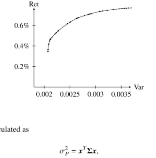
whereA=−u00(µP)/u0(µP) is Arrow’s absolute risk aversion (Arrow,1965). By “equivalent” we mean that maximizing (1) and (2) yield the same solutions. Substitutingλµ=2/Aand multiplying (2) byλµ, we have2 Ψ(µP, σ2P, λµ)=−σ2P+λµµP. (3) In (3),λµrepresents the risk tolerance of the investor regarding expected return. Varying the risk tolerance parameterλµover the nonnegative portion of the real line and maximizingΨcauses expected utility to yield the Markowitz nondominated frontier in variance-expected return space as in Figure1. It is to be noted that the nondominated frontier is segment-wise parabolic. That is, it is made up of a connected collection of parabolic segments. The dots in Figure1along the nondominated frontier are where the different parabolic segments connect with one another.
Since expected utilityΨcannot explain why certain investors would specifically choose SR mutual funds, it is suggested byBollen(2007) andDerwall et al.(2011, and references therein) that these investors also obtain utility from the social component of their investments. Furthermore,Ballestero et al.(2012) develop a financial-ethical model to select optimal portfolios for SR funds based on the three criteria of expected return, variance of return, and risk aversion. They use the concept of stochastic goal programming (Ballestero,2001) to incorporate an ethical goal into the framework of classical utility theory under uncertainty.
As discussed earlier, we confine the general Bernoulli decision theory setting (1) to a mean-variance setup (3). Here, expected portfolio return is calculated as
µP =µTx
2As a technical note, this transformation requiresu00 ,0. However, for risk-averse investors,u00 <0 always holds due to the concavity ofu.
Figure 1:A bi-criterion nondominated frontier. It is composed of a connected collection of parabolic segments. The frontier shown is from a bi-criterion problem withn =50 securities and has 46 segments.
0.002 0.0025 0.003 0.0035 0.2%
0.4%
0.6%
Var Ret
and portfolio variance is calculated as
σ2P =xTΣx,
where xis a portfolio composition vector (elements sum to one),µis a vector of individual security expected returns, andΣis ann×ncovariance matrix. As usual,xT symbolizes the transpose vectors ofx.
We now temporarily consider the approach ofBollen(2007) who proposes addingλννP to the expected utility expression of (3) whereνP is a simple indicator function equaling one if a portfolio satisfies the investor’s requirement for social responsibility. However, this makesνP a subjective quantity depending on each investor’s perception. Therefore, we strive for a more objective measure ofνPand feel that the social component is to be taken into account more appropriately in an investor’s expected utility function by the continuous quantity
νP =νTx
whereνis a vector of individual security ESG-scores. While the future ESG-score of a portfolio could be interpreted as a stochastic quantity, we consider in this paper the ESG-score to be deterministic. Hence, in updating (3) to account for social responsibility, we now have for expected utility
Φ(x,Σ,µ,ν, λµ, λν)=−σ2P+λµµP+λννP
=−xTΣx+λµµTx+λννTx (4)
whereλν is the risk tolerance of the investor regarding social responsibility.
Varying the risk tolerance pair (λµ, λν) over the nonnegative portion ofR2(which we callparameter space)
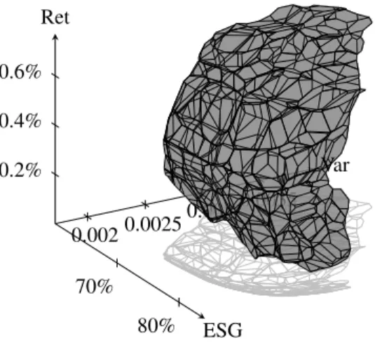
and maximizingΦcauses expected utility to yield, in contrast to the nondominated frontier, a nondominated surface in variance-expected return-ESG space as in Figure2. In particular, maximizingΦforλµ → ∞(while keepingλνfixed) yields a maximum expected return portfolio, and maximizingΦforλν→ ∞(while keeping λµfixed) yields a maximum ESG portfolio. It is to be noted that the nondominated surface is platelet-wise paraboloidic. That is, it is made up of a connected collection of (curved) paraboloidic platelets. The lines on the surface show where the different paraboloidic platelets abut one another.
Whereas, sinceMarkowitz(1956), it has been possible to compute a nondominated frontier as in Figure1, it has not been until recently, namely byHirschberger et al.(2013), that it has been possible to compute a tri-criterion nondominated surface as in Figure2. Using the CIOS (Custom Investment Objective Solver) code fromHirschberger et al.(2013) to solve for the tri-criterion nondominated surface, we are able to obtain from its output, for each paraboloidic platelet, (a) the platelet’s 2-dimensional polyhedron of (λµ, λν) vectors in parameter space and (b) the platelet’s polyhedron of efficient portfolio composition vectors in decision space. Recall that a point isefficientif and only if its image in criterion space is nondominated (where a point isnondominatedif and only if it is impossible to move from it to another without at least deteriorating one criterion).
Figure 2:A tri-criterion nondominated surface. Note that while a nondominated frontier is composed of a connected collection of parabolic segments, a nondominated surface is composed of a connected collection of paraboloidic “platelets.” The surface shown is from a tri-criterion problem withn=50 securities and has 1,460 platelets.
70%
80%
0.002 0.00250.003 0.0035 0.2%
0.4%
0.6%
ESG
Var Ret
To conclude the section, we wish to discuss on a few general issues that one might come up with when considering expected utilityΦfrom equation (4).
1. Notice that the concept of the rate of substitution for two objectives (seeKrugman & Wells,2009;
Pindyck & Rubinfeld,2005) is not general enough to consider indifference curves of constant utility
depending on variance, expected return and level of social responsibility. As both expected return and social responsibility are linear objectives, their marginal rate of substitution appears to be linear, but this is only true if variance is zero. If variance is positive the indifference curves follow the exact differential equation
0= ∂Φ
∂µP
dµP+ ∂Φ
∂νP
dνP+ ∂Φ
∂σ2Pdσ2P.
Here, the left hand side is zero since the marginal utility of the entire utility function does not change on a fixed indifference curve. Clearly, the rate of substitution in the values of expected return and social responsibility is linear, since both functions are linear in the portfolio weights. However, the change of portfolio weights also affects the variance of the portfolio, which is quadratic in the portfolio weights.
Hence, given a fixed level of variance, the expected return/ESG-score indifference curve is not linear.
2. Our setting allows that risk aversion depends on initial wealth. More precisely, the level of risk tolerance depends on the level of the initial wealth due to the fact that each decision maker chooses an efficient portfolio which is appropriate to her risk appetite according to both linear objectives as well as her level of initial wealth.
3. When considering equation (3) in the case of a risk-free investmentRf, the expected utilityΨ =λµRf
depends on the risk toleranceλµ. On first glance, this might seem counter-intuitive, since in equation (2) the equivalent expected utility ˆΨ = Rf was fixed for risk-free investments. However, notice that equation (2) does not denote the investor’s expected utility directly, but is an equivalent utility function when it comes to maximizing the expected utility (1). In fact, according to equation (1), the expected utility of a risk-free investment isE[u(Rf)]=u(Rf) (see for instanceCopeland et al.,2005, Chapter 3), which also depends on the investor’s individual utility function.
3. Inverse Optimization Process
For the experiments of this paper, inverse optimizations are needed to compute the values of the risk tolerance parametersλµ andλνthat areimpliedby a given fund’s portfolio composition vector on a given date (subsequently called a reporting date). In regular optimization, there is an objective function whose parameters are all fixed. Then we find the point in decision space that optimizes it. In inverse optimization, we start with a point in decision space. Usually, this point, which we designatew, is not efficient. Then the endeavor is to identify the efficient point that is closest towas a proxy point. Continuing, we then try to find what the values of certain parameters in the objective function would have to be for the proxy point to optimize the objective function. Strictly speaking, these are the parameters of the closest efficient point only, but they are then considered to be theimpliedparameters forw. The parameter values we are looking for in this paper are theλµandλν inΦ. Because theλµandλν of a portfolio cannot be computed directly, inverse portfolio optimization is used, which here involves the following steps:
1. Start with a given fund’s portfolio composition vectorwon a given reporting date.
2. Compute for the given fund on the given date its tri-criterion (financial variance-reward-ESG) nondom- inated surface, designated ˜E.
Here, we make two assumptions before calculating the nondominated surface. One is that the assets a fund is invested in on a given reporting date comprise all of the assets that the fund can actually invest in at that time. for the asset allocation. The other is that due to risk control, the fund enforces a minimal and maximal investing rule. That is, for the calculation of the nondominated surface there is a minimum and maximum amount that can be invested in each asset. These amounts are given by the actual individual minimum and maximum investments of the fund, i.e., by minj{wj}and maxj{wj}. Therefore, the nondominated surface for a given vectorwconsists of the images of all efficient portfolios that are achievable with the given assets present inwand under the aforementioned minimum and maximum constraints.
We use the CIOS algorithm to compute the nondominated surface. As an output from CIOS, we obtain information about all of the efficient polyhedra in decision space whose images form the platelets which together form the nondominated surface in criterion space.
3. Now, from the set of all efficient portfolio composition vectorsE, we need to find in decision space thex∈ Eclosest (in Euclidean norm) tow. We start by first comparing all of the vertices of all of the efficient polyhedra in decision space withw. We only work with vertices at this point because in the output of CIOS, the polyhedra of efficient portfolio composition vectors are only characterized by their vertices.
4. After finding theclosest vertex, we determine all of the polyhedra of efficient portfolio composition vectors (ascertainable from the output of CIOS) that are incident to this vertex (i.e., all polyhedra that have the “closest vertex” as one if its vertices).
5. Pixelate the polyhedron in (λµ, λν) parameter space associated with each polyhedron of efficient portfolio composition vectors identified in the above step. Utilizing the relationship inHirschberger et al.(2013) that enables us to specify thex∈ Efor each point in (λµ, λν) parameter space, we are able to pixelate all incident polyhedra inE.
6. Compare each pixelated point inx-space withw.
7. Then the point in parameter space associated with the pixelated x-vector that is closest (in Euclidean norm) towyields the desiredλµandλνimplied risk tolerance values.
Given a fund containingnsecurities, the inverse optimization process is expressed mathematically as
minλµ,λνkx−wk
s.t. x∈ E(λµ, λν) (5)
whereE(λµ, λν) is the solution of
maxx Φ(x,Σ,µ,ν, λµ, λν) (6a)
s.t. Pn
i=1xi =1 (6b)
xi≥min
j {wj} for alli (6c)
xi ≤max
j {wj} for alli (6d)
With regard to the outer minimization problem (5), note that the inner maximization problem (6a)–(6d) is a scalarized version of the actual tri-criterion portfolio selection model
minxTΣx max xTµ max xTν s.t. Pn
i=1xi =1 xi≥min
j {wj} for alli xi ≤max
j {wj} for alli
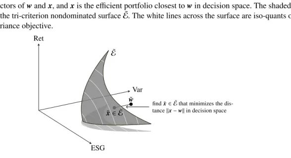
that we have been alluding to all along. The solutionxof the outer minimization problem (5) is the efficient portfolio corresponding to portfoliow. Figure3displays the procedure of inverse optimization graphically.
Notice that according to equation (4), the nondominated surfaceE(λµ, λν) could also be computed by solving a family of quadratic programs. One possibility would be the weighting method, where (6a)–(6d) is solved for many (λµ, λν) pairs. Another would be to use theε-constrained method, where the portfolio variance is minimized for a given level of expected return and a given level of ESG-score. While there has been some progress on improving the performance of theε-constrained method (Hamacher et al.,2007), the accuracy of an inverse portfolio optimization still critically depends on the accuracy of the generated nondominated surface. Yet, in order to obtain a reasonable degree of accuracy for the nondominated surface, it would have to be pixelated to the extent of at least several thousand points thus requiring that many quadratic programs to be solved to generate a single nondominated surface. Since we calculate more than 23,000 nondominated surfaces in total (see Section4), such a direct approach we require the solution of upwards of 50 million quadratic programming problems.
Figure 3:A picture illustrating the inverse portfolio optimization process where ˜wand ˜xare the criterion vectors ofwandx, andxis the efficient portfolio closest towin decision space. The shaded area is the tri-criterion nondominated surface ˜E. The white lines across the surface are iso-quants of the variance objective.
x˜ ∈E˜ w˜ E˜
find ˜x∈E˜that minimizes the dis- tancekx−wkin decision space
ESG
Var Ret
4. Data and Summary Statistics
In this study, after computing returns from stock prices in Thomson Reuters Datastream, we use a rolling window approach where each window has a length of 120 months and ends on a date that a fund reports its portfolio composition. In particular, we perform an inverse portfolio optimization for each reported fund composition and compute the one-month out-of-sample returns, i.e., the returns one month after the reported fund composition, both for the fund’s portfolio and for its respective efficient portfolio.
As for ESG-scores, they are based on actions already implemented in an observed company as well as on planned or started programs regarding the socially responsible performance of a company. Consequently, an ESG-score obtained from existing data at the end of monthtis an appropriate proxy for the socially responsible performance in montht+1.
The mutual fund compositions, which constitute the main information needed for the inverse optimizations are derived from the CRSP Survivor-Bias-Free US Mutual Fund database over the period December 31, 2001 to February 27, 2010. In contrast to returns, data on mutual fund compositions are typically not available more frequently than quarterly, with the dates on which composition information is reported called, as referred to earlier,reporting dates. Because of incomplete ESG data over the period of the study, certain funds are dropped. If it is not possible to obtain ESG-scores covering over 70% of a fund’s portfolio, the fund is dropped. Finally, we filter out all funds withn < 10 orn > 150 securities. For identifying which are SR mutual funds, we utilize the classifications of the U.S. Social Investment Forum (SIF)3. This then leaves us
3SIF provides a list with all known, socially responsible screened mutual funds online at the US SIF website athttp://ussif.org/
resources/mfpc/screening.cfm.
with 27 SR mutual funds and 2,346 conventional mutual funds. For the 27 SR mutual funds, we have a total of 276 different portfolio compositions over the different reporting dates. For the 2,346 conventional mutual funds, we have a total of 22,746 different portfolio compositions over the different reporting dates.
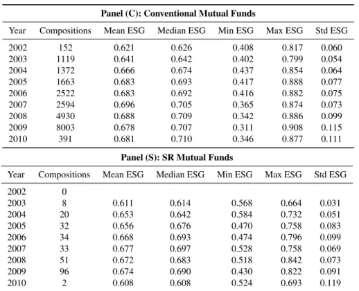
Table 1:Summary ESG statistics for conventional and socially responsible mutual funds.
Panel (C): Conventional Mutual Funds
Year Compositions Mean ESG Median ESG Min ESG Max ESG Std ESG
2002 152 0.621 0.626 0.408 0.817 0.060
2003 1119 0.641 0.642 0.402 0.799 0.054
2004 1372 0.666 0.674 0.437 0.854 0.064
2005 1663 0.683 0.693 0.417 0.888 0.077
2006 2522 0.683 0.692 0.416 0.882 0.075
2007 2594 0.696 0.705 0.365 0.874 0.073
2008 4930 0.688 0.709 0.342 0.886 0.099
2009 8003 0.678 0.707 0.311 0.908 0.115
2010 391 0.681 0.710 0.346 0.877 0.111
Panel (S): SR Mutual Funds
Year Compositions Mean ESG Median ESG Min ESG Max ESG Std ESG
2002 0
2003 8 0.611 0.614 0.568 0.664 0.031
2004 20 0.653 0.642 0.584 0.732 0.051
2005 32 0.656 0.676 0.470 0.758 0.083
2006 34 0.668 0.693 0.474 0.796 0.099
2007 33 0.677 0.697 0.528 0.758 0.069
2008 51 0.672 0.683 0.518 0.842 0.073
2009 96 0.674 0.690 0.430 0.822 0.091
2010 2 0.608 0.608 0.524 0.693 0.119
In Table1we list, by year, the number of different portfolio compositions, the mean portfolio ESG-score, median portfolio ESG-score, minimum portfolio ESG-score, maximum portfolio ESG-score, and the standard deviation of the different portfolio composition ESG-scores. A fund’s composition is included in a given year depending upon the date a change in composition is reported. Note that the average mean and average maximum ESG-scores of the SR mutual funds do not exceed those of the conventional mutual funds for all years. Nevertheless, the average minimum ESG-scores of SR mutual funds – that an SR investor would suppose to be higher – are indeed higher than those of conventional mutual funds. As the totals of SR mutual funds in 2002 and 2010 are 0 and 2, respectively, we do not consider these two years furthermore.
5. Hypothesis Development
In this section, we develop testable hypotheses regarding the investment policies of SR mutual funds. While the first two hypotheses consider the actual level of social responsibility of a fund, the next four hypotheses regard solely financial performance.
As already hinted above, asset allocation in a SR mutual fund is typically conducted in a two-stage approach. In the first stage, a set of suitable assets is selected by some kind of screening of all available assets, which is a binary selection process of the assets an investor is willing to buy. Among the criteria for the screening process can be requirements about the size and liquidity of a stock, or certain predefined standards regarding social responsibility (seeRenneboog et al.,2008). In the second stage, the fund manager then allocates the fund’s total wealth to the selected assets. We wish to analyze whether this asset allocation ignores social responsibility, i.e., is influenced only by the expected returns and the covariances of the returns, or whether social responsibility is taken into account in the second stage, too.
Hypothesis 1a: Asset allocation after screening in SR mutual funds depends upon the social responsibility of the individual assets.
Hypothesis 1a is about whether ESG-scores continuing to play a role in the asset allocation of the second stage, i.e., after the screening process has been conducted. Notice that the importance of the ESG-score in the second-stage asset allocation is measured by the implied risk tolerance with respect to the ESG-scoreλν. For instance, small values ofλνindicate that fund managers weight the ESG-scores only marginally, whereas a highλνindicates a high appreciation of the ESG-scores.
Consequently, it can be asked (below) whether the ESG-scores of SR mutual fund portfolios exceed those of their conventional peers.
Hypothesis 1b: SR mutual funds show higher weighted ESG-scores than conventional mutual funds.
A high ESG-score can be explained either by the screening process or by giving assets with high ESG-scores more weight in a fund’s portfolio, i.e., by operating with a higher risk toleranceλν.
Having challenged funds’ abilities to incorporate ESG-scores into their asset allocations, we now continue with hypotheses about their skills in generating financial performance. The financial performance of SR mutual funds is a heavily discussed area in literature (seeBauer et al.,2005;Bello,2005;Guerard,1997;
Hamilton et al.,1993;Kreander et al.,2005;Mallin et al.,1995;Statman,2000). We compare the implied financial risk tolerances, the overall returns, the overall risks (which we measure in terms of standard deviation), and the out-of-sample returns of the conventional and SR mutual funds.
Hypothesis 2a: SR mutual funds differ from conventional mutual funds in terms of financial risk tolerance.
Hypothesis 2b: SR mutual funds show lower returns than conventional mutual funds.
Hypothesis 2c: SR mutual funds differ from conventional mutual funds in terms of risk.
Hypothesis 2d: SR mutual funds differ from conventional mutual funds in terms of out-of-sample return.
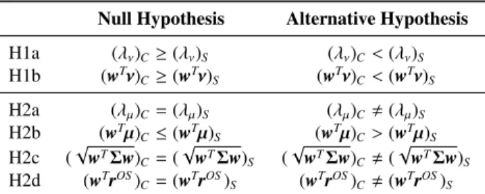
Table2formally summarizes the hypotheses from above. As for notation, in line H1a, the Alternative Hypothesis is that the risk tolerance parameter regarding social responsibility is higher in SR mutual funds than in conventional mutual funds. As another example, in line H2d, the Null Hypothesis is that the out-of- sample returns of conventional mutual funds are equal to the out-of-sample returns of the actual portfolios of SR mutual funds.
Table 2:Test hypotheses.
Null Hypothesis Alternative Hypothesis H1a (λν)C≥(λν)S (λν)C<(λν)S
H1b (wTν)C≥(wTν)S (wTν)C<(wTν)S
H2a (λµ)C=(λµ)S (λµ)C,(λµ)S
H2b (wTµ)C≤(wTµ)S (wTµ)C>(wTµ)S
H2c (√
wTΣw)C=(√
wTΣw)S (√
wTΣw)C,(√ wTΣw)S
H2d (wTrOS)C=(wTrOS)S (wTrOS)C,(wTrOS)S
6. Results
Using a rolling window approach, the latest available ESG-scores before a reporting date, the inverse portfolio optimization process, and out-of-sample returns, we now have, for our hypothesis testing, the descriptive statistics of Table3. This table and the following tests are based on the computation of an inverse optimization for each of the 23,022 different fund compositions reported above.
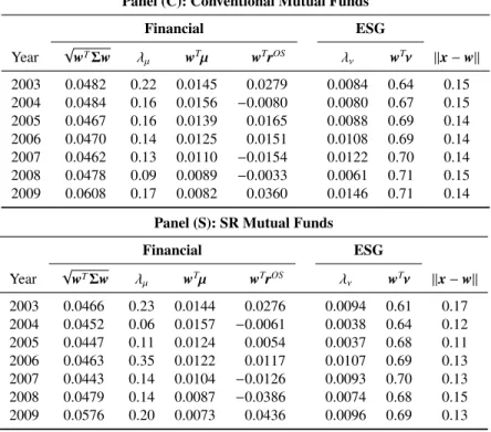
Continuing with the notation that x is an efficient portfolio andwis an already existing mutual fund portfolio, we now have by year, in Table3, median values for portfolio in-sample volatility4, implied financial risk tolerance, monthly portfolio in-sample returns, and monthly portfolio out-of-sample returns. Also, we have median values for implied socially responsible risk tolerance, and in-sample portfolio ESG-scores. In the last column of the table we have median values for the distances between thex’s and theirw’s in our experiments.
Especially for the impliedλν andλµ, the median is a more appropriate statistic than the mean to depict the data in a single quantity because of skewness and outliers. Even so, the mean values (not reported) of the empirical distributions of all columns, apart from those of the two implied risk tolerances, do not differ much from the reported medians anyway. The implied risk tolerance parametersλµandλνrange between 0 and 13,112 (λµ), and 0 and 2,215 (λν), respectively. However, the informative value of these intervals is rather limited due to the fact that the level of the risk tolerance parameters depends on the scale ofµandνas well as on the specification of the utility function (seeKallberg & Ziemba,1983, for an extensive discussion).
4We report volatility in opposite to variance in the remainder of this section since volatility is given in the same unit (percent per month) as return.
Table 3:Descriptive statistics for use in hypothesis testing.
Panel (C): Conventional Mutual Funds
Financial ESG
Year √
wTΣw λµ wTµ wTrOS λν wTν kx−wk 2003 0.0482 0.22 0.0145 0.0279 0.0084 0.64 0.15 2004 0.0484 0.16 0.0156 −0.0080 0.0080 0.67 0.15 2005 0.0467 0.16 0.0139 0.0165 0.0088 0.69 0.14 2006 0.0470 0.14 0.0125 0.0151 0.0108 0.69 0.14 2007 0.0462 0.13 0.0110 −0.0154 0.0122 0.70 0.14 2008 0.0478 0.09 0.0089 −0.0033 0.0061 0.71 0.15 2009 0.0608 0.17 0.0082 0.0360 0.0146 0.71 0.14
Panel (S): SR Mutual Funds
Financial ESG
Year √
wTΣw λµ wTµ wTrOS λν wTν kx−wk 2003 0.0466 0.23 0.0144 0.0276 0.0094 0.61 0.17 2004 0.0452 0.06 0.0157 −0.0061 0.0038 0.64 0.12 2005 0.0447 0.11 0.0124 0.0054 0.0037 0.68 0.11 2006 0.0463 0.35 0.0122 0.0117 0.0107 0.69 0.13 2007 0.0443 0.14 0.0104 −0.0126 0.0093 0.70 0.13 2008 0.0479 0.14 0.0087 −0.0386 0.0074 0.68 0.15 2009 0.0576 0.20 0.0073 0.0436 0.0096 0.69 0.13
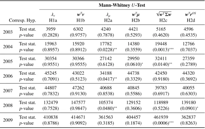
As mean values of the parameters could be biased by outliers, we test our hypotheses using the non- parametric Mann-WhitneyU-Test. We report the test statistics and the corresponding p-values of each test in Table4.
The parametersλµ andλν display the implied risk tolerances, which we compute via inverse portfolio optimization as described earlier. Since the two risk tolerance parameters are computed from the efficient portfoliosxrather than from the funds’ real portfoliosw, one could be fearful that the implied parameters do not reflect the funds’ actual parameters reasonably well. However, when considering the distanceskx−wk reported in Table3, we see that the two fund compositions do not differ a lot.
Generally, zero values forλµ orλν imply infinite risk aversion. By this we mean that no efforts will be made to increase expected return (in the case ofλµ=0) or ESG-score (in the case ofλν =0) if it comes at the expense of increasing risk above its minimal value. While a few funds exhibit a zeroλµ or a zeroλν, we see that most fund managers are willing to take on risk above the minimum to achieve additional expected return and/or higher ESG-scores, as the medians of bothλ’s are positive.
To determine whether screening is the only approach used to build SR mutual funds, we test to see if the implied tolerancesλν are greater in SR mutual funds than in conventional mutual funds. In principle, conventional mutual funds are to maximize expected utility containing only financial terms implying aλν of zero. However, conventional mutual funds may exhibit non-zero λν’s due to random noise stemming
Table 4:Test statistics andp-values for the hypotheses H1a–H2d of Table2where∗,∗∗,∗∗∗denote significant parameters at a 10%, 5%, and 1% level, respectively.
Mann-WhitneyU-Test
λν wTν λµ wTµ √
wTΣw wTrOS
Corresp. Hyp. H1a H1b H2a H2b H2c H2d
2003 Test stat. 3959 6302 4240 4421 5165 4596
p-value (0.2828) (0.9757) (0.7878) (0.5293) (0.4620) (0.4535)
2004 Test stat. 15963 15920 17782 14380 19448 12766
p-value (0.8957) (0.8912) (0.0228)∗∗ (0.3559) (0.0013)∗∗∗ (0.7037)
2005 Test stat. 30354 30366 27142 29950 32411 27359
p-value (0.9551) (0.9555) (0.6128) (0.0610)∗ (0.0140)∗∗ (0.2789)
2006 Test stat. 45245 43022 34188 44738 42450 44320
p-value (0.7091) (0.5123) (0.0417)∗∗ (0.3329) (0.9180) (0.3692)
2007 Test stat. 44807 47262 40688 40845 39783 40055
p-value (0.7832) (0.9130) (0.8538) (0.5586) (0.6917) (0.6303)
2008 Test stat. 132479 147577 105374 129152 118989 139180
p-value (0.7528) (0.9847) (0.0480)∗∗ (0.3606) (0.5226) (0.0901)∗
2009 Test stat. 410838 414671 361563 404457 461939 362837
p-value (0.8786) (0.9092) (0.3185) (0.1874) (0.0006)∗∗∗ (0.8263) from the inverse optimizations. If SR mutual funds value assets with high ESG-scores more, then we would expect theirλν’s to exceed the randomλν’s of their conventional counterparts. Yet, we find no statistically significant evidence to reject the null hypothesis of H1a in any year. Therefore, we cannot confirm that managers of SR mutual funds pursue any socially responsible strategies in their second-stage asset allocations that conventional fund managers do not. This is in clear contrast to the common investor opinion that SR mutual funds would not be disregarding social responsibility issues after their initial screenings have been made. Next, we test whether there are any differences in the socially responsible performance of the two types of funds at all. Since we have already found that SR mutual funds do not show higher risk tolerances with respect to social responsibility, higher ESG performances had to be attributed to the screening processes.
However, we cannot reject the null of H1b at any arbitrary confidence level. Therefore, our data suggest that SR mutual funds do not exhibit higher ESG-scores than conventional mutual funds.
With regard to the commonly used term of financial risk tolerance displayed asλµ, we investigate H2a, but we find no strong evidence with the Mann-WhitneyU-Test in any year that there is a difference between the λµ’s of the SR mutual funds and the conventional funds. Nevertheless, we find some evidence to reject the null in the years 2004, 2006 and 2008, which indicates that the financial risk tolerance of conventional and
SR mutual funds differ in those years.
Adler & Kritzman(2008) andDorfleitner & Utz(2012) show that building portfolios in which ESG-score is an objective yields a decrease in returns relative to portfolios where social responsibility is of only minor importance. Following this result, we test in H2b whether the returns of SR mutual funds are significantly lower than the returns of conventional funds. Apart from weak empirical evidence to reject the null in 2005, we do not find any statistical evidence in other years. This indicates that we cannot reject the null hypothesis, which states that the distribution function of the portfolio return of the conventional mutual funds is not significantly higher than that of the SR mutual funds, at any arbitrary significance level. Therefore, we are in line with several former studies (Bauer et al., 2005;Bello, 2005;Guerard,1997;Hamilton et al., 1993;Kreander et al.,2005;Mallin et al.,1995;Statman,2000) that find no significant differences in fund performance between conventional and SR mutual funds.
We also test the standard deviations of the mutual funds and find that the null of H2c can be rejected at the 1% significance level in 2004 and 2009 and at the 5% significance level in 2005. Thus, in our sample, conventional mutual funds differ with some significance from SR mutual funds in terms of standard deviation.
Moreover, the data in Table3show that the standard deviations of conventional mutual funds are at least as high as the standard deviations of SR mutual funds in all years but 2008.
The out-of-sample fund returns, which describe real fund performance in the month following the date of portfolio composition, are tested in H2d. We check whether the distribution of one-month out-of-sample returns of conventional mutual funds differs from the distribution of one-month out-of-sample returns of SR mutual funds. We do not find any statistical evidence to reject the null. Thus, we cannot conclude that there are statistically significant differences between the two respective distributions.
Summarizing the results of Table4, we cannot find any statistical evidence that implies profound differences between conventional and SR mutual funds. Furthermore, we check the robustness of our results. With regard to supposed sensitivity of the results of a Markowitz model to its input parameters (see for exampleFabozzi et al.,2002), we apply different methods for estimating (i.e., exponentially weighted moving average) the financial parameters and we also vary the time period upon which the estimation is based. In summary, we do not find any profound differences in the tests’ results.
7. Summary and Conclusion
In this article, we present a framework for inverse portfolio optimization in a Markowitz model, which is extended to include a third criterion. Using the prescribed inverse optimization process we are able to compute the implied risk tolerance parameters of mutual funds that pursue a third, non-financial criterion.
In applying this capability to a broad sample of conventional and socially responsible (SR) mutual funds, we find that after the screening process there appears to be no significant difference in how assets are allocated in socially responsible and conventional mutual funds. By considering the implied risk tolerance with respect to the ESG-score, we are unable to find evidence that social responsibility is taken into account in the asset
allocation stage at all. With regard to key indicators such as volatility, expected return, and ESG-scores (used to measure social responsibility), we find a slightly lower volatility for the SR mutual funds’ returns, but we find no significant differences for the expected return and the mean ESG-scores.
The methodological ideas developed in this paper pave the ground to various new research. For instance, the approach is not bound to the application of SR mutual funds. Applying a tri-criterial model to other real-world problems might be of interest both for practitioners and the scientific community. Moreover, while the decision model in the inverse optimization in this paper was tri-criterial, further research could broaden the model to include more than three criteria.
References
Abdelaziz, F. B., Aouni, B., & Fayedh, R. E. (2007). Multi-objective stochastic programming for portfolio selection. European Journal of Operational Research,177, 1811–1823.
Adler, T., & Kritzman, M. (2008). The cost of socially responsible investing.Journal of Portfolio Management, 35, 52–56.
Arrow, K. (1965). Aspects of the Theory of Risk Bearing. Academic Book Store, Helsinki.
Ballestero, E. (2001). Stochastic goal programming: A mean–variance approach. European Journal of Operational Research,131, 476–481.
Ballestero, E., Bravo, M., P´erez-Gladish, B., Arenas-Parra, M., & Pl`a-Santamaria, D. (2012). Socially responsible investment: A multicriteria approach to portfolio selection combining ethical and financial objectives. European Journal of Operational Research,216, 487–494.
Bauer, R., Koedijk, K., & Otten, R. (2005). International evidence on ethical mutual fund performance and investment style. Journal of Banking and Finance,29, 1761–1767.
Bello, Z. Y. (2005). Socially responsible investing and portfolio diversification. The Journal of Financial Research,28, 41–57.
Bierwag, G. O. (1974). The rationale of the mean-standard deviation analysis: Comment.American Economic Review,64, 431–433.
Bollen, N. P. B. (2007). Mutual fund attributes and investor behavior. Journal of Financial and Quantitative Analysis,42, 683–708.
Chamberlain, G. (1983). A characterization of the distributions that imply mean–variance utility functions.
Journal of Economic Theory,29, 185–201.
Copeland, T. E., Weston, J. F., & Shastri, K. (2005).Financial Theory and Corporate Policy. Pearson, Boston, Massachusetts.
Derwall, J., Koedijk, K., & Horst, J. T. (2011). A tale of values-driven and profit-seeking social investors.
Journal of Banking and Finance,35, 2137–2147.
Dorfleitner, G., Leidl, M., & Reeder, J. (2012). Theory of social returns in portfolio choice with application to microfinance. Journal of Asset Management,13, 384–400.
Dorfleitner, G., & Utz, S. (2012). Safety first portfolio choice based on financial and sustainability returns.
European Journal of Operational Research,221, 155–164.
Fabozzi, F. J., Gupta, F., & Markowitz, H. M. (2002). The legacy of modern portfolio theory. Journal of Investing,11, 7–22.
Feldstein, M. S. (1969). Mean-variance analysis in the theory of liquidity preference and portfolio selection.
Review of Economic Studies,36, 5–12.
Guerard, J. B. (1997). Additional evidence on the cost of being socially responsible in investing. Journal of Investing,6, 31–36.
Haimes, Y. Y., Lasdon, L. S., & Wismer, D. A. (1971). On a bicriterion formulation of the problems of integrated system identification and system optimization. IEEE Transactions on Systems, Man and Cybernetics,SMC-1, 296–297.
Hallerbach, W., Ning, H., Soppe, A., & Spronk, J. (2004). A framework for managing a portfolio of socially responsible investments. European Journal of Operational Research,153, 517–529.
Hamacher, H. W., Pedersen, C. R., & Ruzika, S. (2007). Finding representative systems for discrete bicriterion optimization problems. Operations Research Letters,35, 336–344.
Hamilton, S., Jo, H., & Statman, M. (1993). Doing well while doing good? The investment performance of socially responsible mutual funds. Financial Analysts Journal,49, 62–66.
Hirschberger, M., Steuer, R. E., Utz, S., Wimmer, M., & Qi, Y. (2013). Computing the nondominated surface in tri-criterion portfolio selection. Operations Research,forthcoming.
Kallberg, J. G., & Ziemba, W. T. (1983). Comparison of alternative utility functions in portfolio selection problems. Management Science,29, 1257–1276.
Kreander, N., Gray, R., Power, D., & Sinclair, C. (2005). Evaluating the performance of ethical and non-ethical funds: A matched pair analysis. Journal of Business Finance and Accounting,32, 1465–1493.
Krugman, P., & Wells, R. (2009). Microeconomics. Worth Publishers, New York.
Levy, H. (1974). The rationale of the mean-standard deviation analysis: Comment. American Economic Review,64, 434–441.
Mallin, C., Saadouni, B., & Briston, R. (1995). The financial performance of ethical investment funds.
Journal of Business Finance and Accounting,22, 483–496.
Markowitz, H. M. (1952). Portfolio selection. Journal of Finance,7, 77–91.
Markowitz, H. M. (1956). The optimization of a quadratic function subject to linear constraints. Naval Research Logistics Quarterly,3, 111–133.
Markowitz, H. M. (1959). Portfolio Selection: Efficient Diversification of Investments. John Wiley and Sons, New York.
Markowitz, H. M. (1987).Mean-Variance Analysis in Portfolio Choice and Capital Markets. Basil Blackwell, Oxford.
Markowitz, H. M., & Todd, P. (2000). Mean-Variance Analysis in Portfolio Choice and Capital Markets. Frank J. Fabozzi Associates, New Hope, Pennsylvania.
von Neumann, J., & Morgenstern, O. (1947).Theory of Games and Economic Behaviour. (2nd ed.). Princeton University Press, Princeton, New Jersey.
Pindyck, R., & Rubinfeld, D. (2005). Microeconomics. Pearson Prentice Hall, Upper Saddle River, New Jersey.
Pratt, J. W. (1964). Risk aversion in the small and in the large. Econometrica,32, 122–136.
Renneboog, L., Horst, J. T., & Zhang, C. (2008). Socially responsible investments: Institutional aspects, performance, and investor behavior. Journal of Banking and Finance,32, 1723–1742.
Statman, M. (2000). Socially responsible mutual funds.Financial Analysts Journal,56, 30–38.
Steuer, R. E., Qi, Y., & Hirschberger, M. (2007). Suitable-portfolio investors, nondominated frontier sensitivity, and the effect of multiple objectives on standard portfolio selection. Annals of Operations Research,152, 297–317.
Tobin, J. (1969). Comment on Borch and Feldstein. Review of Economic Studies,36, 13–14.
Tsiang, S. C. (1972). The rationale of the mean-standard deviation analysis, skewness preference, and the demand for money. American Economic Review,62, 354–371.
Xidonas, P., & Mavrotas, G. (2012). Multiobjective portfolio optimization with non-convex policy constraints:
Evidence from the Eurostoxx 50. European Journal of Finance,forthcoming.
Xidonas, P., Mavrotas, G., Krintas, T., Psarras, J., & Zopounidis, C. (Eds.) (2012). Multicriteria Portfolio Management. Springer, New York.
Zagst, R., & P¨oschik, M. (2008). Inverse portfolio optimisation under constraints. Journal of Asset Management,9, 239–253.