vorgelegtvonDiplom-MathematikerinAngelikaDiesesausNeustadt/WeinstraßeTagdermündlichenPrüfung:15.Dezember2000 zurErlangungderDoktorwürdederNaturwissenschaftlich–MathematischenGesamtfakultätderRuprecht–Karls–UniversitätHeidelberg I –D

(1)

I

NAUGURAL

– D

ISSERTATION

zur

Erlangung der Doktorw ¨urde der

Naturwissenschaftlich–Mathematischen Gesamtfakult¨at der

Ruprecht – Karls – Universit¨at Heidelberg

vorgelegt von

Diplom-Mathematikerin Angelika Dieses aus Neustadt/Weinstraße

Tag der m ¨undlichen Pr ¨ufung: 15. Dezember 2000

(2)

(3)

Numerical Methods for Optimization Problems in Water Flow and Reactive Solute Transport Processes of Xenobiotics in Soils

Gutachter: Prof. Dr. Hans Georg Bock

Prof. Dr. Otto Richter

(4)

(5)

I

Acknowledgements

First and foremost, I wish to thank my advisors Prof. Dr. Hans Georg Bock, Interdisciplinary Center for Scientific Computing (IWR), University of Heidelberg, and Prof. Dr. Otto Richter, Institute of Geoecology, Technical University of Braunschweig, for their interest in planning and supervising this interdisciplinary project and for their continuous support during the last three years. In addition, I am greatly indebted to Dr. Johannes Schl¨oder, IWR, for many inspir- ing and fruitful discussions and for the excellent supervision he gave me all the time.

I wish to thank my colleagues in the group of Prof. Dr. Hans Georg Bock and Dr. Jo- hannes Schl¨oder for their friendship and their assistance. Without the advanced software and the enormous knowledge base available in the group, the development of the tools ECOFIT andECOPLANwould not have been possible in such a short period of time. In particular, I am indebted to Dr. Irene Bauer and Stefan K¨orkel for providing the software packagesDAESOL and VPLANand for various discussions about integration methods and optimal experimental design. I also thank my colleague and roommate Oliver Großhans for always having an open ear for my questions and for his friendly help with diverse soft- and hardware problems. In this context, I also want to mention the excellent environment and atmosphere of the IWR for doing interdisciplinary research.

I also would like to thank Prof. Dr. Otto Richter and all his co-workers, in particular Dr. Dag- mar S¨ondgerath, Dr. Ralf Seppelt and Michael Flake, for their warm welcome during my four months stay at their institute and for the introduction to the secrets of soil science and environmental fate modeling of xenobiotics.

Special thanks go to Dr. Anna Schreieck, Dr. Marite de Mehr and Prof. Dr. Josef Kallrath, BASF AG Ludwigshafen, and Dr. Bernhard Gottesb¨uren, BASF Agricultural Center Limburger- hof, for their interest in this project and for the financial support. The financial support granted by Deutsche Forschungsgemeinschaft, Sonderforschungsbereich 359, “Reaktive Str¨omungen, Diffusion und Transport” is also gratefully acknowledged.

I owe many thanks to Karin Aden and Andreas Horn, Institute of Geoecology, Technical University of Braunschweig, for the good cooperation and for their great effort to supply me with laboriously collected experimental data. I am grateful to the BASF Agricultural Center in Limburgerhof, the Staatliche Lehr- und Forschungsanstalt (SLFA) in Neustadt/Weinstr., and the Novartis Crop Protection AG in Basel for giving me access to interesting studies and experimental data.

And last, but certainly far from least, I thank my parents for their love and their continuous support during all the years of study, and my fianc´e Stephan for his love and his encouraging support while doing this PhD project.

(6)

(7)

List of Symbols

Lowercase Latin Characters concentration in the liquid phase

fixed reference concentration for Freundlich isotherm

total concentration

correction factor for the mass balance

concentration in the gaseous phase

acceleration of gravity

"! $#

%'&

degradation rate in the liquid phase

( $)

%'*

degradation rate in the solid phase

( $)

%

+ apparent rate constant

(,$)-

. ,

fitting parameters

/ volumetric water flux density

0( $)

!

concentration in the solid phase

$)

1 time

(2

3 pore water velocity

0(,$)-

4 conversion factor ^46587:9

"! $#

; vertical coordinate (positive downward)

<

Uppercase Latin Characters

=?>@BADC

specific soil water capacity in

@BA $) 0( #

=?>EFC

inverse of specific soil water capacity in

E

$)

(

$#

GIH

coefficient of molecular diffusion in pure water

# ( $)

GKJML

coefficient of molecular diffusion in the air

# ( $)

GKN

coefficient of molecular diffusion in the liquid phase

# ( $)

GKO

hydrodynamic dispersion term

# ( $)

G A

coefficient of dispersion

# ( $)

G *

coefficient of molecular diffusion in the gaseous phase

P#Q(,$)-

G >E C

soil water diffusivity

P#Q(,$)-

R &

mass flux due to convection

$#( $)

R N

mass flux in the liquid phase due to diffusion

$#

(

$)

R S

mass flux in the gaseous phase

$#Q(,$)

R A

mass flux in the liquid phase due to dispersion

$#( $)

VII

(12)

R

total mass flux

$# ( $)

T

>@UAVC

hydraulic conductivity in

@UA $) (2

T

>E C

hydraulic conductivity in

E

$) (2

TWN

equilibrium constant of linear isotherm

X$)Y0Z

T

sorption coefficient of Freundlich isotherm

\[ [

T

sorption coefficient of scaled Freundlich isotherm

$)

TW]

sorption coefficient of Langmuir isotherm

$)

T *

saturated hydraulic conductivity

$) (2

TW^

Michaelis constant

_

Freundlich exponent

`

source/sink term in the convection-dispersion equation

Y(,$)-

a

source/sink term in the Richards equation in

@UA

( $)

a

source/sink term in the Richards equation in^E

( $)

b A Jdc

maximal reaction velocity (Michaelis-Menten kinetics)

( $)

Lowercase Greek Characters

e fitting parameter

$) 0( #

egf dispersion length

<

e adsorption-desorption rate

( $)

h

finite adsorption capacity

$)

i volumetric air content

j

pore size distribution index

k

l

porosity of the soil

0Fm d

@Un

bubbling pressure

$)( $#

@ S

gravitational potential

$)( $#

@ O

soil water potential

$)( $#

@UA

matric potential

$)( $#

@ *

osmotic potential

$)( $#

@Uoqp

tensiometer potential

$)Q(,$#-

7 bulk density

7:9 mass density of water

E

volumetric water content

E

residual water content

E *

saturated water content

r

>EFC

tortuosity factor

k

Uppercase Greek Characters

s

normalized water content

k

(13)

Introduction

Xenobiotics such as pesticides, herbicides or fungicides, play a key role in an efficient and eco- nomic agriculture. Their critical impact on the environment, in particular on the groundwater, has long been recognized. In recent years, care about environmental effects and human safety has become of major public interest. Authorities have responded by introducing stricter reg- ulations and imposing stringent test procedures before releasing a substance for use in fields (Plimmer, 1999 [101]).

On the European level, the Registration Directive 91/414/EEC, concerning the placing of plant protection products (PPP) on the EU market, came into force in 1993 (Boesten et al., 1999 [24]). Uniform principles for the registration process, e.g. the type and scope of experimental studies, were defined. In particular, it is required that in addition to the experiments carried out for the assessment of the fate and behavior of plant protection products in the environment, estimates of predicted environmental concentrations in soil, water, and air based on mathematical modeling have to provided (Kloskowski et al., 1999 [73]). Several simulation tools, e.g. PELMO (Klein, 1995 [72]; Jene, 1998 [69]), PEARL (Tiktak et al., 1999 [125]), PRZM (Carsel et al., 1998 [29]) or MACRO (Jarvis and Larsson, 1998 [68]), have become available and are widely used by research institutes as well as companies and regulatory agencies. Devel- opments in recent years have shown that due to its enormous potential to predict the substance behavior for different soils and climatic conditions, mathematical modeling and simulation will be of increasing importance for the registration process.

In order to solve the simulation problem, i.e. the forward problem, for predicting system states, e.g. concentrations, the values of all parameters used in the mathematical model have to be available. Usually, the unknown parameters in the model, such as sorption coefficients or half-lifes, are determined from batch experiments or incubation studies using sieved soils under controlled temperature and moisture conditions in the laboratory. However, the validity of the extrapolation of laboratory data to transport and degradation processes in undisturbed soil cores or in the field have been questioned.

An alternative and very promising way to obtain parameters suitable for predicting the environmental fate of xenobiotics is inverse modeling. The idea of inverse modeling is to estimate the unknown parameters directly from lysimeter or field measurement data. This is done by mathematical optimization, where an objective function containing weighted deviation between the computed and the observed data is minimized.

1

(14)

Inverse modeling has been common practice for saturated flow problems in ground-water hydrology for years (Yeh, 1986 [142]). Its application to the unsaturated zone is relatively new.

It has thus far been mainly limited to the water transport equation to infer hydraulic parameters of the soil. For overviews see (Kool et al., 1987 [81]) and (Hopmans and ˇSim˚unek, 1999 [61]). There are only few papers considering parameter estimation for reactive solute transport under unsaturated conditions described by coupled water and solute transport equations (see e.g. Mishra and Parker, 1989 [92]; Medina and Carrera, 1996 [90]; Abbaspour et al., 1997 [1];

ˇSim˚unek and van Genuchten, 1999 [116]; Dieses et al., 1999 [41]; Dieses et al., 1999 [43]). In the context of registration studies, the idea has been pursued to compute unknown parameters by coupling simulation tools with commonly available nonlinear regression software, e.g. PEST (Doherty, 1994 [44]). However, the results thus obtained are mainly unsatisfying.

Up to now, the registration of new substances on the basis of parameters derived by inverse modeling has been granted only in some specific cases. However, the role of inverse modeling in the registration of plant protection products is under discussion. Members of different national authorities of European countries, e.g. Germany, Denmark, United Kingdom, The Netherlands, Belgium and France, gave statements on the current status of the use of inverse modeling in national pesticide registration at the recent “Workshop on Inverse Modeling” at the Research Center J¨ulich in May 2000. An expert of the German regulatory agency, the Biologische Bun- desanstalt f¨ur Land- und Forstwirtschaft (BBA), for example, stated that “up to now inverse modeling is a procedure that is not very well tested and accepted” and that “more information on the method is needed until it can be accepted.” In summary, there was no consensus as such. Even though the benefits were granted, the broad majority of the representatives expressed a rather cautious attitude towards the results obtained so far. Most adopted a policy of wait-and-see asking for more information and expertise in order to judge the method’s validity.

In particular, more sophisticated mathematical methods were required in order to overcome the deficiencies encountered by combining simulation models with model-independent nonlinear regression tools. The INRA, France, for example, claimed that “more insight into the tech- niques of inversion (feasibility, mathematical pitfalls, robustness of the method,...) is needed.”

However, in order to establish inverse modeling in the registration process, in addition to reliable tools for parameter estimation, optimized experimental designs for column, lysimeter and field experiments are necessary. Methods are needed to determine experimental conditions, such as irrigation or application schemes, and sampling designs leading to measurement data that is suitable for parameter estimation. The choice of the experimental design is of particular interest, as the parameter estimation problems investigated so far have frequently been shown to be ill-posed. Even though this problem of ill-posedness, mainly caused by parameters that are practically insensitive to the measurement data, has been encountered in many studies (e.g. Hornung, 1983 [63]; Kool et al., 1985 [80]; Toorman et al., 1992 [126]; van Dam et al., 1992 [127]), only a few approaches for optimizing the experimental designs have been reported.

In some few cases the problem to derive better experimental conditions and sampling schemes has been interpreted and formulated as a mathematical optimization problem. Due to the lack

(15)

Introduction 3

of suitable optimization procedures, the problem has often been solved by an enumerative grid search through the design space (e.g. Knopmann and Voss, 1987 [74]; 1989 [76]). Sun (1994 [123]) even stated that “in practice to solve such a general problem is too difficult” and “that up to date, only few hypothetical examples and simplified cases have been reported”.

Hence, in addition to the scientific interest there is an increasing demand by industry and also by national authorities for sophisticated and reliable methods for both parameter estimation and optimal experimental design in transport and degradation processes of xenobiotics in soils.

This is the background setting for this work which aims at providing methods that simplify investigations and enable a better understanding of the observed processes. In order to support the mathematical modeling, the toolsECOFIT(Dieses et al., 1999 [41]; 1999 [43]) for parameter estimation and ECOPLAN(Dieses et al., 2000 [42]) for optimal experimental design in water and reactive solute transport processes in soils have been developed. In this thesis new contributions are made to the following fields:

t Modeling of parameter estimation problems and optimal experimental design problems

t Numerical methods for parameter estimation in water flow and reactive solute transport processes of xenobiotics in soils

t Numerical methods for optimal experimental design in water flow and reactive solute transport processes of xenobiotics in soils

t Application of the developed methods to various real-life problems

In the following we give a summary containing the new contributions made to these topics.

We have organized this thesis in essentially independent chapters because we assume that not all readers are interested in all chapters to the same extent. Those readers who are mainly interested in the modeling aspects and in the application of the tools ECOFITand ECOPLAN to column, lysimeter and field studies are referred to the Chapters 1 and 5. For those readers who are interested in the mathematical part and want to get a deeper understanding of the multiple shooting method and the Generalized Gauss-Newton method, a review is provided in Section 2.1 and 2.2 based on (Bock, 1981 [19]; 1983 [20]; 1987 [21]; Schl¨oder and Bock, 1983 [109]; Schl¨oder, 1988 [108] ).

Modeling for Parameter Estimation and Optimal Experimental Design (Chapter 1) When studying the environmental fate of xenobiotics, the vadoze zone, i.e. the first 30 to 100 centimeters of the soil where the relevant processes such as degradation take place, is of particular interest. As this zone is generally not saturated with water, the transport of dissolved substances is greatly affected by the flow of water. Thus, unless studying column experiments in the laboratory where steady-state conditions can be met, the transport of both water and solute have to be considered simultaneously. The mathematical modeling of water and solute

(16)

transport processes in the unsaturated zone leads to instationary partial differential equations (PDEs) coupled with nonlinear ordinary differential (ODEs) or differential algebraic equations (DAEs).

For the sake of comparability and in order to enable the use of the developed tools for registration studies, the choice of model equations considered in this work is oriented at the equations implemented in the simulation models used so far for registration. In addition to these models, presented in Section 1.1 and 1.2, we investigate more complex models, not yet available in the commonly used simulation tools, that include e.g. nonlinear sorption described by Langmuir isotherms or nonlinear degradation according to Michaelis-Menten kinetics. A very difficult problem in the modeling of column, lysimeter or field experiments is the appropriate description of initial and boundary conditions. In Section 1.3, we summarize frequently encountered conditions in practice and work out suitable modeling approaches for initial, upper and lower boundary conditions.

Section 1.4 is devoted to the parameter estimation problem in environmental fate experiments. In Section 1.4.1, we present a formulation for the inverse problem that covers a wide range of typical column and lysimeter experiments. In Section 1.4.2, the parameter estimation methods used in common practice are reviewed and analyzed. In contrast to the frequently reported approach where the simulation and the optimization problems are treated separately, we pursue a different approach where the parameter estimation problem is interpreted as a weighted least-squares problem constrained by a set of PDEs and ODEs (Bock, 1981 [19]).

The problem of how to optimize the experimental design for column and lysimeter experiments is addressed in Section 1.5. In Section 1.5.1, based on our approach for the parameter estimation problem, the optimal experimental design problem is derived and formulated as an optimal control problem. Hereby, we build on the approach worked out by K¨orkel et al. (1999 [83]) and Bauer et al. (1999 [9]; 2000 [10]) for systems described by ODEs and DAEs. We distinguish between several types of optimization variables. Experimental conditions such as initial conditions of the soil column and irrigation/application schemes are described by time- independent control variables and control functions, respectively. In order to optimize the sampling scheme, binary weights for each possible measurement point are introduced. The few approaches reported in literature for optimizing the design are reviewed in Section 1.5.2.

The set-up of a meaningful model for such complex systems as the environmental fate of xenobiotics in soils is, however, generally an iterative process which requires the support of suitable tools. For this purpose, we have developed the toolsECOFITandECOPLANfor parameter estimation and optimal experimental design which are presented in the following.

ECOFIT:An efficient method for parameter estimation (Chapter 2 and 3)

While enormous progress has been made in the development of powerful methods for the simulation of multi-component multi-phase flow in two and three dimensions, the study of the inverse problem has up to now been mainly limited to smaller test problems (Sun, 1994 [123]).

This might be due to the fact that the adequate treatment of parameter estimation problems as

(17)

Introduction 5

they arise from column or mini-lysimeter studies under unsaturated flow conditions is a very demanding and complex task requiring methods that

t can treat high nonlinearities,

t enable sufficiently fine spatial grids in order to handle high spatial activity within the soil cores,

t enable the fast solution of the resulting large scale systems,

t guarantee the efficient generation of sufficiently accurate derivatives,

t incorporate prior information,

t are based on reliable termination criteria.

The development of the parameter estimation tool ECOFIT according to these requirements has only been possible within this period of time since we could built upon the sophisticated methods and the knowledge available in the research group of Bock and Schl¨oder. Essentially, the developed approach rests on the following two pillars:

t areduced Generalized Gauss-Newton method (Chapter 2)

t very efficient strategies for the generation of the required derivatives (Chapter 3).

In Chapter 2, the focus is upon the efficient solution of large scale parameter estimation problems. In the first section, we outline how the parameter estimation problem constrained by PDEs and ODEs is transformed by discretization into a large scale nonlinear constrained least-squares problem. Finite differences are employed for spatial discretization. Discretization in time is done by multiple shooting. A short review of the Generalized Gauss-Newton method (Bock 1981 [19]; 1983 [20]; 1987 [21]) and its convergence results is given in Section 2.2. The need for a specially tailored approach for large scale problems is motivated.

In Section 2.3, we present an approach based on the reduced Generalized Gauss-Newton method (Schl¨oder, 1988 [108]) that is capable to handle these large scale problems arising from the discretization of PDEs. We exploit the fact that the initial conditions for the states are fixed and thus the systems have only few degrees of freedom, namely equal to the number of unknown parameters. Using directional derivatives for setting up the linearized problems, we end up with essentially the same computational effort and storage requirements as for the single shooting method while maintaining the advantages of multiple shooting.

In Chapter 3, efficient strategies are presented for the computation of derivatives in discretized PDE-systems. The analysis of the reduced Generalized Gauss-Newton method shows that by far the majority of computational effort is spent in the computation of derivatives. Thus, in order to further speed up the code, we develop specially tailored, highly efficient methods that exploit structures on several levels.

(18)

InECOFIT, the state-of-the-art integratorDAESOL(Bauer, 1999 [11]; 2000 [8]), a multi- step method code with a variable step size and order control based on Backward Differentiation Formulae (BDF), is used. So far, DAESOL has been the only tool that provides the solution of the forward problem as well as the computation of both first and second order derivatives within the framework ofInternal Numerical Differentiation (Bock, 1981 [19]). The required directional derivatives are computed by the solution of the corresponding variational differential equations.

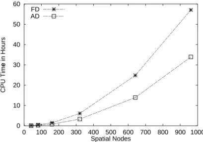
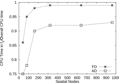
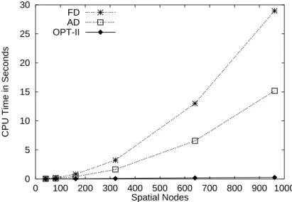
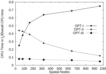
In the first section, the performance of a standard version ofDAESOLto handle also large scale problems as they arise from discretized PDEs is investigated for both the finite difference mode(FD)and the automatic differentiation mode(AD). In the latter mode the derivatives of the right hand side with respect to the states^u and the parameters^v are provided by the automatic differentiation toolADIFOR(Bischof et al., 1992 [15], 1994 [16], 1998 [17]). Analysis of the performance reveals that the computational effort for parameter estimation is mainly dominated by the frequent computation of^xw whose computational complexity increases quadratically with the number of spatial nodes^y

>. #

w C

.

In Section 3.2, we first outline an approach that circumvents the computation of^+w in each BDF step by using a modified Newton method (Dieses et al., 1999 [41]; Bock et al., 1995 [23]). The idea is to reduce the number of

+w

-computations by substituting them by directional derivatives of type^+w ⁴ .

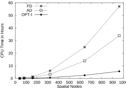
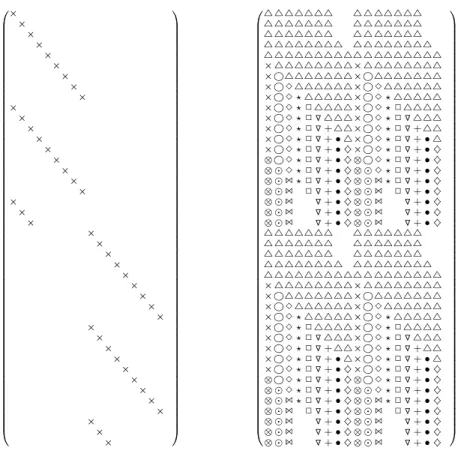
Secondly, in Section 3.3, we present an approach that removes the complexity order^y

>. #

w C

in order to further speed up the code. We exploit the fact that due to the use of fixed spatial grids the sparsity pattern induced by the spatial discretization of the PDEs remains unchanged in the course the reduced Generalized Gauss-Newton method. By identifying structural orthogonal columns of^xw (Curtis et al., 1974 [34]),^xw is computed via a compressed matrix requiring only

z|{

. w

instead of^. ^w directional derivatives. Thus, the computation of^+w is only dependent on the order of the spatial discretization routine and the number of PDEs and is independent of the number of spatial nodes. By this strategy, we manage to reduce the computation complexity of

xw

to the same complexity order^y

>. wFC

as the evaluation of the right hand side

.

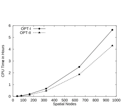
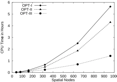
Combing both strategies, the modified Newton method and the compressed approach for the computation of

+w

, finally a speed up by a factor of 40 is gained for a parameter estimation problem with 2 PDEs and 961 spatial nodes. The CPU time is reduced from originally 2.5 days to less than 1.5 hours.

ECOPLAN:An approach for optimizing experimental conditions and sampling schemes (Chapter 4)

Due to the numerous problems encountered by estimating unknown parameters from water and solute transport processes, many researchers have claimed the need for methods to optimize experimental designs.

In order to address this problem, it has become popular among the soil science community within recent years to derive improved designs by analyzing two-dimensional response surfaces

(19)

Introduction 7

or by calculating sensitivity coefficients from hypothetical data. However, in both cases this is done on a tedious and cumbersome trial-and-error basis, rather than embedding the problem into the framework of optimization. There are only few studies that consider this problem in the context of optimal experimental design theory using statistical design criteria. The basis for this is the variance-covariance matrix, which describes the statistical quality of the parameter estimates. The objective of optimal experimental design is to minimize a function ^} of the variance-covariance matrix of the underlying parameter estimation problem. Often one of the classical designs, ^G -, ^~ -, or -optimality are used, which aim at minimizing the determinant, the trace, and the largest eigenvalue of the variance-covariance matrix, respectively. So far this approach has only been used to derive optimal sampling schemes, i.e. optimal allocations of measurement points in time and space.

However, considering in particular column or mini-lysimeter studies, there are by far more possibilities to influence the experiments in order to obtain good measurement data with respect to parameter estimation. In this work, for the first time an approach is presented that enables to optimize both

t the experimental conditions, e.g. initial soil profiles, irrigation and application schemes, and

t the sampling design

with respect to parameter estimation in transport and degradation processes of xenobiotics in soils. The approach presented follows the concepts worked out within the BMBF project “Op- timale Versuchsplanung f¨ur nichtlineare Prozesse” (FKZ: 03 D 0043, principal investigators:

Bock, Schl¨oder). Within this project the optimal experimental toolVPLANfor parameter estimation problems constrained by ODEs and DAEs was developed (Bauer et al., 1999 [9]; K¨orkel et al., 1999 [83]; Bauer et al., 2000 [10]). On the basis ofVPLANand the parameter estimation toolECOFIT, the new toolECOPLANthat is suitable for optimal experimental design in water and reactive solute transport processes has been developed.

In Section 4.1, the optimal experimental design problem is formulated as an optimal control problem. Hereby, in addition to time-independent control variables and time-dependent control functions, binary weights for feasible measurement points in time and space are considered. For the numerical solution, as described in Section 4.2, a direct approach is employed where time- dependent control functions and state constraints are discretized on a suitable grid. This results in a finite dimensional, nonlinear constrained optimization problem that is solved by a struc- tured SQP-method. In Section 4.3, we discuss practical requirements for optimal experimental designs and possible extensions, such as sequential designs or designs for model discrimination.

Application ofECOFITandECOPLANto column, lysimeter and field studies (Chapter 5) As this is an interdisciplinary work, the application of the developed toolsECOFITandECO- PLANto column, lysimeter and field experiments is of particular interest. Different types of examples are presented, some of them using hypothetical data, some of them building on data that

(20)

is provided by experiments. In the first two examples, in order to enable a controlled scenario, measurement data is generated by solving the forward problem for a predefined true parameter set followed by adding pseudo-normally distributed noise. In the first example, Section 5.1, the performance ofECOFITis investigated for identifying water and solute transport parameters from different noisy data sets starting from poor initial guesses. The second example, Section 5.2, is devoted to the treatment of parameter estimation problems in layered soils.

In Section 5.3, we also study a field experiment even though the main focus of this work is upon inverse modeling in column and mini-lysimeter experiments. Here,ECOFITis used for estimating the van Genuchten parameters^. ,^e and^T ^* from field data. The experimental part of this study was carried out by Aden (1999 [3]; [2]) at a BASF test site in the upper Rhine valley.

Time domain reflectrometry (TDR) was employed to monitor the volumetric water contents in several depths. For this type of experiments, an adequate model is developed.

In two cases ECOFIT is applied to mini-lysimeter studies as they are performed for registration purposes. In the first case, Section 5.4, the transport and sorption behavior of three European soils are determined. The experiments were carried out by the Staatliche Lehr- und Forschungsanstalt (SLFA), Neustadt/Weinstr. (Fent, 1999 [50]). After the application of the non-reactive tracer bromide and of a

)Y

-labeled test substance X, the undisturbed soil cores were irrigated by a constant daily rate and leachate volumes were sampled. A model is worked out for this typical class of outflow experiments and the unknown transport and sorption parameters are estimated.

In a second study, Section 5.5, we investigate the environmental fate of the grass herbicide S-Metolachlor and its two main metabolites by means ofECOFIT. The data used for inverse modeling was obtained by mini-lysimeter experiments performed by Horn (1999 [62]) at a Novartis test site in Switzerland. In this study the mini-lysimeters were exposed to normal climatic conditions. Again, the unknown parameters, such as the linear sorption coefficients and the degradation rates, are determined based on leachate data. This parameter estimation problem, however, suffers from the problem of ill-posedness due to the insufficient information provided by the available data.

In the last section, the potential and the features ofECOPLANare demonstrated on a hypothetical column outflow experiment where both water and solute transport parameters are estimated simultaneously. In a first scenario, the impact of optimized experimental (boundary) conditions, such as irrigation scheme and substance concentration in the irrigation water, is studied for a given sampling scheme. The objective of a second scenario is the simultaneous optimization of both the sampling scheme and the experimental conditions. Comparing intu- itive designs with the experimental design optimized byECOPLANreveals the huge potential of optimal experimental design. With the same number of observations parameter variances can be drastically reduced. Moreover, questions about the influence of neglecting or adding certain types of data on the quality of parameter estimates can be easily answered. We can, for example, decide a priori, whether profile concentrations obtained by slicing soil columns at the end of an experiment can essentially improve estimation results or not. Several examples are presented and discussed in detail.

(21)

Introduction 9

All computational results presented in this work were obtained on a workstation SUN ULTRA SPARC 10 (300MHz) running Solaris version 7.

(22)

(23)

Chapter 1 Mathematical Problems in the Environmental Fate Modeling of Xenobiotics

Registration of xenobiotics requires, besides the ecotoxicological risk assessment, studies about the environmental fate of the employed substances. On the one hand, regulatory authorities are interested in parameter values such as sorption coefficients, e.g.^TWN -values, or degradation rates.

On the other hand, more recently simulation results have to be submitted as well. A European consensus about a simulation model has not been obtained yet. In most Western European countries the one-dimensional models PELMO (Klein, 1995 [72]; Jene, 1998 [69]), PEARL (Tiktak et al., 1999 [125]), PRZM (Carsel et al., 1998 [29]) or MACRO (Jarvis and Larsson, 1998 [68]) are used.

As the tools developed in this work should also be applicable to registration studies, the choice of the model equations considered is based on the simulation models used in current practice by industry and regulatory authorities.

In the first two sections the relevant model equations applied for registration calculations, i.e. the Richards equation for the water transport, the convection-dispersion equation for the solute transport, linear sorption and degradation, are presented. In addition, more recent model approaches for nonlinear processes such as Langmuir sorption or Michaelis-Menten kinetics are discussed. These more complex models are generally not available in commonly used simulation tools. Up till now, nonlinear approaches of this type are of minor interest, as the risk assessment of xenobiotics required by authorities is mainly constrained to linear approaches.

In Section 1.3 special aspects associated with the modeling of column, lysimeter and field experiments, in particular the adequate description of upper and lower boundary conditions are addressed. The following section is devoted to the formulation of the parameter estimation problem as it typically arises in the environmental fate studies. An overview of parameter estimation tools used in current practice is given. Frequently encountered pitfalls and shortcomings are summarized and the need for more sophisticated methods is motivated. In Section 1.5 an optimal control problem is derived for the determination of optimal experimental conditions and

11

(24)

sampling schemes for column and mini-lysimeter studies with respect to parameter estimation.

Strategies employed in practice to treat the design problem are reviewed.

1.1 Transient Flow of Water in the Unsaturated Soil

Under natural conditions, as they arise in lysimeter or field experiments, water flow through soil is in general instationary, i.e. it varies in time and space. In the following the Richards equation for water transport in the unsaturated zone is derived. Frequently used parameterization of the soil water characteristic and the unsaturated hydraulic conductivity are presented which are assumed to hold for soils with uni-modal pore size distributions.

However, in the case of macroscopic structures like fractures or macropores more compli- cated models, e.g. two domain approaches considering macropore flow (Jarvis, 1991 [67]) or capillary flow (e.g. Diekkr¨uger, 1992 [36]; Richter et al., 1996 [104]) should be employed. Even though these approaches are not discussed in the following, they can, in principle, be treated by the methods developed in this work.

1.1.1 Richards Equation

The transport equation for water in a variably saturated rigid porous medium can be derived by the mass conservation equation, which in the one-dimensional case is of the form

E

1 5X

/

;

a

(1.1) where^E

is the volumetric water content,^/

( $)

is the volumetric water flux density, S

(

$)

is a source/sink term,^;

0

is the vertical coordinate (positive downward), and¹

(2

is time.

We assume Darcy’s law

/5

T @ O

;

(1.2) to hold, which relates the water flux^/ with a hydraulic gradient by the hydraulic conductivity

T

$) (2

. However, in contrast to the case of saturated conditions, the hydraulic conductivity is a function,

T >EFC

$) (2

, that not only depends on the geometry of the pore space and the physical properties of the water phase but also on the geometry of the water phase.

The soil water potential

@ O

$)

(

$#

is composed of several partial potentials, i.e. the gravitational potential^@ ^S

$) ( $#

, the osmotic potential^@ ^*

$) ( $#

and the tensiometer potential^@Uoqp

$) ( $#

:

@ O 5 @ S @ *

@Uoqp

(1.3) The gravitational potential

@ S

5X7:9

>

;V;

H C

(1.4)

(25)

1.1 Transient Flow of Water 13

describes the energy that is necessary to move water from a reference level ^; ^H to a depth ^; , where^7:9

is the mass density of water and is the acceleration of gravity

|"! $#

. In the following we neglect the osmotic potential^@ ^* and assume the air pressure to be constant.

Considering only one component of the tensiometer pressure

@Uoqp

, namely the matric potential

@BA

$) ( $#

, (1.3) reduces to

@ O 5 @ S

@BA

5

@UA

4 >

;D;

H C

(1.5)

with^457:9

"!F$#

. The matric potential^@UA is the energy that is required to move water into the porous medium.

Combining the mass conservation equation (1.1) with the Darcy law (1.2) and putting the reference level^; ^H ⁵ we get the Richards equation

E

1 5

;

T

>-E C

;

@BA

4;

a

(1.6) Treating

E

as a function of

@UA

, as outlined in detail in the next section, we can apply the chain rule to

E\ 1

and rewrite

T

as a function of

@BA

,^T

>q@UAVC

X$)0(2

. Thus, we end up with the Richards equation in the matric potential form

=>q@UAC

@UA

1 5

; T

>@BADC

;

@BA

4;

a

(1.7) where

=>q@UAVC

5

E

@UA

$) 0( #

is the specific soil water capacity. Note, that (1.7) is valid for both the saturated and the unsaturated case.

On the other hand, we can also interpret

@UA

as a function of

E

. By applying the chain rule to

@UAD ;

, we obtain the Richards equation in the water content form

E

1 5

;

G

>E C

E

;

4

T

>E C

a

(1.8) where

G

>-E CP

5

T

>EFC

=?>E C

=?>EFC

5

@UA

E (1.9)

is the soil water diffusivity

# ( $)

.

a 5

a >E C ( $)

denotes the source/sink term in

E

in contrast to

a 5 a >q@UAC

. Due to the fact that

=?>E CP

$) ( $#

as the soil becomes saturated, (1.8) is only defined for the unsaturated case. Note, that (1.8) can be formally interpreted as a convection-dispersion equation, where formally ^b

>-E C

5

4 >

T

EC

denotes the convection velocity and

G

>EFC

the dispersion coefficient (Roth, 1996 [106]).

1.1.2 Parameterization of Hydraulic Functions

Several parameterizations of the unsaturated soil hydraulic properties, i.e. the soil water characteristic and the unsaturated hydraulic conductivity are known. In order to enable a compact formulation we introduce the normalized water content

k

s 5 E E

E * E

(1.10)

(26)

where

E *

is the saturated volumetric water content and

E

is the residual volumetric water content.

One of the first models was given by Brook and Corey (1964 [27]) and Burdine (1953 [28]):

s>q@UAC

5

:

¢¡

@UA¤£¥@Un

¢¡

@UA¤¦8@Bn (1.11)

T

>@UAVC

5 T * s

+§¨#©

(1.12) where

@Un $)( $#

denotes the bubbling pressure, ^j

k

the pore size distribution index, and

T *

$) (2

the saturated hydraulic conductivity.

Basing on (1.11) van Genuchten (1980 [129]) developed a class of functions that is contin- uously differentiable and applicable to a broader range of soil types:

s?>q@UAVC

5 >

e2ª

@UA

ª

C«

A

¢¡

@UA¤£

¢¡

@UA¤¦

(1.13)

where

k

, ^.

k

and ^e

$) 0( #

are positive fitting parameters. In connection with the statistical pore size distribution model of Mualem (1976 [94]) for the unsaturated hydraulic conductivity

T

>@BADC

5 T * > >

e2ª

@UA

ªC « $) > >

e¬ª

@BA

ªC « C A C #

> >

e¬ª

@BA

ªC « C

(1.14) frequently

5 .

is used.

Conversely, both functions can be also expressed as functions of

E

:

ª

@UA,>EFC

ª5 e

$)

s

,®

®

¯

\¡

@UA°£

(1.15)

T >-E C

5 T * s ®

s ®

A #

(1.16) Remark 1.1 (Hysteresis)

The parameterization for the soil water characteristic mentioned above does not consider hysteresis. For models that include hysteresis see for example (Kool et Parker, 1987 [78]). It should be noted that the hydraulic conductivity in

@BA

generally shows a strong hysteresis while hysteretic effects for the formulation in^E are often negligible.

1.2 Solute Transport through the Subsurface with Transient Flow of Water

The processes associated with the environmental fate of xenobiotics in soils are very complex and by far not completely understood. Their adequate modeling, in particular for heterogeneous structures, is subject of current research.

(27)

1.2 Solute Transport through the Subsurface 15

In this section, we derive the convection-dispersion equation which is assumed to hold for the description of the transport of dissolved substances on the column and mini-lysimeter scale.

Under unsaturated conditions the convection-dispersion equation has to be solved together with the Richards equation. Several approaches for the modeling of linear and nonlinear sorption and degradation processes are presented.

1.2.1 Convection-Dispersion Equation

The transport of dissolved chemicals, e.g. xenobiotics, in a porous medium such as soil is driven by convection, molecular diffusion and dispersion. Considering also mass conservation for these processes the convection-dispersion equation for solute transport in the unsaturated zone can be derived.

Starting from the general continuity equation mass conservation of the total concentration

in the one-dimensional case requires

1 5

R

;±

`W

(1.17) where ^R

$#²(,$)-

denotes the total mass flux and

`

(,$)-

is a source or sink term representing the creation or disappearance of substance.

The total concentration can be decomposed into the respective concentrations occurring in the liquid, solid and gaseous phase:

³5

E 7 ! i

(1.18) where

is the concentration in the liquid phase,

!,

$)

is the concentration in the solid phase,⁷

is the bulk density,

is the concentration in the gaseous phase, andⁱ

is the volumetric air content.

For the total mass flux^R several components can be distinguished, namely molecular diffusion in the liquid and gaseous phase, dispersion, and convective transport along with the water flow. Each of these terms will be discussed in the following and model approaches will be given.

Molecular diffusion in the liquid phase

Molecular diffusion of dissolved substances in the liquid phase is caused by Brownian motion and leads to mixing due to concentration gradients. It is described by Fick’s law

R N

5X

GKN >-E C

;

(1.19) where^G´N

# (

$)

is called the coefficient of molecular diffusion. However,^GKN is not a constant but a function of^E and parameterizes the geometry of the water phase:

GKN >EFC

5

GIH

r

>-E C

(1.20)

(28)

where ^GIH

# ( $)

is the coefficient of molecular diffusion in pure water, and^r

>EFC k

is the tortuosity factor. This empirical tortuosity factor ^r ^{>-E C} is a function of the volumetric water content^E and takes into account longer flow paths due to the space geometry.

Often used approximations are based on the Millington-Quirk models for gaseous diffusion (Millington and Quirk, 1961 [91]), such as

r

>-E C

5 E ) H

©

l # (1.21)

or as proposed by Jin and Jury (1996 [70])

r

>-E C

5 E #

l #©

(1.22) Here

l

denotes the porosity of the soil. Kemper and van Schaik (1966 [71]) suggested the empirical parameterization

r

>-E C

5Xµm¶·¹¸

>-ºYE C

(1.23) where^µ

²

and

º k

are positive constants.

Molecular diffusion in the gaseous phase

According to Fick’s law the mass flux of substance in the gaseous phase

R\S

$# ( $)

due to molecular diffusion is given by

R\S

5

G *

;

(1.24) where^G ^*

P#(,$)-

is the coefficient of molecular diffusion in the gaseous phase. Employing the approach of Millington and Quirk (1961 [91]) we get

G * 5 i ) H

©

l # GKJdL

(1.25) with the coefficient of molecular diffusion in the air^GKJdL

# (

$)

. Dispersion

Superimposed on the diffusive transport is the dispersive transport. Mechanical dispersion arises from inhomogeneity of the pore space and leads to mixing caused by random water movement:

R A

5X

E G A

;

(1.26)

(29)

1.2 Solute Transport through the Subsurface 17

where^G

A

# ( $)

is the coefficient of dispersion in the liquid phase. For the one-dimensional case it is often assumed that ^G ^A increases linearly with the pore water velocity ^3»5 ^ª/$ª^¢E

0(,$)

G A>

/ C 5egf

ª/¼ª

E

(1.27) The dispersion length^egf

0

is determined by the geometry of the transport volume.

Remark 1.2

For the saturated case, the transport volume equals the pore space and can thus be treated as a constant. Under unsaturated conditions, however, the geometry of the water phase varies. Thus,

ef relies on the volumetric water content^E which varies in time and space.

The molecular diffusion in the liquid phase (1.19) and the dispersion term (1.26) are both proportional to the gradient ^; and thus are often combined to the hydrodynamic dispersion term

GKO >E / C 5

G´N >-E C

E G AW>

/ C

(1.28) Convection

The convective flux

R &

$# ( $)

translates the dissolved substance along with the water flux

/ R &

5X/F

(1.29) As convection is often the dominant component in the transport the correct description of water transport is a prerequisite for a meaningful modeling of the solute transport.

Collecting (1.28), (1.24) and (1.29) the total solute flux is given by

R

½5X

E GKO

; G *

;

/

(1.30) By combining now the continuity equation (1.17) with the total solute flux (1.30) we obtain the convection-dispersion equation

M

1 5

1

>E