zur
Erlangung der Doktorw¨ urde der
Naturwissenschaftlich-Mathematischen Gesamtfakult¨ at
der
Ruprecht-Karls-Universit¨ at Heidelberg
vorgelegt von
Dipl.-Phys. Dagmar Sigrun Isert aus Waiblingen
Tag der m¨undlichen Pr¨ufung: 14. Februar 2001
Gutachter: Prof. Ph D Sandra P. Klevansky
Prof. Dr. Michael G. Schmidt
submitted to the
Combined Faculties for the Natural Sciences and for Mathematics of the Rupertus Carola University of
Heidelberg, Germany for the degree of Doctor of Natural Sciences
Transport Theory for scalar Quarks and Gluons
presented by
Diplom-Physicist Dagmar Sigrun Isert born in Waiblingen, Germany
Heidelberg, 14.02.2001
Referees: Prof. Ph D Sandra P. Klevansky
Prof. Dr. Michael G. Schmidt
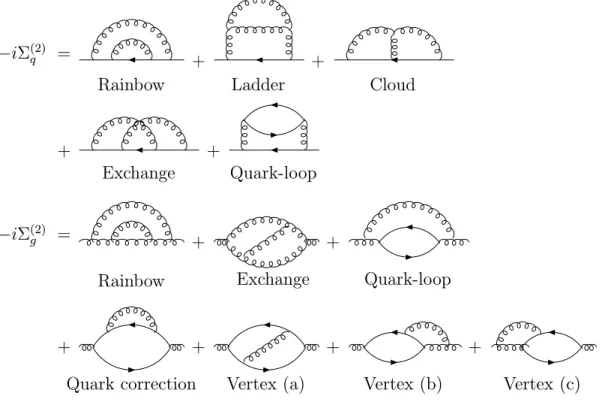
In dieser Arbeit werden die sogenannten Transport- und Constraintgleichungen f¨ur skalare Quarks und Gluonen aufgestellt. Es wird gezeigt, dass die Transportglei- chung ohne Ber¨ucksichtigung der Constraintgleichung in der Quasiteilchenn¨aherung zu einer Boltzmann-artigen Gleichung f¨uhrt. Die Analyse aller auftretenden Selbst- energiegraphen macht deutlich, welche Rolle sie spielen: Einige Graphen f¨uhren zu den erwarteten Wirkungsquerschnitten, w¨ahrend andere Graphen Feynman- Diagramme von Streuprozessen niedrigerer Ordnung renormieren.
Bei der Berechnung der Transportgleichung treten in einzelnen Selbstenergiegraphen sogenannte Pinch-Singularit¨aten auf. Durch eine explizite Rechnung kann gezeigt werden, dass sie sich im Gleichgewicht wegheben. F¨ur Systeme im Nicht- Gleichgewicht werden verschiedene Ans¨atze untersucht, die allerdings nicht zur Aufhebung aller Pinch-Singularit¨aten f¨uhren.
Bei Ber¨ucksichtigung der Constraintgleichung erhalten die Propagatoren eine endliche Breite, wodurch die Pinch-Singularit¨aten nicht mehr auftreten. Daf¨ur wird die Berechnung der Transportgleichung komplizierter, und sie kann nicht mehr in eine Boltzmann-artige Form gebracht werden.
Transport theory for scalar quarks and gluons
Abstract
In this work, we have detailed the calculations of the transport and constraint equa- tions for a theory of scalar quarks and gluons with self-interactions. Special care has been taken in particular in understanding how the transport equation, taken on its own, leads to a Boltzmann-like equation when considered in the quasiparticle ap- proximation. Through the analysis of all self-energy graphs that occur it is evident which role they play: certain graphs give rise to the expected cross sections, while others serve to renormalize diagrams of lower order scattering processes.
In the calculation of the transport equation, so-called pinch singularities arise in individual self-energy diagrams. We demonstrate explicitly how they cancel in equi- librium. For the case of non-equilibrium, several ans¨atze are investigated, but none of them leads to the cancellation of all pinch singularities.
Finally, the constraint equation is considered. This leads to the introduction of a finite width into the propagators. The main advantage of this is that no pinch singularities can possibly occur. The disadvantage, however, is that the calculations become very cumbersome and it is no longer straightforward to cast the transport equation into a form which can be recognized as being Boltzmann-like.
1 Introduction 3
2 Model of scalar quarks and gluons 9
2.1 Scalar partonic model . . . 9
2.2 Elastic qq scattering at high energies . . . 10
3 Field theory in and out of equilibrium 15 3.1 Finite-temperature field theory . . . 15
3.2 Transport theory . . . 22
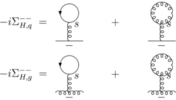
4 The collision integral - mean field self-energies 29 4.1 Hartree self-energies . . . 30
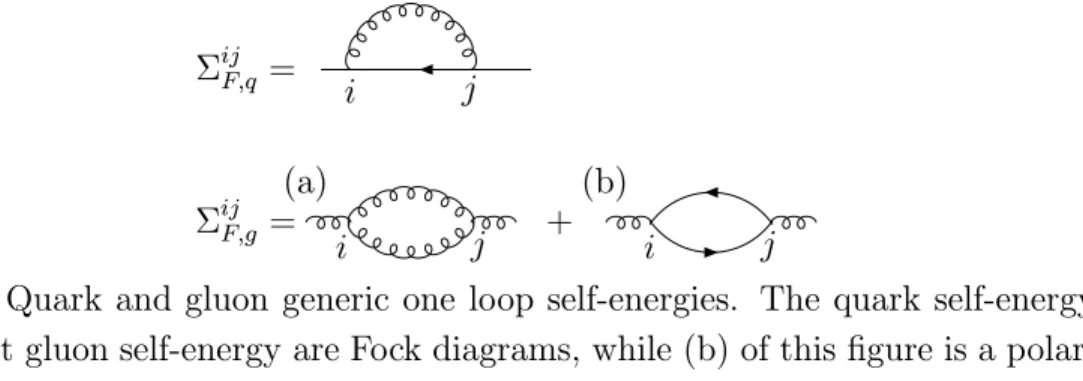
4.2 Fock self-energies . . . 31
5 The collision integral - two loop self-energies 35 5.1 2→2 scattering processes . . . 37
5.1.1 Quark-quark and quark-antiquark elastic scattering . . . 37
5.1.2 Scattering cross sections involving quarks and gluons . . . 40
5.2 Higher order corrections to the processqq¯→g . . . 44
6 Three and more loop self-energies 57
6.1 Three loop self-energies . . . 58
6.2 n to m processes . . . 61
7 Pinch singularities 63 7.1 Cancellation of pinch singularities in equilibrium . . . 64
7.1.1 Model with one type of particle . . . 64
7.1.2 Model with two particle types . . . 70
7.2 Pinch singularities in non-equilibrium . . . 72
8 The constraint equation 77
9 Summary and conclusions 81
A Wigner transforms 85
B Color factors 87
Introduction
In searching for the fundamental particles of matter, many new hadrons were found in accelerator experiments in the 1950/60’s. In order to organize this ‘hadron-zoo’, quarks were postulated as fundamental particles. Due to the Pauli-principle for quarks in hadrons, it was necessary to postulate a new quantum number called color which is the charge of the strong interaction. The number of colors (three) is confirmed by several experiments. Under normal conditions only color neutral objects (hadrons) are observed, i.e. three quark states (baryons) or quark-antiquark pairs (mesons). Nevertheless, one believes that this confinement falls away for matter under extreme conditions.
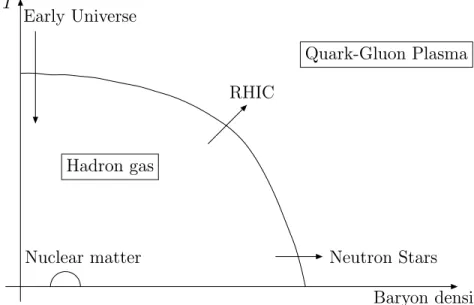
In the hadronic phase, confinement plays a dominant role and the chiral sym- metry is spontaneously broken. For sufficiently high temperatures and/or baryonic density a phase transition is believed to take place. The new phase is the so-called quark-gluon plasma (QGP); quarks and gluons are free particles that are deconfined and the chiral symmetry is restored. Note that it is often assumed that both phase transitions take place simultaneously, i.e. at the same temperature.
In a naive view, this phase transition is frequently given heuristically as shown in Fig. 1.1. There it is assumed that an equilibrium description is valid. It is believed that the early universe passed approximately 10µs after the big bang - when it was cool enough - through this phase transition. Obviously this was a unique ‘experiment’ and cannot be repeated. But in relativistic heavy ion collisions (RHIC) this phase transition should take place, too, since the conditions for the phase transition, extremely high energy densities, can be reached.
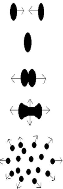
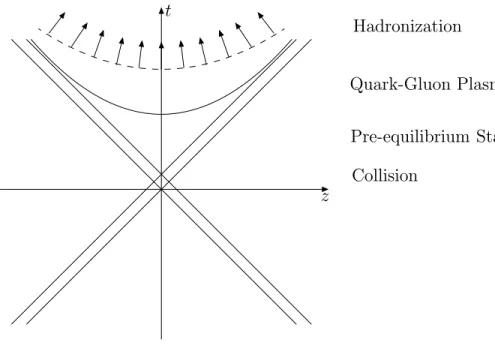
Thus let us review the scenario for an ultra-relativistic heavy ion collision which is shown schematically in Fig. 1.2. Its evolution in space-time is presented in Fig. 1.3.
For high beam-energies (ECM > 50GeV /nucleon), two Lorentz contracted nuclei pass through each other. Then, shortly after the collision, an energy density of
3
Baryon density ρ T
Quark-Gluon Plasma
Nuclear matter Hadron gas Early Universe
Neutron Stars RHIC
Figure 1.1: Phase diagram for hadronic matter.
one or two orders of magnitude greater than that of ground state nuclear matter (0.15GeV /f m3) is expected to be attained. At this stage, one assumes that the quarks and gluons are no longer confined and form a dense plasma. The excited partons interact with each other, and if the interactions occur frequently enough, the system reaches a local thermodynamic equilibrium, the quark-gluon plasma. Finally the partons hadronize, i.e. hadrons are formed and recede from the collision region.
Note that due to the fact that the collision takes place over an extremely small time scale, it is not clear that chemical and thermodynamical equilibrium are reached:
this underscores the cartoon like nature of Fig. 1.1.
Thus, in this thesis we address the question as to how the partons evolve after the collision to a point in which thermodynamic equilibrium is possibly reached.
This evolution is described by the evolution equations for the distribution function fa(x, p) in phase space wherefa(x, p)d3xd3pgives the probability of finding a parton of type a in d3x around ~x and with a momentum in d3p around ~p. Now ordinary zero temperature field theory is insufficient for a description of the evolution of the system. One cannot assume that the system passes through a series of equilibrium states, and therefore one needs a description in terms of non-equilibrium field theory.
Within this transport theory, the two evolution equations for the distribution func- tion fa(x, p), the so-called transport and constraint equations can be constructed.
The natural underlying Lagrangian for the description of heavy ion collisions is that of quantum chromodynamics (QCD). Studying this Lagrangian in the context
Figure 1.2: Schematic drawing of an heavy ion collision.
of non-equilibrium field theory introduces several difficulties in addition to simply the complexities that non-equilibrium theory gives rise to: these are gauge invari- ance, renormalization and the non-abelian like nature of the interaction. Clearly to develop a description which can simultaneously account for all these facets, an exact description of the transport equations with all of these facets is required. To the present date, however, each of these facets produces problems of their own. In addition, transport theory per se has only been worked out for few simple inter- acting systems often assuming contact and abelian interactions and also with the restriction of understanding only the lowest order processes. Consequently the ap- proaches in the literature address one or the other problem in some form. We list some approaches that attempt to develop the relevant equations for QCD:
• Many authors rely on an intuitive extrapolation of the semiclassical Boltzmann equation in their applications (see for example, Geiger and M¨uller [1, 2] who examine heavy ion collisions in extreme conditions). Here an educated guess at an extended Boltzmann equation is made in order to develop a numerical simulation algorithm. An assumption about which processes should be con- sidered in the collision integral is made on a purely heuristic basis. In such an approach, often the transport equation alone is examined; the constraint equation is simply neglected. In such studies a first attempt at putting this
z t
Collision
Pre-equilibrium Stage Quark-Gluon Plasma
Hadronization
Figure 1.3: Space-time diagram of the evolution of an heavy ion collision.
application on a firm theoretical basis was subsequently made by [3].
• Some authors have centered their investigations on a full quantum treatment of the non-equilibrium Green function equations (see for example [4, 5, 6]). This approach has an aesthetic appeal, but in practice, there is little possibility of its application, as the complexity of solving many (16 or more) coupled integro- differential equations can only be performed under severe physical restrictions, namely that of no collisions.
• Progress in understanding collision theory has been made with the recent de- velopments in real time Green function theory to calculate properties of sys- tems in equilibrium. A theoretical methodology for handling non-equilibrium Green functions was developed by Schwinger and Keldysh [7, 8]. Later, in the 1980’s, the development of thermal field theory was initiated by Umezawa [9]. The resulting matrix of real time Green functions has revealed a strik- ing resemblance to the matrix of Green functions that is obtained in the Schwinger-Keldysh formalism. One can in fact quantifiably demonstrate that Schwinger-Keldysh and real time thermal field theory yield the same results in the limit that one considers equilibrium systems. Both formalisms are un- wieldy, especially in contrast to the elegant formulation of equilibrium field theory by Matsubara, that was developed in the 60’s, and which simply makes
extensive use of function theory. The historically late development of real time Green function theory is due to the fact that several difficulties in this approach are immediately evident: Products of retarded and advanced Green functions occur, so that integration along the real axis becomes problematic as the infinitesimal element → 0: the contour is pinched and the function is singular. So called pinch singularities also manifest themselves as products of delta functions when working in a causal / acausal framework. The fact now that two completely different formulations of equilibrium field theory ex- ist has enabled one to understand these apparent difficulties in the real time approach, and this in turn enables one by comparison, to investigate similar situations in the non-equilibrium theory.
Our view in this work is directly to focus on the issue of constructing an exact transport theory in which non-abelian interactions occur and which pushes transport theory into the two-loop level and beyond in constructing an exact solution. In order to do this, the issue of gauge invariance is an unnecessary added degree of complexity, and we therefore do not investigate a gauge theory like QCD per se, but rather a simpler model of QCD which has the properties that it is scalar, and secondly, includes self-interactions in such a fashion that it describes pomeron behavior in elastic quark-quark scattering. The last feature of pomeron behavior is essential in some simulation models [10] that give good descriptions of experimental data for heavy ion collisions at energies attainable today. For the colliders RHIC and especially for LHC, it is unclear whether these pomeron based models will be able to account for the physics, necessitating a deeper understanding of the evolution of the constituents at a parton level.
Within our model of scalar quarks and gluons, we have been successful in building an appropriate transport theory and constructing a collision term exactly for two loop self-energies. This work goes beyond all previous analysis in that the complexity of the interaction introduces a plethora of terms (previously unknown), and the interpretation of which has been clarified. The results are generalized beyond the two loop level and a Boltzmann-like equation is obtained. Multiparticle production and annihilation processes associated with this interaction are seen to occur. Since the quasiparticle approximation is used, the issue of pinch singularities arises, so that it is necessary to check whether and how singular behavior is removed from the transport equations. For consistency, the constraint equation is also examined.
This thesis is structured as follows. In Chapter 2, we introduce our model for scalar quarks and gluons. Furthermore, we show how the pomeron like behavior emerges from elastic quark-quark scattering in the Regge limit. Since the study
of transport theory is similar to equilibrium real time field theory, it is useful to gain knowledge from comparison. Therefore Chapter 3 is devoted to the revision of finite-temperature field theory and the transport and constraint equations are constructed in transport theory. Then the collision term of the transport equation is evaluated for the mean field self-energies in Chapter 4 and for the two loop self- energies in Chapter 5. In Chapter 5, we will in addition address the question as to which propagators should be used for the evaluation of scattering amplitudes - non-equilibrium or T = 0 propagators. In Chapter 6, the contributions beyond two loop self-energies to the collision term are considered. We devote Chapter 7 to the cancellation of pinch singularities. First, we demonstrate explicitly their cancellation in equilibrium field theory for several cases. Then we tackle the question whether and how pinch singularities are canceled in non-equilibrium. In Chapter 8, the second evolution equation, the constraint equation, is taken into account.
Finally we conclude in Chapter 9. Wigner transforms are listed in Appendix A for completeness. Appendix B shows explicit calculations of color factors for two loop self-energies.
Model of scalar quarks and gluons
In this chapter, we introduce and discuss the scalar partonic model, and give the equations of motion for quark and gluon fields. We briefly review high energy scattering within this model.
2.1 Scalar partonic model
We study a partonic model of QCD inspired by Polkinghorne [11] and used by Forshaw and Ross [12] that contains scalar partons. Quarks and antiquarks are described by complex scalar fieldsφ, and gluons as the scalar fieldχcoupled through the Lagrangian
L = ∂µφ†i,l∂µφi,l+1
2∂µχa,r∂µχa,r− m2
2 χa,rχa,r
−gmφ†i,l(Ta)ji(Tr)ml φj,mχa,r− gm
3! fabcfrstχa,rχb,sχc,t. (2.1) The quark fields are regarded as massless, as one generally assumes for high energy processes, while the gluons are usually assigned a massma prioriin order to avoid infra-red divergences. There is an interaction between quarks and gluons as well as a cubic self-interaction between gluons. Since in QCD the quartic interaction between gluons leads in elastic qq scattering to terms which are sub-leading in ln s, such a quartic interaction among gluons is not included within this model.
One notes that both the quark and gluon fields carry two labels. Both of these refer to color groups. The fact that a direct product of two color groups is necessary can be seen on examining the three gluon vertex term. This term must be symmetric under the exchange of two gluons since they are bosons. In addition, one expects that the interaction vertex should be proportional to the (antisymmetric) structure
9
constants of the color group. A single color group cannot meet these requirements, and the simplest combination which can is a product of two SU(Nc) groups. Thus the gluon field carries two color indices (a, r = 1...(Nc2−1)). Since the quark field transforms in the fundamental representation of both of these SU(Nc) groups, it must carry two color indices as well (i, l= 1...Nc). The matrices Ta and Tr are the generators and fabc and frst are the structure constants for the two SU(Nc) groups respectively. Thus they satisfy
[Ta, Tb] =ifabcTc, [Tr, Ts] =ifrstTt. (2.2) Note in Eq.(2.1) that the flavor index of the quark fields is suppressed.
The equations of motion for the fields can be derived from the Euler-Lagrange equations. They are
2φ(†)i,l =−gm(Ta)ij(Tr)lmφ(†)j,mχa,r (2.3) for the (anti-)quarks and
(2+m2)χa,r =−gm[φ†i,l(Ta)ij(Tr)ml φj,m+fabcfrstχb,sχc,t] (2.4) for the gluons.
2.2 Elastic qq scattering at high energies
The main advantage of this simple partonic model is that a calculation of the elas- tic quark-quark scattering amplitude at high energies at T = 0 reflects pomeron behavior. In this section, we simply quote these results, and for details, we refer the reader to [12]. Note that these calculations are performed in equilibrium and at T = 0 in contrast to the rest of this thesis.
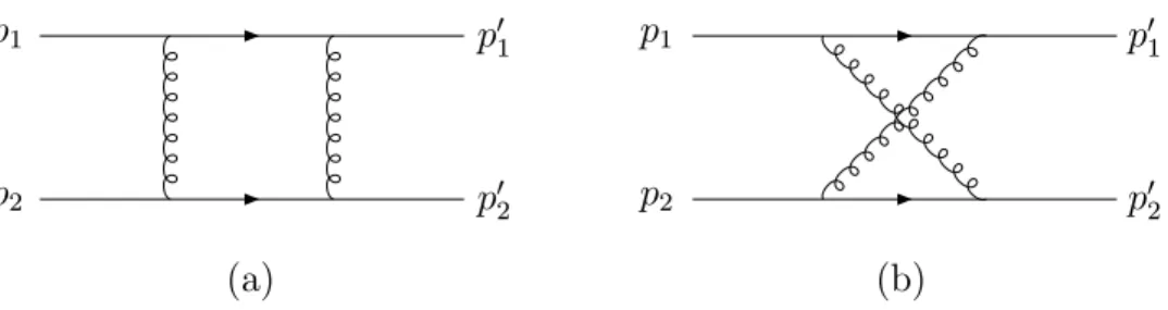
Quark-quark scattering is calculated via the exchange of a color singlet. It is assumed that the two quarks emerge from the scattering with the same color with which they entered and that they have different flavors. Therefore one has to con- sider only diagrams with at least two exchanged gluons, and one can neglect dia- grams with quarks that are exchanged in the t-channel. The incoming quarks have momenta p1 and p2, respectively. To lowest order, this process is shown in Fig. 2.1.
Denoting the transferred momentum as q=p1−p2, the Mandelstam variables read as s= (p1+p2)2 and t=q2. In the case of Fig. 2.1, it is easy to show that Fig. 2.1 (b) follows from Fig. 2.1 (a) only by a kinematical transformation, so that it is only
p2 p02
p1 p01
(a)
p2 p02
p1 p01
(b)
Figure 2.1: Leading order contribution to Pomeron exchange for elastic quark-quark scattering.
necessary to calculate graphs of type (a). The imaginary part of the amplitude can be identified according to the Cutkosky rules [13] to be
=A2.1(a)= 1 2
Z
d(P.S.2)A(g)0 (k)A(g)0 †(k−g), (2.5) where A(g)0 is the tree amplitude for single gluon exchange and reads as
A(g)0 (k) =−g2m2 1
(k2−m2) (2.6)
up to a color factor. R d(P.S.2) refers to the phase space of the two lines which are cut, i.e.
Z
d(P.S.2) =
Z d4l (2π)3
d4l0
(2π)3 δ(l2)δ(l02) (2π)4δ4(p1 +p2−l−l0). (2.7) One integration can be immediately performed, leaving one further integral over the momentum k of the exchanged gluon as
Z
d(P.S.2) = 1 (2π)2
Z
d4k δ((p1−k)2)δ((p2+k)2). (2.8) The further calculations are now performed in the center-of-mass frame in which the incoming quarks are considered to be along the z-axis, i.e.
p1/2 =
√s 2 ,±
√s 2 ,0
!
. (2.9)
Then it is useful to parametrize the integrated momenta k in terms of Sudakov parameters ρ and λ:
k =ρp1+λp2+k⊥= (ρ+λ)
√s
2 ,(ρ−λ)
√s 2 ,k
!
, (2.10)
where k⊥ is the momentum transverse top1 and p2 and this two-dimensional vector is represented by the boldface k. Then the phase space becomes
Z
d(P.S.2) = s 8π2
Z
dρ dλ d2kδ(−s(1−ρ)λ−k2)δ(s(1 +λ)ρ−k2) (2.11) where s = 2p1p2 was used. In the Regge limit s |t| the momentum transferred q is dominated by its transverse component, i.e.
t =q2 ≈ −q2. (2.12)
Similarly one finds
k2 ≈ −k2 (2.13)
and
(k−q)2 ≈ −(k−q)2. (2.14)
Performing the integration over ρ and λ, one finds for the imaginary part of the amplitude
=A2.1(a)= (Nc2−1)2 16Nc4
g4m4 16π2s
Z
d2k 1 k2+m2
1
(k−q)2+m2 (2.15) where the color factor has been included.
One expects now to obtain leading lns contributions for the scattering amplitude because the calculations are performed in the Regge limit. s/t is negative and therefore the relation
ln
s t
= ln s
|t|
!
−iπ (2.16)
holds. Since A2.1(a) has an imaginary part, its real part must have a logarithm with equal coefficient but opposite sign. The contribution of Fig. 2.1 (a) is thus proportional to
1
s ln s
|t|
!
−iπ
!
. (2.17)
In order to obtain the contribution from Fig. 2.1 (b) the Mandelstam variable s is replaced by u. Since u/t is positive, this diagram has no imaginary part. Therefore its contribution reads
1 uln
u t
. (2.18)
In the Regge limit u ≈ −s. Therefore the logarithms in A2.1 = A2.1(a) +A2.1(b)
cancel and we are left with the imaginary part of A2.1(a) given in Eq.(2.15).
The higher order calculations are tedious and we therefore state only the results.
p2 p02
p1 p01
Figure 2.2: One-rung ladder diagram.
The next-to-leading order contribution is given by the so-called one-rung ladder diagram shown in Fig. 2.2. Its contribution is of order g2lns relative to the leading contribution calculated above. The other three gluon diagrams like vertex correction diagrams or a digram with three exchanged gluons are subleading and therefore neglected.
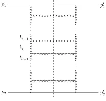
This result can be generalized. Thus the order (g2lns)ncorrection to the leading order contribution is given by the n-rung uncrossed ladder diagram, n = 1...∞, as shown in Fig. 2.3. The dashed line indicates the cut taken for the direct application
p2 p02
p1 p01
ki+1 ki
ki−1
Figure 2.3: n-rung ladder diagram with cut line (dashed line).
of the Cutkosky rules. Applying these rules and keeping only the leading lns con- tributions in evaluating the infinite sum of uncrossed ladder diagrams, one obtains
the following result for the imaginary part of the scattering amplitude
=A(s, t) = (Nc2 −1)2 16Nc4
g4m4 16π2s
Z
d2k 1
(k2+m2)((k−q)2+m2) s
|t|
!1+αP(t)
, (2.19) with the trajectory
αP(t)≈ −1 + g2Nc2 16π2
1 + t 6m2
. (2.20)
In the Regge limit, the real part of A(s, t) vanishes. Therefore A(s, t) is purely imaginary and given by Eq.(2.19).
We point out that the selection of ladder diagrams for the evaluation of the scattering amplitude, as indicated in Fig. 2.3 is highly suggestive, particularly with the cut drawn in. One might wish to conclude that (a) gluon production is dominant, and (b) that only ladder type graphs need be considered in constructing gluon emission / absorptive processes. As will be seen in transport theory, however, one finds that (a) is true, having its basis in the 1/Nc expansion, but (b) cannot be justified, as it depends on the special kinematical assumptions that are applicable to the quark-quark scattering amplitude, but which do not occur in the self-energy evaluation.
Field theory in and out of equilibrium
Since processes taking place in heavy ion collisions are most likely to occur out of equilibrium, this chapter is devoted to non-equilibrium field theory, namely to transport theory. As an introduction to and for comparison with non-equilibrium field theory, the first section describes finite-temperature field theory in equilibrium.
3.1 Finite-temperature field theory
In this section, we briefly review the basic ideas of quantum field theory at non-zero temperature in equilibrium (for more details see e.g. [14, 15, 16, 17, 18, 19, 20]).
There one can distinguish between two different approaches, the imaginary and the real time formalism (for a comparison of both see e.g. [21]). We will only mention the first one briefly and consider the second one in more detail. The imaginary time formalism was introduced by Matsubara. It provides an elegant and simple way of performing equilibrium calculations via integration in the complex plane.
Due to the formal similarities with zero temperature real time field theory, it is simple to identify the correct graphs. This means of calculation is widespread in the theoretical community due to its simplicity. By contrast, development of the real time formalism for finite temperature has been much slower. The reasons for this lie in the technical complexity and difficulties associated with real time formalism that have only recently been resolved or which are currently being addressed. Two famous candidates of the real time formalism are thermo field dynamics and the closed time path method. Especially the latter is important for us since it leads universally to all formalisms and in addition can be generalized to non-equilibrium
15
cases.
We start now with quantum mechanics: the probability amplitude F(q0, t0;q, t) of finding a particle at position q0 at time t0 when it was located at position q at time t is given by
F(q0, t0;q, t) =hq0e−iH(t0−t)qi. (3.1) Letting t→ −iτ, we find for the analytical continuation of F to imaginary time
F(q0,−iτ0;q,−iτ) =hq0e−H(τ0−τ)qi. (3.2) In a standard fashion the path integral representation is derived for F as
F(q0,−iτ0;q,−iτ) =
Z Dq(τ00) exp
(
−Z τ0
τ
dτ00
1
2mq˙2(τ00) +V(q(τ00))
)
(3.3) with q(τ) = q and q(τ0) = q0. Now we make the connection to quantum statistical mechanics: the partition function is defined as
Z(β) = Tre−βH =
Z
dqhqe−βHqi, (3.4) where β = 1/T is the inverse temperature. With the help of Eqs.(3.2) and (3.3), we can express the partition function in terms of a path integral as
Z(β) =
Z
dq F(q,−iβ;q,0)
=
Z
Dq(τ) exp
(
−Z β
0
dτ
1
2mq˙2(τ) +V(q(τ))
)
(3.5) with the boundary condition q(β) =q(0), i.e. over paths with periodβ in imaginary time. Now we turn to quantum field theory for a scalar field. The generating functional Z[β;J], with Z(β) =Z[β;J = 0], is then given as
Z[β;J] =
Z Dφexp
i
Z
C
dt [L(φ) +J(t)φ(t)]
, (3.6)
where we have assumed that the Lagrangian does not contain derivative interactions.
For simplicity, the spatial coordinates are suppressed in this section. The fields are subject to the (anti-)periodic boundary condition
φ(t−iβ) =η eβµφ(t), (3.7) with the chemical potential µand η=± for bosons and fermions respectively. The contour C must end at a point tf differentiating from the starting point ti by −iβ:
tf =ti−iβ. (3.8)
In addition to this requirement, the contourCmust have a monotonically decreasing imaginary part. The simplest choice for the contour would be a straight line along the imaginary axis fromti = 0 totf =−iβ. This so-called Matsubara contour leads to the imaginary-time formalism (ITF) which we will not consider here any further.
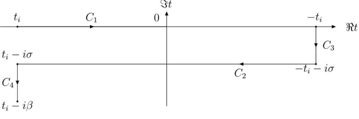
Other choices for the contour include the real axis and lead therefore to the real-time formalism. The standard contour is shown in Fig. 3.1. It goes fromti to −ti on the
<t
=t C1 0
ti −ti
C3
−ti−iσ C2
ti−iσ C4 ti−iβ
Figure 3.1: Real time contour
real axis, then drops vertically down to −ti−iσ, runs parallel to the real axis back toti−iσ and finally down toti−iβ. Here the parameterσ takes a value between 0 and β. One assumes that in the limitti → −∞the vertical segments of the contour C decouple in the path integral and do not contribute to Green functions with time arguments on the horizontal segments.
Writing the fields on the upper and the lower horizontal segments as functions of real times,φ−(t) =φ(t) andφ+(t) =φ(t−iσ), respectively, the generating functional for the Green functions reads as
Z[J−, J+] =Z[0,0]hTCexp
i
Z ∞
−∞dt φsJs
i, (3.9)
where the sign index s runs over {−,+} and J−(t) is defined to be the source on the upper segment and J+(t) = −J(t − iσ) the source on the lower one. The minus sign in the latter absorbs the minus sign from the opposite direction of the lower contour. Note, that in our notation the ‘-’ sign is associated with the upper branch as in [23] and in contrast to [16]. In the 80’s, the ‘-’ fields were termed physical fields according to the idea that physical observables would be expressible in terms of Green functions with only ‘-’ fields on the external legs. The ‘+’ fields were consistently called ghost fields. This is not a valid supposition. As a simple example, the mass term ΠR is made up of both Π−− and Π−+, see Eq.(3.45). There are also other interesting physical quantities with ‘+’ fields on their external legs, see e.g. the collision term of Eq.(3.58).
Differentiation with respect to J−(t) and J+(t) then gives the real-time Green functions
Gsσ1...sN(t1, ...tN) := δiJs
1(t1)...δiJsN(tN)Z[J−, J+] Z[J−, J+]
J−=0,J+=0
. (3.10)
The contour ordering TC implies that this real-time Green function is the thermal average of a product of field operators where the ordering is such that the ‘-’ fields are time-ordered and put on the right hand side and the ‘+’ fields are anti-time-ordered and put on the left hand side. Performing a Fourier transform
Gsσ1...sN(ω1, ..., ωN) :=
Z
dt1...dtN exp
(
iX
i
ωiti
)
Gσs1...sN(t1, ..., tN) (3.11) yields the relation between Green functions with different values of σ,
Gsσ1...sN(ω1, ..., ωN) = exp
− X
i|si=+
σ ωi
Gsσ=01...sN(ω1, ..., ωN). (3.12) Note that the value σ = 0 corresponds to a closed time path (CTP) or Schwinger- Keldysh formalism, see Fig. 3.2, whileσ =β/2 corresponds to the choice for Thermo Field Dynamics.
t
−
+
Figure 3.2: Closed time path
There are two important relations which connect the Green functions for a given σ. The first one is the so-calledlargest-time relation. For its derivation we setσ = 0.
Let the time tj be the largest one, i.e. tj > ti, i = 1, ..., j−1, j+ 1, ...N. Then we find
Gsσ=01...−...sN(t1, ..., tj, ...tN)−Gsσ=01...+...sN(t1, ..., tj, ...tN)
= sgnPnhT˜(φ+...φ+) [φ(tj)T(φ−...φ−)]i − hhT˜(φ+...φ+)φ(tj)iT(φ−...φ−)io
= 0. (3.13)
Here sgnP gives the sign associated with the permutation that is needed to put the fields in the right order. So far, the si for i 6= j were arbitrary. Therefore we can
sum over all possibilities for the si’s with appropriate sign factors to get
X
s1,...,sN
(−1)#(i|si=+)Gsσ=01...sN(t1, ..., tN) = 0, (3.14) where #(i|si = +) denotes the number of indices i for which si = +. This is the largest-time equation although the special role of the largest time tj is not manifest any more. Fourier transformation and Eq.(3.12) gives a similar relation for arbitrary σ
X
s1,...,sN
(−1)#(i|si=+) exp
X
i|si=+
σ ωi
Gsσ1...sN(ω1, ..., ωN) = 0. (3.15) It is important to notice that the largest time equation holds true in non-equilibrium situations as well.
Now, the second important relation is the Kubo-Martin-Schwinger (KMS) rela- tion. It is only valid in equilibrium. For its derivation, we consider an alternative contour ˜C which can be obtained form the original one C of Fig. 3.1 with σ= 0 by flipping it about the =t-axis. This contour gives rise to different Green functions which satisfy a smallest time equation. These Green functions can be related to the original ones. Fourier transformation and the use of Eq.(3.12) then yields the KMS relation
X
s1,...,sN
(−1)#(i|si=+) Y
i|si=+
ηi exp
X
i|si=+
−xi+σωi
Gsσ1...sN(ω1, ..., ωN) = 0, (3.16) where xi =β(ωi−µi).
Finally, we state a complex conjugation relation for real-time Green functions [Gsσ1...sN(ω1, ..., ωN)]∗ =G¯sσ1...¯sN(ω1, ..., ωN) Y
si=+
ηiexi−2σωi, (3.17) with the conjugate index ¯si= +,−if si =−,+.
Since we are ultimately interested in propagators, we consider now the case N = 2. The largest-time equation (3.14) then reads
Dσ=0−− +Dσ=0++ =Dσ=0−+ +D+σ=0−. (3.18) Taking into account momentum conservation (ω1+ω2 = 0) and charge conservation (µ1+µ2 = 0), the KMS relation (3.16) gives
D−−σ=0+D++σ=0 =η ex1Dσ=0−+ +η e−x1Dσ=0+−. (3.19) Subtracting these two equations yields the usual form of the KMS relation for 2-point functions,
Dσ=0−+ =η e−x1D+σ=0−. (3.20)
From Eq.(3.10) one obtains the real-time propagators as iD−−σ (t−t0) = hT φ(t)φ(t0)i
iD++σ (t−t0) = hT φ(t˜ −iσ)φ(t0−iσ)i iD−σ+(t−t0) = ηhφ(t0−iσ)φ(t)i
iD+σ−(t−t0) = hφ(t−iσ)φ(t0)i. (3.21) These four propagators can be written in a compact matrix form as
Dσ = Dσ−− Dσ−+ Dσ+− Dσ++
!
. (3.22)
Then performing a Fourier transform yields Dσ(ω) = DF(ω) 0
0 −D∗F(ω)
!
+ [DF(ω)−DF∗(ω)] ηn(|ω|) eσω[Θ(−ω) +ηn(|ω|)]
e−σω[Θ(ω) +ηn(|ω|)] ηn(|ω|)
!
,(3.23) whereiDF is the zero-temperature Feynman propagator andn(ω) is the distribution function defined by
n(ω) = 1
eβ(ω−µ)−η. (3.24)
One popular choice is σ =β/2; then the matrix of propagators reads as
Dσ=β/2(ω) = DF(ω) 0
0 −DF∗(ω)
!
+ [DF(ω)−DF∗(ω)]
ηn(|ω|) eβµ2
q
n(|ω|)
q
1 +ηn(|ω|)[ηΘ(ω) + Θ(−ω)]
e−βµ2
q
n(|ω|)
q
1 +ηn(|ω|)[Θ(ω) +ηΘ(−ω)] ηn(|ω|)
!
, (3.25) where the identity
eβ(ω−µ)/2 = Θ(ω)
vu
ut1 +ηn(|ω|)
n(|ω|) + Θ(−ω)
vu
ut ηn(|ω|)
1 +n(|ω|) (3.26) was used. For later use, we give the explicit form of the propagators for bosons (η = +1) with vanishing chemical potential (µ= 0). With the Feynman propagator for a scalar particle,
iDF(ω) = i
ω2−E2+i, (3.27)
and the relation
±i
ω2−E2 ±i = P ±i
ω2−E2 +πδ(ω2−E2), (3.28) where P denotes the principal value, we find
iDF(ω)−iDF∗(ω) = 2πδ(ω2−E2) = π
E [δ(ω−E) +δ(ω+E)]. (3.29) This gives for σ =β/2
iDσ=β/2(ω) =
i
ω2−E2+i 0 0 ω2−−Ei2−i
!
+2πδ(ω2−E2) eβ|ω|−1
1 eβ|ω|/2 eβ|ω|/2 1
!
. (3.30) Another popular choice is σ = 0. For scalar particles with vanishing chemical potential the matrix of propagators reads as
iDσ=0(ω) =
i
ω2−E2+i 0 0 ω2−−Ei2−i
!
+ 2πδ(ω2−E2)n(|ω|) Eπ [δ(E−ω)n(|ω|) +δ(E+ω)(1 +n(|ω|))]
π
E[δ(E−ω)n(|ω|) +δ(E+ω)(1 +n(|ω|))] 2πδ(p2−m2)n(|ω|)
!
. (3.31) The four propagators are not independent, since they fulfill Eqs.(3.18) and (3.20).
Therefore it is possible to transform the matrix such that at least one component is vanishing. For a review of possible transformations see e.g. Ref. [22].
We now return to the general expression of Dσ(ω) in Eq.(3.23). In the vacuum limitµ→0 andβ → ∞, the usual zero-temperature field theory should be regained.
In this limit, the distribution function n(|ω|) vanishes and we are left with iDσ(ω) = iDF(ω) 0
0 iDF∗(ω)
!
+ [DF(ω)−D∗F(ω)] 0 eσωΘ(−ω) e−σωΘ(ω) 0
!
.(3.32) In addition to this we perform the limitσ → ∞which is e.g. for the choiceσ =β/2 automatically fulfilled. This gives
iD∞(ω) = iDF(ω) 0 0 iD∗F(ω)
!
, (3.33)
i.e. one has two identical decoupled copies of zero-temperature field theory as ex- pected.
The real-time Feynman rules are much the same as in zero-temperature field theory. The only difference is that a sign factor s = −,+ is assigned to each
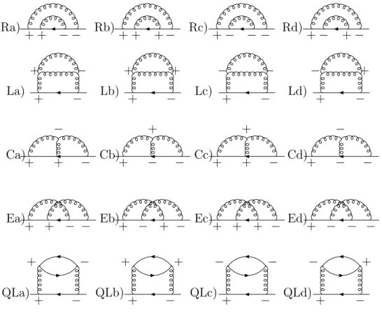
vertex. For Green functions and self-energies, the external vertices are fixed, and all internal vertices are summed over (which multiplies the number of graphs, see e.g. Fig. 5.2). A vertex with s = − corresponds to a factor −igm while a vertex with s = + corresponds to a factor +igm. (In order to introduce a dimensionless coupling constant g, a mass m is factored out.) A line connecting a vertex s with a vertex s0 corresponds to a propagator Dssσ0 given in Eq.(3.21).
An example of a scattering amplitude is shown in Fig. 5.5. The external vertices are fixed to be s =− while the internal vertices can be either ‘-’ or ‘+’ and one has to draw all possibilities. The complex conjugate of such an amplitude (in position space) is obtained by interchanging all ‘-’ vertices with ‘+’ vertices and vice versa in the original amplitude.
The CTP formalism corresponding to the choice σ= 0 is now easily generalized for non-equilibrium processes. This is the subject of the next section.
3.2 Transport theory
In this section, we briefly introduce the Schwinger-Keldysh formalism and the quasi- particle approximation. For the purpose of establishing our notation, we give the basic definitions and refer the reader to standard texts [23, 24, 25]. Then we derive the so-called transport and constraint equations following the lines of [26, 27, 28, 4].
While the last section was quite general, we refer in this section only to the cases that are relevant for us, i.e. for scalar quarks and scalar gluons (η = +1 andµ= 0).
The quark Green functions in the Schwinger-Keldysh formalism [7, 8] are defined through their average over operator products,
iSc(x, y) = DT φi,l(x)φ†j,m(y)E−Dφi,l(x)E Dφ†j,m(y)E =iS−−(x, y) iSa(x, y) = DT φ˜ i,l(x)φ†j,m(y)E−Dφi,l(x)E Dφ†j,m(y)E =iS++(x, y) iS>(x, y) = Dφi,l(x)φ†j,m(y)E−Dφi,l(x)E Dφ†j,m(y)E =iS+−(x, y)
iS<(x, y) = Dφ†j,m(y)φi,l(x)E−Dφi,l(x)E Dφ†j,m(y)E =iS−+(x, y) (3.34) and for the gluons as
iGc(x, y) = DT χa,r(x)χb,s(y)E− hχa,r(x)iDχb,s(y)E =iG−−(x, y) iGa(x, y) = DT χ˜ a,r(x)χb,s(y)E− hχa,r(x)iDχb,s(y)E =iG++(x, y) iG>(x, y) = Dχa,r(x)χb,s(y)E− hχa,r(x)iDχb,s(y)E =iG+−(x, y)
iG<(x, y) = Dχb,s(y)χa,r(x)E− hχa,r(x)iDχb,s(y)E =iG−+(x, y). (3.35)
Here T and ˜T are the usual time and anti-time ordering operators respectively.
As given, the Green functions fall along the contour designated in Fig. 3.2. Our sign convention follows that of Ref.[23]. Using a generic notation D = S or G as appropriate, we summarize the Green functions in a compact matrix form as
D= D−− D−+ D+− D++
!
. (3.36)
From the definition of the Green functions follows
h
iD−−(x, y)i†=iD++(x, y), (3.37) while iD±∓ is hermitian (e.g. [iD−+(x, y)]† = iD+−(x, y)), and the largest time equation (3.14) becomes,
D−−(x, y) +D++(x, y) =D−+(x, y) +D+−(x, y), (3.38) demonstrating that the four components Dij are not independent. We define the retarded and advanced Green functions in the standard way as
DR(x, y) := Θ(x0−y0)[D+−(x, y)−D−+(x, y)]
= D−−(x, y)−D−+(x, y) = D+−(x, y)−D++(x, y) (3.39) DA(x, y) := −Θ(y0−x0)[D+−(x, y)−D−+(x, y)]
= D−−(x, y)−D+−(x, y) = D−+(x, y)−D++(x, y). (3.40) The Green functions defined in Eqs.(3.34) and (3.35) satisfy a Dyson equation that introduces the matrix of self-energies for either the quark or gluonic sectors, Σq or Σg. Using a generic notation, Π = Σq or Σg as appropriate, one may write
D(x, y) = D0(x, y)−Z d4zd4wD0(x, w)Π(w, z)D(z, y)
= D0(x, y)−Z d4zd4wD(x, w)Π(w, z)D0(z, y), (3.41) given in terms of the irreducible proper self-energy
Π = Π−− Π−+ Π+− Π++
!
. (3.42)
The four components of the self-energy are also not independent. From their defi- nition, the relation
Π−−(x, y) + Π++(x, y) =−(Π+−(x, y) + Π−+(x, y)) (3.43)
can be seen to hold. The off-diagonal components are again hermitian, while the diagonal ones fulfill
h
iΠ−−(x, y)i†=iΠ++(x, y). (3.44) The retarded and advanced self-energies are defined to be
ΠR(x, y) = Π−−(x, y) + Π−+(x, y) (3.45) ΠA(x, y) = Π−−(x, y) + Π+−(x, y). (3.46) The equations of motion that the Green functions satisfy are
(2x+M2)D(x, y) =−σzδ(4)(x−y) +
Z
d4z σzΠ(x, z)D(z, y), (3.47) where
σz = 1 0 0 −1
!
(3.48) and M is a generic parton mass, M =m for gluons and M = 0 for quarks. We now consider specifically the equation of motion for D−+. This reads
(2x+M2)D−+(x, y) =
Z
d4z{Π−−(x, z)D−+(z, y) + Π−+(x, z)D++(z, y)}
=
Z
d4z{ΠA(x, z)D−+(z, y)−Π+−(x, z)D−+(z, y)
+Π−+(x, z)D+−(z, y)−Π−+(x, z)DR(z, y)}(3.49) while the conjugate equation is
(2y +M2)D−+(x, y) = −Z d4z{D−+(x, z)Π++(z, y) +D−−(x, z)Π−+(z, y)}
=
Z
d4z{D−+(x, z)ΠA(z, y)−DR(x, z)Π−+(z, y)},(3.50) whereD−+(x, y)†=−D−+(y, x) was used. In the second step the diagonal elements of the Green functions and the self-energies were replaced via Eq.(3.39) and (3.46).
Moving to the center-of-mass variable X = (x+y)/2 and the relative variable u = x−y, a Fourier transformation with respect to the latter, or Wigner transformation,
D(X, p) =
Z
d4u eipuD
X+u
2, X −u 2
, (3.51)
is then performed on the above two equations to yield
1
42X −ip∂X −p2+M2
D−+(X, p)
= ΠA(X, p)ˆΛD−+(X, p)−Π+−(X, p)ˆΛD−+(X, p)
+Π−+(X, p)ˆΛD+−(X, p)−Π−+(X, p)ˆΛDR(X, p) (3.52)
and
1
42X +ip∂X −p2+M2
D−+(X, p)
=D−+(X, p)ˆΛΠA(X, p)−DR(X, p)ˆΛΠ−+(X, p), (3.53) with the differential operator
Λ := expˆ
−i 2
←−
∂X −→
∂p − ←−
∂p−→
∂X. (3.54)
The details of the Wigner transformations are listed in Appendix A. The differ- ence or sum of Eq.(3.52) and Eq.(3.53) gives the so-called transport and constraint equation, respectively,
−2ip∂XD−+(X, p) = I− transport
1
22X −2p2+ 2M2D−+(X, p) = I+ constraint
(3.55) (3.56) Here, I∓ is an abbreviation for the combined functions
I∓ =Icoll+I∓A+I∓R, (3.57) and Icoll is the collision term,
Icoll = Π−+(X, p)ˆΛD+−(X, p)−Π+−(X, p)ˆΛD−+(X, p)
= Icollgain−Icollloss. (3.58)
I∓R and I∓A are terms containing retarded and advanced components respectively, I∓R=−Π−+(X, p)ˆΛDR(X, p)±DR(X, p)ˆΛΠ−+(X, p) (3.59) and
I∓A = ΠA(X, p)ˆΛD−+(X, p)∓D−+(X, p)ˆΛΠA(X, p). (3.60) In order to solve the Eqs.(3.55) and (3.56), we have to calculate the self-energies Π that occur in Eqs.(3.58) to (3.60). The simplest possible approximation is the so-called quasiparticle approximation, in which a free scalar parton of mass M is assigned the Green functions
iD−+(X, p) = π
Ep{δ(Ep−p0)fa(X, p) +δ(Ep+p0) ¯f¯a(X,−p)} (3.61) iD+−(X, p) = π
Ep{δ(Ep−p0) ¯fa(X, p) +δ(Ep+p0)f¯a(X,−p)} (3.62) iD−−(X, p) = i
p2−M2+i + Θ(−p0)iD+−(X, p) + Θ(p0)iD−+(X, p)