Optimized Ensemble Generation for Probabilistic Chemistry Transport Modeling by Coupled Parameter Perturbation

for Probabilistic Chemistry Transport Modeling by Coupled Parameter Perturbation

INAUGURAL–DISSERTATION zur

Erlangung des Doktorgrades

der Mathematisch-Naturwissenschaftlichen Fakult¨ at der Universit¨ at zu K¨ oln

vorgelegt von

Annika Vogel

aus Bergisch Gladbach

K¨ oln, 2020

Prof. Dr. Yaping Shao

Tag der Abschlusspr¨ ufung: 04.02.2020

George Box

Progressing developments in atmospheric modeling increase the complexity of modeling systems to improve forecast skills. At the same time, this augmented complexity hampers a reliable and efficient estimation of forecast uncertainties from a limited ensemble of forecasts. Especially chemistry transport models are highly sensitive to uncertainties in model parameters like emissions. Current algorithms for estimating related uncertainties suffer from the high dimensionality of the system. But multiple interactions of chemical compounds also induce multi-variational couplings in model states and uncertainties.

This study introduces an optimized ensemble generation approach in which model parameters are efficiently perturbed according to their coupling. The approach applies the Karhunen-Lo` eve expansion which approximates covariances of the model parameters by a limited set of leading eigenmodes. These modes represent the coupled leading un- certainties from which random perturbations can be sampled efficiently. For correlated model parameters, it is shown that leading uncertainties can be represented by a low number of perturbations driven by a few eigenmodes.

Focusing on model parameters which depend on local atmospheric and terrestrial con- ditions, state-dependent covariances are approximated from various related sensitivities.

As the simulation of all combined sensitivities is computationally demanding, indepen- dent input sensitivities are introduced in this study. Assuming tangent linearity, multiple combined sensitivities can be represented by a low number of independent sensitivities.

Besides the reduction of computational resources, this setup allows for the integration of different kinds of uncertainties in a convenient way.

The Karhunen-Lo` eve ensemble algorithm is applied to biogenic emissions, dynamical boundary layer parameters and dry deposition in order to account for various uncertainties affecting concentrations of biogenic gases in the atmosphere. A case study in the Po valley in July 2012 indicates exceptionally high sensitivity of biogenic emissions on land surface properties. These sensitivities induce large perturbations of biogenic emissions by the ensemble algorithm. Resulting forecast uncertainties are at least as large as mean concentrations, which is in accordance to high-resolution Zeppelin observations.

Results from the case study demonstrate a sufficient uncertainty estimation for selected

model parameters by the Karhunen-Lo` eve ensemble with about 10 members. As total

leading uncertainties arise from sensitivities to land surface properties, forecast uncertain-

ties of biogenic trace gases appear to be almost time-invariant. Thus, this study shows

that the predictability of biogenic gases is more dependent on regional characteristics than

on forecast time.

Fortschreitende Entwicklungen in der atmosph¨ arischen Modellierung erh¨ ohen die Komplex- it¨ at der Modelle um eine bessere Vorhersagegenauigkeit zu erzielen. Gleichzeitig erschwert diese erh¨ ohte Komplexit¨ at eine zuverl¨ assige und effiziente Absch¨ atzung von Vorhersage- unsicherheiten mit einer begrenzten Zahl an Ensemblel¨ aufen. Besonders atmosph¨ aren- chemische Modelle sind sehr empfindlich gegen¨ uber Unsicherheiten in Modellparametern wie Emissionen. Vielf¨ altige Wechselwirkungen chemischer Gr¨ oßen f¨ uhren aber auch zu internen Kopplungen im Modellzustand sowie deren Unsicherheiten.

In dieser Arbeit wird ein Verfahren zur optimierten Generierung von Ensemblel¨ aufen vorgestellt, in der Modellparameter anhand ihrer Kopplungen effizient gest¨ ort werden.

Das Verfahren nutzt die Karhunen-Lo` eve Entwicklung, mit der Kovarianzen von Modell- parametern durch eine begrenzte Anzahl an f¨ uhrenden Eigenmodi gen¨ ahert werden. Dabei stellen diese Eigenmodi die kombinierten f¨ uhrenden Unsicherheiten dar, von welchen Zufallsst¨ orungen effizient generiert werden k¨ onnen. Es konnte gezeigt werden, dass mit diesem Verfahren die f¨ uhrenden Unsicherheiten von korrelierten Modellparametern durch eine kleine Anzahl von St¨ orungen abgedeckt werden k¨ onnen.

Der Schwerpunkt dieser Arbeit liegt auf Modellparametern, welche von atmosph¨ ar- ischen und terrestrischen Gegebenheiten abh¨ angen. Deswegen werden situationsabh¨ angige Kovarianzen durch verschiedene Sensitivit¨ aten abgesch¨ atzt. Da die Simulation aller kombi- nierter Sensitivit¨ aten jedoch mit viel Rechenaufwand verbunden ist, werden unabh¨ angige Sensitivit¨ aten eingef¨ uhrt. Unter der Annahme von tangentialer Linearit¨ at kann eine große Zahl von kombinierten Sensitivit¨ aten durch einige wenige unabh¨ angige Sensitivit¨ aten dargestellt werden. Neben der Verringerung des Rechenaufwands erm¨ oglicht dieser Ansatz die Integration verschiedenartiger Unsicherheiten.

Das Karhunen-Lo` eve Ensemble Verfahren wird auf biogene Emissionen, dynamische Grenzschichtparameter und trockene Deposition angewandt um verschiedene Unsicher- heitsquellen von biogenen Gasen in der Atmosph¨ are zu ber¨ ucksichtigen. Bei einer Fall- studie in der Po-Ebene im Juli 2012 zeigen sich besonders hohe Sensitivit¨ aten von bio- genen Emissionen zu Landoberfl¨ achen. Diese Sensitivit¨ aten f¨ uhren zu großen St¨ orungen in biogenen Emissionen durch das Ensembleverfahren. Daraus resultierende Vorhersage- unsicherheiten sind mindestens so groß wie mittlere Konzentrationen, was mit hoch- aufl¨ osenden Zeppelin-Beobachtungen ¨ ubereinstimmt.

Die Ergebnisse der Fallstudie zeigen eine realistische Unsicherheitsabsch¨ atzung f¨ ur die

betrachteten Modellparameter durch das Karhunen-Lo` eve Ensemble von etwa 10 Vorher-

sagen. Da die f¨ uhrenden Unsicherheiten durch Sensitivit¨ aten zu Landoberfl¨ achen entste-

hen, sind Vorhersageunsicherheiten von biogenen Gasen nahezu unver¨ anderlich bez¨ uglich

der Vorhersagezeit. Somit zeigt diese Arbeit, dass die Vorhersagbarkeit von biogenen

Gasen eher r¨ aumlich als zeitlich begrenzt ist.

1 Introduction 1

2 Theoretical Background 4

2.1 Mathematical Basis . . . . 4

2.2 Atmospheric Ensemble Approaches . . . . 5

2.3 Uncertainties in Chemistry Transport Modeling . . . . 7

2.4 Biogenic Volatile Organic Compounds . . . . 9

2.5 Karhunen-Lo´ eve Expansion . . . . 10

3 Modeling Framework 13 3.1 WRF Numerical Weather Prediction System . . . . 13

3.1.1 Boundary Layer Parameterization . . . . 14

3.1.2 Surface Layer Parameterization . . . . 15

3.1.3 Land Surface Model . . . . 16

3.2 EURAD-IM Chemical Data Assimilation System . . . . 17

3.2.1 Biogenic Emissions . . . . 19

3.2.2 Dry Deposition . . . . 22

3.3 ESIAS Ensemble System . . . . 23

4 Ensemble Generation Algorithm 25 4.1 Core Algorithm . . . . 25

4.1.1 Application of KL Expansion . . . . 25

4.1.2 Definition of Stochastic Process . . . . 26

4.1.3 Approximation of Covariances . . . . 27

4.1.4 Solution of the Eigenproblem . . . . 28

4.1.5 Generation of Stochastic Coefficients . . . . 30

4.1.6 Overview KL Ensemble Algorithm . . . . 30

4.1.7 Small Test Case . . . . 32

4.2 Extensions . . . . 34

4.2.1 Independent Input Sensitivities . . . . 34

4.2.2 Additional Information about Uncertainties . . . . 35

4.2.3 Nesting KL Perturbations . . . . 36

4.2.4 Handling KL Perturbations in WRF . . . . 36

5 Case Study Description 38 5.1 PEGASOS Campaign . . . . 38

5.2 Meteorological Conditions . . . . 39

5.3 Model Setup . . . . 41

6 Sensitivity Analysis 43

6.1 Biogenic Emissions . . . . 45

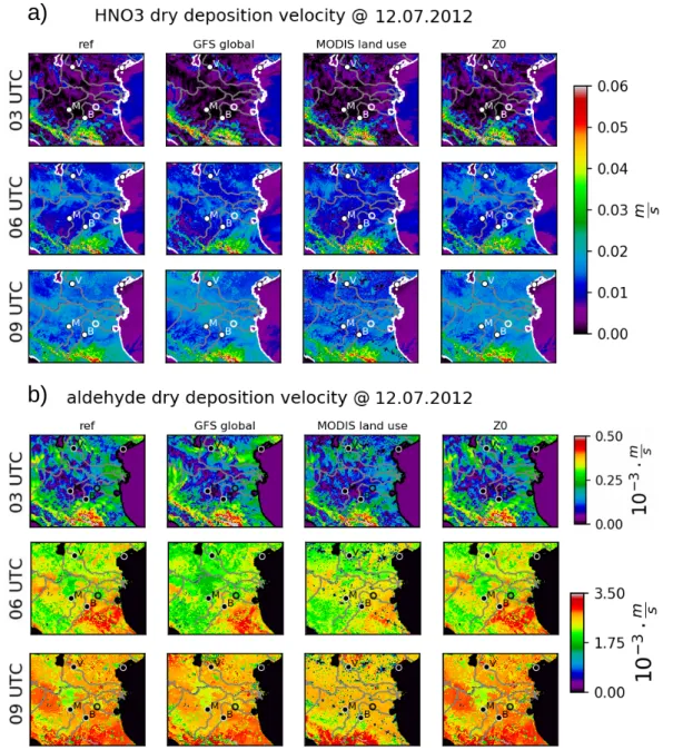
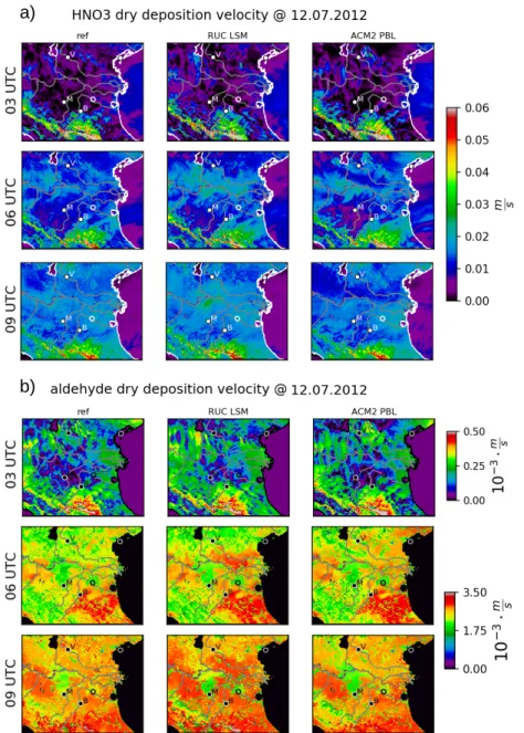
6.2 Dry Deposition Velocities . . . . 49

6.3 Dynamics . . . . 53

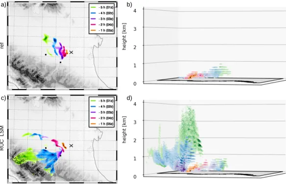
6.3.1 Source Regions . . . . 53

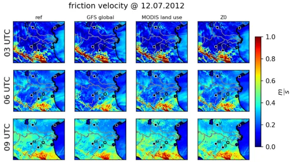
6.3.2 Friction Velocity . . . . 55

6.3.3 Surface Exchange Coefficients . . . . 57

6.4 Implications for KL Ensemble Perturbation . . . . 60

7 Ensemble Generation Results 61 7.1 Stochastic Biogenic Emissions . . . . 62

7.1.1 Full Input Sensitivities . . . . 62

7.1.2 Independent Input Sensitivities . . . . 67

7.1.3 Additional A-priori Uncertainties . . . . 69

7.2 Stochastic Dry Deposition Velocities . . . . 71

7.3 Stochastic Surface Exchange Coefficients . . . . 74

8 Ensemble Performance 79 8.1 Joint Perturbation . . . . 79

8.2 Ensemble Validation by Flight Observations . . . . 86

8.2.1 Vertical Flight on 12.07.2012 . . . . 86

8.2.2 Horizontal Flight on 01.07.2012 . . . . 88

8.2.3 Evening Flight on 07.07.2012 . . . . 92

8.3 Computational Scaling . . . . 96

9 Conclusion and Outlook 99 A Flowcharts WRF parameterization schemes 102 A.1 Flowchart Eta surface layer scheme in WRF . . . 102

A.2 Flowchart MYJ boundary layer scheme in WRF . . . 102

B Appendices Development KL Ensemble 104 B.1 Proof of Random Coefficients . . . 104

B.2 Discrete Eigenvalue Problem . . . 104

B.3 Random Number Generation . . . 105

C Implementation of KL Ensemble in EURAD-IM 106 C.1 Namelist Parameters . . . 106

C.2 Structure . . . 107

C.3 Initialization . . . 108

C.4 Generation of KL Perturbations . . . 109

C.5 Application of Perturbations . . . 110

D Derivation of Mean Values and Covariances for Independent Factors 112

D.1 Definition of the Problem . . . 112

D.2 Mean Values . . . 112

D.3 Covariances . . . 113

E Modified Roughness Lengths in WRF 115 F Appendix Sensitivity Analysis 116 G Appendices KL Ensemble Results 117 G.1 Appendix KL Ensemble Results for Biogenic Gases . . . 117

G.1.1 Setup of Full Sensitivities . . . 117

G.1.2 Additional Results for Independent Sensitivities . . . 118

G.1.3 Additional Results for Additional A-priori Uncertainties . . . 119

G.2 Additional Results for Dry Deposition Velocities . . . 121

G.3 Results for Friction Velocities . . . 124

G.4 Additional Results for Surface Exchange Coefficients . . . 126

Bibliography 129

Index 141

Numerical atmospheric models rely on assumptions about the atmospheric system, which lead to errors in model forecasts. Nevertheless, these models are widely used to provide weather forecasts on an operational basis. Additionally, atmospheric models play an im- portant role in various research fields, such as meteorological hazards, air quality and climate change. Much effort has been made to improve atmospheric forecast models in order to increase the reliability of their forecasts. However, these improvements result in a continuously increasing number of variables and considered processes. Although increas- ing the models complexity improves forecasts, atmospheric models remain approximations of the high-dimensional dynamical system.

The use of data assimilation techniques aims to reduce some of these uncertainties by pushing relevant quantities towards their observed equivalent. These optimization quantities are assumed to be highly uncertain and have significant impact on the forecast, but can be constrained by available observations. Although the benefit of advanced data assimilation for atmospheric forecasts has been demonstrated for various applications (e.g.

Daley [1993]; Kalnay [2003]; Sandu and Chai [2011]; Lahoz and Schneider [2014]), the use of observations and assumptions in the assimilation procedure induce additional sources of uncertainties to the system (e.g. Buizza [2019]).

Generally, every part of the modeling system introduces potential uncertainties to the forecasts. The question is how these uncertainties can be quantified realistically. The specific estimation of forecast uncertainties depends on the actual context. This study introduces an approach for uncertainty estimation of atmospheric forecasts considering three different aspects: Theoretical developments in the context of predictability, techni- cal implementation into chemistry transport models and specific application to biogenic gases. The objectives arising from each of these aspects are consecutively motivated in the following.

From a theoretical point of view, the question of predictability estimates forecast uncertainties. Due to the atmosphere’s highly nonlinear behavior, forecast uncertainties vary significantly in space and time and differ between variables. In general, atmospheric forecasts are sensitive to uncertainties originating from different types of sources. On the one hand, errors might be introduced by uncertainties in any kind of input – like initial fields and boundary conditions (e.g. Kalnay [2003]; Buizza et al. [2005]). On the other hand, inaccuracies in the formulation of the model itself contribute to forecast uncertainty. These model uncertainties may originate from predefined model parameters, simplified formulations of processes as well as the numerical implementation (e.g. Buizza et al. [1999]; Shutts [2005]).

Different approaches for an analytical formulation of model uncertainties are known

in mathematics (see Sec. 2.1). However, the high dimensionality of atmospheric models

makes an analytical formulation of probability densities computationally impracticable (e.g. Ehrendorfer [2006]; Kalnay [2019]). Instead, a set of deterministic forecasts is per- formed to approximate the probability distribution of the forecast state in numerical weather prediction (NWP). Each member of this ensemble of forecasts may be driven by slightly perturbed model inputs or model formulations which represent related uncertat- intes.

However, the generation of the ensemble is crucial as it determines the forecast prob- ability distribution. At the same time, the number of ensemble members for such high- dimensional systems is limited by computational resources. The major challenge is the generation of ensembles which sufficiently sample the forecast uncertainty with manage- able computational effort. Bauer et al. [2015] state that ensemble forecasting is still one of the most challenging research areas in numerical weather prediction. Additionally, a physically based uncertainty estimation may give also insight into model deficiencies (e.g.

Xian et al. [2019]). Thus, it can help to further improve the forecast model.

Regarding uncertainties in model parameters, perturbations are usually applied to the whole parameter field or to each location and time separately. However, constant perturbation of the whole parameter field does not allow for any spatial variation. In contrast, independent perturbation of each location and time becomes impractical for high-dimensional systems. Toth and Kalnay [1993] and Palmer [2019] state that sufficient uncertainties in initial conditions cannot be achieved by arbitrary, random perturbations of individual quantities.

Translating this to parameter uncertainties, this study introduces an approach to per- turb model parameters in an efficient way. Focusing on leading coupled uncertainty modes of multiple parameters, the developed ensemble algorithm aims to cover the dominating uncertainties even with a small ensemble size.

Regarding atmospheric modeling systems, chemistry transport models (CTMs) provide forecasts of atmospheric composition including a large set of trace gases and aerosol compounds. This large number of prognostic variables leads to high dimension- ality of the system even compared to NWP (e.g. Zhang et al. [2012a]). Among other implications, this high dimensionality amplifies uncertainties which differ significantly be- tween individual chemical compounds (Emili et al. [2016]). At the same time, multiple interactions by chemical reactions also induce multi-variational correlations of model state and errors.

CTMs are typically driven by NWP forecasts and thus inherit their errors. Besides that, prominent uncertainties of chemical forecasts arise from errors in estimations of emissions, chemical mechanisms and reactions as well as deposition and sedimentation processes. In most cases, the atmospheric composition is mainly determined by balances between emission and deposition processes. Thus, CTMs can be more sensitive to uncer- tainties in model parameters than initial- and boundary conditions (Elbern et al. [2007];

Bocquet et al. [2015]). However, there are only few attempts for estimating parameter uncertainties within CTMs (see Sec. 2.3). Low level chemical composition is especially sensitive to local transport and mixing within the atmospheric boundary layer. This en- hances a general dependency of air quality forecasts on the accuracy of NWP. Zhang et al.

[2012b] argue that a (from a meteorological point of view) optimal NWP forecast may

cover the whole lifecycle of multiple chemical compounds. This is achieved by accounting for chemical parameters – in form of emissions and deposition velocities – on the one hand, and meteorological parameters – determining local transport – on the other hand.

From an atmospheric chemical point of view, biogenic gases like biogenic volatile organic compounds (BVOCs) are subject to highly complex formulations and chemical transformations. On the one hand, there is a huge number of volatile organic compounds (VOCs) with fairly low concentrations in the atmosphere (e.g. Goldstein and Galbally [2007]). Being highly reactive, VOCs affect air quality and climate change via formation of aerosols and ozone (see Sec. 2.4). On the other hand, estimations of biogenic emissions rely on rough assumptions about the terrestrial ecosystem. The emitted amount of single BVOC is highly sensitive to local vegetation and surface properties. In CTMs, these properties are usually subject to high uncertainties in terms of their spatial distribution and temporal evolution.

The complexity and variability of biogenic gases motivates the investigation and mod- eling of related uncertainties. Uncertainties due to multiple dependencies of biogenic emissions and deposition velocities are considered. Based on this, a quantitative and state-dependent uncertainty estimation is achieved for biogenic gases.

The overall purpose of this study arises from the individual objectives described above and can be summarized as follows: (1) Development of an ensemble algorithm for efficient parameter perturbation in atmospheric models focusing on leading coupled uncertainties.

(2) Implementation for uncertainties in emissions, transport and deposition covering the whole lifecycle of chemical compounds. (3) Application to biogenic gases with highly state-dependent uncertainties.

Ch. 2 gives a short literature overview including existing approaches in uncertainty

estimation and the mathematical basis for the developed algorithm. The model environ-

ment in which this work is embedded is described in Ch. 3. Based on this, Ch. 4 describes

the development of the ensemble algorithm. The case study to which the ensemble al-

gorithm is applied is introduced in Ch. 5. Results from a sensitivity analysis and the

ensemble generation are given in Ch. 6 and 7, respectively. Finally, Ch. 8 evaluates the

performance of ensemble forecasts and Ch. 9 concludes this study.

The predictability of numerical forecasts of dynamical systems is generally limited. This is caused by sources of uncertainties which may be related to both, imperfect input parameters and uncertainties in the numerical model.

This chapter presents a literature overview including established approaches to pre- dictability of numerical forecasts. Sec. 2.1 introduces basic ideas for probabilistic forecasts from a mathematical point of view. Specific approaches for uncertainty estimations for numerical weather prediction and chemistry transport modeling are shortly described in Sec. 2.2 and 2.3, respectively. Sec. 2.4 gives a short introduction to biogenic gases. A theoretical description of the Karhunen-Lo´ eve expansion – which serves as basis for the approach developed during this study – is given in Sec. 2.5.

2.1 Mathematical Basis

In the following, mathematical approaches for probabilistic forecasts in terms of prob- ability density functions (PDF) and covariances are shortly introduced. For a detailed overview see for example Xiu [2010].

Forecast of PDF in Phase Space

The Liouville equation known from Hamiltonian mechanics can be used to describe the temporal evolution of the models PDF in phase-space (compare e.g. Epstein [1969];

Ehrendorfer [2006]). It can be expressed by a continuity equation of the probability ρ(x, t) of the model state x at time t

∂ρ(x, t)

∂t + X

i

∂ [ρ(x, t) ˙ x

]

∂x

= 0 (2.1)

With this, the Liouville equation can be interpreted in the way that the probability ρ is constant along a model trajectory in phase-space.

The Fokker-Planck equation considers additive white noise to account for model un- certainties in the Liouville equation

∂ρ(x, t)

∂t + X

i

∂

∂x

[ρ(x, t) ˙ x

] + X

i

X

j

∂

∂x

τ

2

∂ρ(x, t)

∂x

= 0 , (2.2)

where τ

j is the variance of the white noise describing the stochastics. The Fokker-Planck

equation provides a theoretical formulation of the probabilistic evolution of uncertainties

in time. However, applying the approach to discrete systems becomes computationally

prohibitive even for dimensions far below the ones of atmospheric systems (e.g. Hunt et al. [2007]).

Linear Forecast of the Error Covariance Matrix

As numerical models are formulated in finite-dimensional phase states, a discrete approach to forecast model uncertainties via covariances is presented. For a non-linear model M, the related forecast x

starting from an initial state x

at time t < t

is given by

x

= M

(x

) + ε

, (2.3) where errors ε

in the forecasted state at time t

are induced by both, errors in the initial state x

and imperfect formulation of the numerical model M

.

Assuming the existence of a linear approximation of the model, the covariance matrix of the forecast C

can be calculated using the linearized model M

and its transposed M

(e.g. Daley [1993])

C

= M

C

M

. (2.4) This approach requires the knowledge of the covariance matrix C

at initial time t. It does only account for the development of initial uncertainties given by C

. In order to consider model uncertainties as well, a model error covariance matrix Q is included as additive term

C

= M

C

M

+ Q . (2.5) This propagation of error covariances is used in the theoretical formulation of the Kalman-filter algorithm for calculating the forecast covariances required for data assimi- lation. However, the matrix multiplication limits this approach to low-dimensional prob- lems where the size of the matrices is treatable.

2.2 Atmospheric Ensemble Approaches

Early attempts to uncertainty quantification for NWP systems were focusing on sensi- tivities to initial conditions (e.g. Thompson [1957]). Already in the beginning of the 20

century, Poincar´ e denoted the existence of deterministic chaos which describes the random evolution of uncertainties by imperfect initial conditions even for a perfect model (Poincar´ e [1914]). This behavior became popular as butterfly effect based on the studies of Lorenz [1963].

Leith [1974] introduced the idea of Monte-Carlo forecasts as an ensemble of randomly

perturbed atmospheric forecasts according to Gaussian PDFs. Following his idea, different

ensemble approaches are currently used on operational NWP systems. The most popular

ones dealing with uncertainties in initial conditions or the forecast model are shortly

described below.

Initial Value Uncertainties

For uncertainties in initial conditions, Bred vectors (Toth and Kalnay [1993]) or Singular vectors (Buizza et al. [1993]) are used to detect directions of the fastest growing initial uncertainties over a given time interval. Both approaches aim for generating an efficient ensemble covering the largest uncertainties caused by initial conditions. Another approach estimates uncertainties in initial values by applying random perturbations to observations (PO) which are assimilated into the model (e.g. Houtekamer et al. [1996]).

The singular vector (SV) approach developed by Buizza et al. [1993] provides linear estimates of the directions of fastest growing uncertainties. The idea is to detect sensitive system states with large potential for amplification in time. This is achieved by calculating the singular value decomposition of the linear model M

M = U · Σ · V

, (2.6)

with Σ the diagonal matrix of singular values and U , V being matrices containing the left and right singular vectors, respectively. The length of the time integration by M determines the timescale on which the perturbations are acting (e.g. Sandu et al. [2005]).

Here, the singular vectors related to the largest singular values provide the directions of fastest growing initial uncertainties. These directions are scaled by assumed sizes of uncertainties to generate a set of perturbed initial fields.

However, the singular value decomposition requires a local linearization of the often highly nonlinear model operator M around the most likely model state. This limits the SV approach to the linear regime around the model state (e.g. Hoffman and Kalnay [1983]) in terms of size of perturbations and forecast time. Additionally, the singular vectors – and therefore also the perturbations – appear to be sensitive to the considered time-interval.

To avoid the linearization of the model, the Breeding approach was introduced by Toth and Kalnay [1993]. The approach arises from the idea that the directions of fastest growing perturbations naturally develop in the data assimilation process (e.g. Buizza et al. [2005]). Therefore, Bred vectors (BVs) are determined from the differences between two forecast. For a repetitive integration of these differences in time, BVs tend to convert to low dimensional subspaces related to the most uncertain directions (e.g. Toth and Kalnay [1993]). At this time, the BVs become independent of the direction of the initial differences. Thus they can be seen as a nonlinear formulation of the leading Lyapunov vectors (e.g. Kalnay [2003]; Buizza et al. [2005]). Finally, stochastic initial fields are created by adding or subtracting perturbations according to the direction of the leading BVs.

Model Uncertainties

Studies have shown that errors in initial conditions are not able to explain forecast un-

certainties completely (e.g. Buizza et al. [2005]). The formulation of NWP models itself

appears to be another important source of uncertainties. Moreover, model uncertainties

trigger initial uncertainties of the ensuing forecast (e.g. Lock et al. [2019]). The two most

common types of approaches for model uncertainties are described below.

The first group of methods is related to uncertainties in model parameterizations.

These parameterizations rely on simplified assumptions about subgrid-scale processes, which have significant impact on resolved scales. Houtekamer et al. [1996] multiplied random numbers to parameters of parameterization schemes. In this stochastic parameter perturbation (SPP) approach, selected parameters in the single parameterization schemes are perturbed according to assumed uncertainties. Thus, uncertainties in the outcome of the parameterizations due to uncertain parameters are featured. Usually, these pertur- bations are applied to the whole parameter field or to each location and time separately.

On the one hand, perturbing the whole parameter field does not allow for any spatial variation and is therefore not able to represent local state-dependent uncertainties. On the other hand, applying perturbations to different locations and times separately suffers from the high dimensionality of the system. Even introducing predefined dependencies to neighboring locations requires a large ensemble size and may not produce reasonable perturbations (e.g. Toth and Kalnay [1993]).

In contrast, Buizza et al. [1999] introduced the stochastically perturbed parameteriza- tion tendencies (SPPT) scheme. This approach considers uncertainties in the formulation of the parameterization schemes itself. Instead of perturbing parameters, the total tenden- cies p

of state variables from all parameterizations are perturbed. These total tendencies are multiplied with random numbers r sampled from an arbitrary PDF by

p = (1 + r) p

, (2.7)

thus the underlying uncertainties are assumed to be proportional to the total tendency.

By perturbing total tendencies resulting form all parameterizations, the balance between different processes is not affected (e.g. Palmer [2019]). Although perturbations are gen- erated in a spatially and temporally correlated way, both correlation scales and standard deviations of the random numbers are predefined as a fixed value (e.g. Leutbecher et al.

[2017]; Lock et al. [2019]).

The stochastic kinetic energy backscatter scheme (SKEBS, Shutts [2005]) represents a different group of methods focusing on another source of model uncertainty. It is based on the need to account for energy backscattering from subgrid-scales to resolved scales in order to balance energy dissipation (e.g. MacVean [1983]). This two-way exchange of kinetic energy considering subgrid-scale energy sources is assumed to be of stochastic nature (e.g. Shutts [2005]). In SKEBS, stochasticity is realized by adding random noise to the prognostic equation of the stream-function. Where the random noise is proportional to the total energy dissipation rate, multiplied by random numbers. In Shutts [2005], a cellular automaton ensures predefined temporal and spatial correlations of the random numbers within a fixed range.

2.3 Uncertainties in Chemistry Transport Model- ing

In chemistry transport modeling, the sensitivity to uncertain model parameters is much

more dominant compared to NWPs. Generally, potential sources of uncertainties in CTMs

may be introduced through the whole lifecycle of each compound (for an detailed overview see e.g. Zhang et al. [2012b]). Specifically, chemical sources to the atmosphere in the form of emissions are subject to large errors concerning the spatial and temporal distribution (e.g. Elbern et al. [2007]). Within the atmosphere, chemical compounds are influenced by the atmospheric environment depending on meteorological conditions and reactive chemistry with other compounds including gas-phase chemistry, photolysis and aerosol chemistry (e.g. Bocquet et al. [2015]; Emili et al. [2016]). Finally, different kinds of de- position and sedimentation processes acting as chemical sink also contribute to forecast uncertainties (e.g. McKeen et al. [2007]; Wu et al. [2015]). The longer the forecast hori- zon, the more are chemical forecasts determined by emission and deposition processes compared to initial conditions (e.g. Elbern et al. [2007]; Bocquet et al. [2015]). Addition- ally, the general sources of uncertainties in atmospheric models like initial- and boundary conditions as well as the numerical implementation do also apply to CTMs. Besides an uncertainty estimation by multi-model ensembles (e.g. McKeen et al. [2007]; Xian et al.

[2019]), there are only few attempts for ensemble generation within a single CTM.

Recent attempts follow two different strategies to account for uncertainties in CTMs.

Firstly, former studies aim to account for uncertainties in model parameters or other chemical input fields (compare e.g. Zhang et al. [2012b]). Again, perturbing parameter fields appears to suffer from the high dimensionality of the system. Early studies like the one performed by Hanna et al. [1998] assume predefined uncertainties where per- turbations are applied uniformly in space and time, and ignoring any cross-correlation between parameters. This uniform perturbation of model parameters with a fixed stan- dard deviation is still applied to emissions in the context of ensemble data assimilation (e.g. Schutgens et al. [2010]; Candiani et al. [2013]). However, already Hanna et al. [1998]

state that introducing state-dependency of uncertainties and cross-correlations between parameters would provide a more realistic representation. More recently, limited spatial correlations are considered in uncertainty estimation by uniform perturbations within arbitrary subregions (Boynard et al. [2011]; Emili et al. [2016]) or isotropic decrease with fixed correlation length scales (e.g. Gaubert et al. [2014]).

Secondly, Vautard et al. [2001] were the first creating an ensemble of ozone forecasts by driving the CTM with an existing meteorological ensemble. This comparably simple approach is based on the assumption that chemical forecasts are more sensitive to meteo- rology than to chemical uncertainties due to emissions or reactive chemistry (e.g. Zhang et al. [2012b]). In general, uncertainties in NWP may induce uncertainties in CTMs by multiple dependencies. For example, chemical compounds are found to be sensitive to wind fields, temperature, clouds, water vapor and precipitation (e.g. Hess et al. [2004];

McKeen et al. [2007]). Near-surface chemical composition is additionally sensitive to the structure of the boundary layer, for example controlling the boundary layer height, sta- bility, turbulence and surface fluxes (e.g. Hess et al. [2004]; Eder et al. [2006]; Banks et al.

[2016]).

2.4 Biogenic Volatile Organic Compounds

Although occurring in small concentrations, there is a huge number of non-methane volatile organic compounds (VOCs) in the atmosphere – and even more compounds are still expected to be found (e.g. Goldstein and Galbally [2007]). VOCs play an active role in tropospheric chemistry, with essential implications for air quality and climate change.

On the one hand, VOCs contribute significantly to formation of secondary organic aerosols (SOA, e.g. Geng et al. [2011]; Shrivastava et al. [2017]). SOA act as cloud condensation nuclei and therefore affect aerosol-cloud interaction (e.g. Shrivastava et al. [2017]). On the other hand, VOCs are an important component in the photochemical production of tropospheric ozone (e.g. Geng et al. [2011]; Wu et al. [2015]).

A large fraction of VOCs in the atmosphere is emitted by the terrestrial ecosystem (e.g. Lamarque et al. [2010]). Compared to anthropologically emitted compounds, these biogenic VOCs (BVOCs) are especially sensitive to meteorological conditions. Addition- ally to the interaction with the atmospheric environment, the emission process of BVOCs is highly dependent on various atmospheric, vegetation- and soil-related properties. Ex- amples for these dependencies are solar radiation, air temperature, soil moisture and biomass density (e.g. Lavoir et al. [2009]; Wu et al. [2015]). Moreover, biogenic emissions as well as dry deposition velocities vary significantly between different vegetation types (e.g. Wesely and Hicks [2000]; Wu et al. [2015]).

With an approximated contribution of about 50%, isoprene is the most dominant BVOC in terms of global annual emissions (Guenther et al. [2012]). In contrast to other BVOCs, isoprene is a direct product of the plants biosynthesis (e.g. Wu et al. [2015]).

It has comparably high OH-reactivity (e.g. Fuentes et al. [2000]; Wang et al. [2017]) resulting in a lifetime of about 30 minutes, which is shorter than for other BVOCs (see e.g. Carslaw et al. [2000]; Geng et al. [2011]). The short lifetime of isoprene limits the gas to the local surrounding of the emission location. Therefore, its spatial and temporal distribution may be highly variable with considerable horizontal variations on the order of kilometers (e.g. Guenther et al. [2006]; Wang et al. [2017]).

The huge variability and highly complex dependencies render the modeling of bio-

genic gases nontrivial. This results in large differences in modeled monoterpene emissions

reported for example by Arneth et al. [2008]. Estimates of global uncertainties in bio-

genic emissions range from a factor of two (Lamb et al. [1987]) to one order of magnitude

(Hanna et al. [2005]). Furthermore, uncertainties in biogenic gases induce uncertainties

in their chemical products like SOA and ozone formation (Shrivastava et al. [2017]). In

contrast, dry deposition velocities of all chemical compounds – including chemical prod-

ucts of BVOC like ozone – differ by about 30% between different models (Wesely and

Hicks [2000]).

2.5 Karhunen-Lo´ eve Expansion

The Karhunen-Lo´ eve (KL) expansion - named after Karhunen [1947] and Lo´ eve [1948] - decomposes a stochastic process into a linear combination of a set of random variables.

The KL approach is used in a various fields of applications (compare Wang [2008]). In the context of meteorological data analysis without the stochastic application, its discrete form is called empirical orthogonal functions (EOFs) and refers to a principal component analysis (PCA) of datasets (eg. Galin [2007]).

A more detailed description of the applied numerical methods can be found in Xiu [2010], the notation of which is adopted in this study.

Let x(ω, s) be a stochastic process with random dimension ω ∈ Ω and location s ∈ S with S the spatial dimension. The underlying idea is to describe the stochastic process as a linear combination of products of deterministic and stochastic elements

x(ω, s) =

∞

X

d=1

f

(s) y

(ω) , (2.8)

with pairwise-uncorrelated deterministic functions f

(s) and pairwise-uncorrelated stochas- tic coefficients y

(ω).

Eq. (2.8) holds for stochastic processes which are centered around zero. If the original distribution does not fulfill this criterion, the stochastic process is shifted by its mean value x(s) = e x(ω, s) − µ(s).

The vectors of stochastic coefficients y

(ω) are defined to be orthogonal to each other.

They need to be sampled from a PDF fulfilling the following properties (compare Ap- pendix B.1):

• The expectation value is zero.

• The standard deviation is given by square root of eigenvalues λ

. Thus, y

(ω) can be written as

y

(ω) := p

λ

Y

(ω) , (2.9)

which gives the following conditions for the normalized stochastic coefficients Y

(ω) E [Y

(ω)] = 0 ∀ d , E [Y

(ω) Y

(ω)] = δ

∀ d, d

, (2.10) where δ

is the Kronecker delta.

The selected distribution of the stochastic coefficients takes a similar form as the

desired distribution of the stochastic process. In case of a Gaussian stochastic process,

the stochastic coefficients are also Gaussian distributed. For other distributions, the

definition of the stochastic coefficients becomes much more complicated. Schwab and

Todor [2006] mentioned that the assumption of independent stochastic coefficients Y

(s)

might not always be justified which induces an additional error.

The KL approach offers the possibility to use spatial correlations of the stochastic process x(ω, s) given by their covariance. By interpreting the deterministic functions as eigenfunctions of the covariances ϕ

(s) and using Eq. (2.9), the KL expansion reads:

x(ω, s) =

∞

X

d=1

p λ

ϕ

(s) Y

(ω) , (2.11)

where Y

(ω) are normalized stochastic coefficients.

The eigenvalues λ

and eigenfunctions ϕ

(s) are determined by the integrative covari- ance matrix C(s, s

) := E [x(ω, s) x(ω, s

)] of the stochastic process, with s, s

∈ S

Z

S

C(s, s

) ϕ

(s

) ds

= λ

ϕ

(s) . (2.12) This eigenvalue problem is usually replaced by an eigenvalue problem of a linear operator defined as

T

(s) : f → T

(s) · f = Z

S

C(s, s

) f (s

) ds

. (2.13) As correlations in C(s, s

) are generally symmetric and positive definite, the linear operator is compact and self-adjoint (Schwab and Todor [2006]).

The practical computation of Eq. (2.11) requires a finite approximation of the KL expansion. By defining a finite truncation D < ∞, the KL approximation becomes

x(ω, s) ≈

D

X

d=1

p λ

ϕ

(s) Y

(ω) . (2.14) In order to archive an minimal error induced by the truncation, the eigenvalues and related eigenfunctions are sorted by their values: λ

≥ λ

≥ · · · ≥ λ

. Thus, the first terms contribute most to the stochastic process. The determination of the truncation limit depends on the decay of the eigenvalues and the acceptable error induced by the algorithm.

The main feature of the KL expansion is that a stochastic process is decomposed into orthogonal functions with stochastic coefficients. Thus, KL can be seen as a stochastic extension to Fourier series (eg. Wang [2008]). The determination of the coefficients is optimal in a mean square sense by minimizing the mean square error of the finite representation (eg. Schwab and Todor [2006]). The only required information on the stochastic process are its stochastic mean µ(s) = x(s) and covariances C(s, s

). Given this, the KL approximation samples from a subspace of the stochastic space which is given by the covariances. In this context, the leading eigenvalues and corresponding eigenfunctions provide the size and direction of the major uncertainties of the stochastic process, respectively.

The main advantage of the KL algorithm is the consideration of correlations of the

stochastic process. First of all, the correlation of the process limits the error of the finite

approximation (eg. Xiu [2010]). As it can be seen in Fig. 2.1, the higher the correlation the faster is the decay of its eigenvalues. This leads to a lower error for a fixed truncation limit or to a lower truncation limit for a fixed error. Thus, the correlated field of stochastic processes can be decomposed into a small number of uncorrelated elements (principal components, Hotelling [1933]). Moreover, the low number of principal components only requires a reduced number of stochastic coefficients as they are used globally for all s ∈ S.

The reduced dimension of the problem becomes especially important for high dimensional systems being generally limited by computational resources.

Figure 2.1: Decreasing behavior of leading eigenvalues for exponential covariances with different

correlation length

taken from Fig. 4.2 in Xiu [2010].

This chapter presents an overview of the pre-existing modeling framework on which the developments for this study are based. Three linked modeling systems are used or further developed. On the one hand, the ensemble generation algorithm was applied to two limited-area atmospheric models. While perturbations of meteorological model parame- ters are considered in WRF (Sec. 3.1), atmospheric chemical parameters are handled in EURAD-IM (Sec. 3.2). The description of both modeling systems focuses on those mod- ules, which are important for the developments performed during this study. On the other hand, an existing ensemble environment for WRF and EURAD-IM is shortly described in Sec. 3.3. Although this ensemble environment was not completely adopted, some parts are used in this study.

3.1 WRF Numerical Weather Prediction System

The WRF (Weather Research and Forecasting ) model is a mesoscale numerical weather prediction model, which originates from a joint coordination effort of NCAR (National Center for Atmospheric Research), NOAA (National Oceanic and Atmospheric Adminis- tration), the U.S. Air Force, the Naval Research Laboratory, the University of Oklahoma and the Federal Aviation Administration. Its code is freely accessible and widely used for various applications. WRF offers two dynamical cores NMM (Nonhydrostatic Mesoscale Model ) and ARW (Advanced Research WRF ) as well as additional packages including data assimilation (WRFDA) and atmospheric chemistry (WRF-Chem). A detailed description can be found in Skamarock et al. [2008].

In this study, the WRF-ARW version 3.8.1 is used. The WRF framework consists of a sequence of components allowing for a flexible and comfortable preparation of intended simulations. On a first level, the system can be divided into the WRF Preprocessor System WPS and the WRF system. On a second level, WPS consists of three individual compo- nents. Firstly, GEOGRID defines the grids and interpolates terrestrial information for all required domains. Secondly, UNGRIB prepares the meteorological input files for the sim- ulation time. Thirdly, METGRID interpolates the prepared meteorological information for the current domain.

The WRF system is fully parallelized and includes the final preparation of initial-

and boundary conditions in REAL as well as their interpolation to nested domains in

NDOWN. Finally, the forecast of WRF-ARW is performed by solving fully compressible

non-hydrostatic prognostic equations. The vertical grid is defined by terrain-following

hydrostatic-pressure coordinates and the prognostic variables are horizontally staggered

in an Arakawa-C-grid (Arakawa and Lamb [1977]) stencil. Time integration is performed

by the 2

or 3

order Runge-Kutta scheme.

Multiple schemes for various kinds of parameterizations are available in the WRF model. Available parameterizations account for subgrid-scale processes related to the boundary- and surface layer, land- and urban surface, lake physics, short- and longwave radiation, cloud microphysics and cumulus parameterizations. This study focuses on parameters handled by the boundary- and surface layer schemes as well as the land surface model. Reference options of the parameterization schemes – in which the perturbation of model parameters are implemented during this study – are described in more detail below.

3.1.1 Boundary Layer Parameterization

In numerical weather prediction models, boundary layer parameterizations approximate subgrid scale processes in the planetary boundary layer (PBL). As these processes often have a high spatial and temporal variability, boundary layer parameterizations have to provide reasonable averages over a potentially large scale. Different parameterization schemes are based on different assumptions about the treatment of transport, moisture and energy in the PBL (e.g. Hu et al. [2010]). Additionally, these schemes include numer- ous tuneable parameters, which may be calibrated with a limited number of observations restricted to one specific region (Yang et al. [2016]). Therefore, one primary source of uncertainties in mesoscale atmospheric models is related to boundary layer parameteriza- tions. For example, Pleim [2007] reports significant errors in wind speeds for all considered parameterization schemes. Moreover, parameters describing the PBL structure like the boundary layer height (BLH) may also be defined in different ways. These parameters may have especially significant influence for the dispersion of pollutants in atmospheric chemical simulations.

Technically, boundary layer parameterizations approximate mean profiles of atmo- spheric state variables or their tendencies in the PBL. In general, currently used param- eterization schemes can be classified into two approaches. On the one hand, local closure schemes are based on K-theory, where the subgrid scale turbulent flux is assumed to be proportional to the local gradient (Stull [1988]). Current local schemes are usually of 1.5

or 2

order including more detailed formulations than the 1

order K-theory. 1.5

order schemes like MYJ (Mellor-Yamada-Janjic, Janjic [1994]), BouLac (Bougeault-Lacarrere, Bougeault and Lacarrere [1989]) or MYNN (Mellor-Yamada-Nakanishi-Niino, Nakanishi and Niino [2006]) use an additional prognostic equation for the mean turbulent kinetic energy (TKE). 2

order schemes include prognostic equations for flux terms, which re- quire the parameterization of 3

order terms.

On the other hand, non-local closure schemes consider information from surrounding

locations or the whole vertical profile to approximate fluxes. Ideally, this approach is more

suitable in convective conditions, where the turbulence is buoyancy-driven and vertical

gradients become neglectable (e.g Garratt [1994]). Due to the complexity introduced

by non-local effects, non-local schemes like YSU (Yonsei University, Hong et al. [2006])

or ACM2 (Asymmetric Convection Model version 2, Pleim [2007]) are often of 1

order

closure. Studies investigating the performance of local and non-local approaches do not

show a clear ranking for those. It appears that the performance of each scheme highly

depends on atmospheric conditions (e.g. Yang et al. [2016]).

The Mellor-Yamada-Janjic (MYJ, e.g. Janjic [1994]) scheme is a local 1.5

order boundary layer parameterization scheme based on Mellor and Yamada [1982]. As a TKE closure scheme, TKE is treated as additional prognostic state variable determining the eddy diffusion coefficients. In this approach, the diffusivity in the closure of the prognostic TKE equation depends on a master length scale. Being based on the local K-approach, vertical turbulent mixing is defined to be proportional to the eddy diffusion coefficient K

for ξ ∈ {momentum,heat,TKE} (Janjic [2001])

w

ξ

:= −K

∂ξ

∂z . (3.1)

Here, different formulations of the coefficients K

are used for momentum (K

), heat (K

) and TKE (K

). The boundary layer height is defined as the height where TKE reaches a threshold of 0.2

. A flowchart of the most important variables of the MYJ PBL scheme as implemented in WRF is given in Appendix A.2.

3.1.2 Surface Layer Parameterization

The surface layer is the lowest part of the PBL and represents the connection between the earth’s surface and the atmosphere. According to Stull [1988], the surface layer is defined as the region, where the variation of turbulent fluxes drops below 10% of their magnitude. Due to its direct interaction with the earth’s surface, vertical profiles of atmospheric state variables are dominated by large gradients. These gradients induce large fluxes of atmospheric parameters like momentum, heat and moisture between surface and atmosphere (e.g. Arya and Holton [2001]).

In WRF, the surface layer is assumed to be represented by the lowest model layer.

Surface layer schemes provide exchange coefficients and surface fluxes of heat and mois- ture, which are required by the boundary layer parameterizations and the land surface model. Due to close interactions with the boundary layer scheme, surface- and boundary layer schemes should be selected accordingly. Parameterizations of the surface layer are based on the Monin-Obukhov Similarity Theory (MOST) derived by Monin and Obukhov [1954]. By applying similarity theory, the approach defines scaling parameters to gain universal relations between dimensionless variables. In the surface layer, scaling param- eters for momentum, temperature and humidity are u

– defined as friction velocity –, Θ

and q

, respectively. Given these scaling parameters, the Obukhov length L can be calculated and is a measure of stability. It is defined as the height where shear production equals buoyancy destruction leading to zero net production of turbulent kinetic energy.

The Eta-similarity surface layer scheme (e.g. Janjic [1996]) has been developed to act as lower boundary for the MYJ boundary layer scheme. Over land, the roughness length is defined in a variable way, considering differences when applying to temperature and humidity (Zilitinkevich [1995]). Over water, a viscous sublayer is explicitly defined as the layer in which transport is only determined by molecular diffusion (Janjic [1994]).

Additionally, the Beljaars correction (Beljaars [1995]) has been applied, which introduces

a velocity scale for free convection w

. Thus, the adopted friction velocity is formulated as follows:

u

:= C

·

u

+ v

+ (β · w

)

, (3.2)

where C

is the momentum transfer coefficient, β a constant scalar and u and v the wind components in zonal- and meredional direction, respectively. The final calculation of surface fluxes, which are provided to the land surface model, is performed iteratively.

A flowchart of the most important variables of the Eta-similarity surface layer scheme as implemented in WRF is given in Appendix A.1.

3.1.3 Land Surface Model

The earth’s surface represents the lower boundary in atmospheric models. Xiu and Pleim [2001] state that the most important task of a land surface model (LSM) is the estimation of evaporation, which determines the partitioning between sensible and latent heat flux.

As the estimated evaporation is determined by local soil and vegetation properties, these parameters have significant effect on the development of the PBL (e.g. Garratt [1994]).

Therefore, LSMs are assumed to be especially important when mesoscale meteorological forecasts are applied to CTMs (e.g. Xiu and Pleim [2001]; Gilliam and Pleim [2010]).

In WRF, the earth’s surface is divided into water and land surfaces, which are treated separately. Land surface models provide parameterizations of land surface processes and their interaction with the atmosphere. Representing an important component in the earth system, LSMs interact with all other parameterizations. However, their implementation in WRF is one-dimensional and does not include horizontal exchange. Their major out- puts are surface fluxes of heat, moisture and momentum as well as upwelling short- and longwave fluxes, which are feed into boundary layer and radiation schemes, respectively.

Except for the thermal diffusion scheme, soil temperature and moisture are treated as prognostic variables in LSMs. In the thermal diffusion scheme, soil moisture is set to a fixed value that varies between land use types and seasons. This simplification makes the scheme unpractical for application to forecasts of biogenic gases, where emissions soil moisture-dependent. The number of soil layers ranges from two (Pleim-Xiu) to ten (CLM4 ). Examples for featured processes are multi layer snow (RUC, CLM4 ), frac- tional snow cover (Noah), frozen soil physics (Noah, RUC ) or an explicit consideration of vegetation (Pleim-Xiu, CLM4 ).

The Pleim-Xiu LSM (PX LSM, Pleim and Xiu [1995]; Xiu and Pleim [2001]) is a two- layer soil temperature and -moisture model. The surface layer is defined by a depth of 1 cm and the root zone layer in 1 m depth acting a slowly varying reservoir. The scheme consists of five prognostic equations with corresponding prognostic variables: soil surface temperature T

:= T

, lower layer temperature T

:= T

, volumetric soil moisture at the surface w

:= w

, volumetric soil moisture in the lower layer w

:= w

,

and the amount of canopy water W

(see Pleim and Xiu [1995]). The formulation of

the prognostic equations is based on a force-restore approach (Deardorff [1978]), where

the driving forces for temperature and moisture are the surface budgets of energy and

moisture, respectively. Evaporation is computed by the sum of direct contributions from

the soil and wet canopies and vegetative evapotranspiration. For the numerical integration of the prognostic equations, the semi-implicit Crank-Nicolson technique is adopted.

3.2 EURAD-IM Chemical Data Assimilation Sys- tem

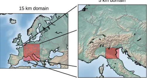
The atmospheric chemical data assimilation system EURAD-IM (EURopean Air pollution Dispersion - Inverse Model ) combines a state-of-the-art chemistry transport model with spatio-temporal data assimilation and inversion methods (Elbern et al. [2007]). The hor- izontal grid is created by a Lambert conformal projection where the prognostic variables are defined on a staggered Arakawa-C grid stencil (Arakawa and Lamb [1977]). In the vertical, model levels are given in terrain-following σ-coordinates. Additionally, sequen- tial one-way nesting may be applied to multiple nests, which enables the application of continental to local limited-area domains.

The chemistry transport model within EURAD-IM performs forecasts of a large set of gas phase and aerosol compounds up to lower stratospheric levels (e.g. Hass et al. [1995]).

The mass mixing ratio c

of any compound l is subject to different kinds of processes which are formulated as prognostic equation

∂c

∂t = −∇ (v c

) + ∇

ρ K e ∇ c

ρ

+ P

(c) + E

− D

(c

) , (3.3) with ρ the air density, v the 3-dimensional wind vector, K e the 3-dimensional eddy diffu- sivity tensor, P

(c) the net chemical production from all compounds c, E

the emission flux and D

(c

) the deposition flux of compound c

.

On the one hand, chemical compounds are influenced by dynamical transformations due to advective and diffusive processes. The advection schemes of Bott [1988] and Walcek [2000] are implemented in the model, of which the Bott scheme is used for this study. On the other hand, chemical production and destruction due to reactive chemistry with other compounds as well as photolysis are considered. Different options for gas- phase chemistry mechanism are implemented, which are all based on RACM (Regional Atmospheric Chemistry Mechanism, Stockwell et al. [1997]). For this study, the RACM- MIM (Geiger et al. [2003]) mechanism is selected which considers 221 chemical- and 23 photolysis reactions by 84 gases including condensed isoprene degradation (Mainz Isoprene Mechanism MIM, P¨ oschl et al. [2000]).

These processes build the core of the forecast model M. Due to the different time scales of the included processes, the model is implemented using symmetric operator splitting (Yanenko [1071])

M := D

1 2

h

T

1 2

h

T

1

v2

D

1

v2

C D

1

v2

T

1

v2

T

1 2

h

D

1 2

h

, (3.4)

with D

and T

the nonlinear horizontal/vertical operators for diffusion and advection,

respectively, and C the nonlinear chemistry module.

The dynamical processes related to diffusion and transport in horizontal and vertical direction are performed sequentially for half the model time step (denoted by the super- script

). The large range of time scales in the chemistry mechanism is handled by a sequence of small chemical time steps of variable length within C.

Additionally, emission and deposition fluxes represent the sources and sinks of chem- ical compounds, respectively. Emissions from anthropogenic- and biogenic sources are treated separately, where anthropogenic emissions provided by the TNO-MACC-II inven- tory (Kuenen et al. [2014]) are processed by the EURAD Emission module EEM (e.g.

Memmesheimer et al. [1991]). Dry and wet deposition is considered in the model, where wet deposition is included in the treatment of clouds. According to the focus of this study, the approximation of biogenic emissions and dry deposition are described in more detail in Sec. 3.2.1 and Sec. 3.2.2, respectively.

Besides gas phase chemistry, aerosols and pollen are also part of the model. Aerosol dynamics are realized by the MADE (Modal Aerosol Dynamics for Europe ), Ackermann et al. [1998] module where aerosols are separated by size into three modes. MADE includes multiple aerosol processes like nucleation, coagulation, particle growth and sedimentation.

Due to the coexistence of gases and aerosols, mixed-phase chemistry is also included.

In the EURAD-IM system, four-dimensional variational data assimilation (4Dvar) is implemented to identify initial fields x

and emission strengths of chemical compounds (Elbern et al. [2007]). The optimization of the emission strength is achieved via the definition of a field of emission factors e. It is assumed that the total amount, which is emitted at each location, is more uncertain than the quantitative diurnal cycle. Therefore, the emissions within the assimilation window [t

,t

] are multiplied by a constant factor, which can be optimized by data assimilation.

4Dvar is a spatio-temporal technique that estimates the best linear unbiased esti- mate (BLUE ). Model variables are optimized by minimizing a cost function J under the assumption of Gaussian error characteristics of the background model state (x

, e

) and observations (y

)

J (x

, e) = 1

2 x

− x

B

x

− x

+ 1

2 e − e

K

e − e

+ 1

2

tn

X

t=t0

h

H M

(x

)

− y

R

H M

(x

)

− y

i ,

(3.5)

with n

the number of model time steps in assimilation window, x

and x

the initial forecast and background state at initial time step t

, e and e

the forecast and background emission factors, y

the observations at time step t, M

the nonlinear forecast model operator (nonlinear), H the nonlinear observation operator, B and K background error covariance matrix for initial values and emission factors and R the observation error covariance matrix.

In the framework of data assimilation, the chemistry transport model M

acts as an operator transferring the model state at time t

to time t

x

= M

(x

) = M

◦ · · · ◦ M

x

. (3.6)