2 )inthePeruvianupwelling Theinfluenceofdissolvedorganicmatteronthemarineproductionofcarbonylsulfide(OCS)andcarbondisulfide(CS

https://doi.org/10.5194/os-15-1071-2019

© Author(s) 2019. This work is distributed under the Creative Commons Attribution 4.0 License.

The influence of dissolved organic matter on the marine production of carbonyl sulfide (OCS) and carbon disulfide (CS ₂ )

in the Peruvian upwelling

Sinikka T. Lennartz^1,a, Marc von Hobe², Dennis Booge¹, Henry C. Bittig³, Tim Fischer¹, Rafael Gonçalves-Araujo^5,10, Kerstin B. Ksionzek^4,6, Boris P. Koch^4,6,7, Astrid Bracher^8,10, Rüdiger Röttgers⁹, Birgit Quack¹, and Christa

A. Marandino¹

1GEOMAR Helmholtz Centre for Ocean Research Kiel, Marine Biogeochemistry, Düsternbrooker Weg 20, 24105 Kiel, Germany

2Forschungszentrum Jülich GmbH, Institute of Energy and Climate Research (IEK-7), Wilhelm-Johnen-Strasse, 52425 Jülich, Germany

3Leibniz Institute for Baltic Sea Research Warnemünde, Department of Physical Oceanography and Instrumentation, Seestraße 15, 18119 Rostock, Germany

4Alfred Wegener Institute Helmholtz Centre for Polar and Marine Research, Department of Biosciences, Ecological Chemistry, Am Handelshafen 12, 27570 Bremerhaven, Germany

5Aarhus University, Department of Bioscience, Frederiksborgvej 399, 4000 Roskilde, Denmark

6MARUM Center for Marine Environmental Sciences, Biogeochemistry, Leobener Straße, 28359 Bremen, Germany

7University of Applied Sciences, An der Karlstadt, 27568 Bremerhaven, Germany

8Institute of Environmental Physics, University of Bremen, 28334 Bremen, Germany

9Helmholtz-Zentrum Geesthacht, 21502 Geesthacht, Germany

10Alfred Wegener Institute Helmholtz Centre for Polar and Marine Research, Department of Climate Sciences, Physical Oceanography of the Polar Seas, Klußmannstr. 3d, 27570 Bremerhaven, Germany

anow at: Institute for Chemistry and Biology of the Marine Environment, University of Oldenburg, Oldenburg, Germany

Correspondence:Sinikka T. Lennartz (sinikka.lennartz@uni-oldenburg.de) Received: 17 January 2019 – Discussion started: 1 March 2019

Revised: 2 July 2019 – Accepted: 2 July 2019 – Published: 14 August 2019

Abstract. Oceanic emissions of the climate-relevant trace gases carbonyl sulfide (OCS) and carbon disulfide (CS₂) are a major source to their atmospheric budget. Their current and future emission estimates are still uncertain due to in- complete process understanding and therefore inexact quan- tification across different biogeochemical regimes. Here we present the first concurrent measurements of both gases to- gether with related fractions of the dissolved organic mat- ter (DOM) pool, i.e., solid-phase extractable dissolved or- ganic sulfur (DOS_SPE,n=24, 0.16±0.04 µmol L⁻¹), chro- mophoric (CDOM, n=76, 0.152±0.03), and fluorescent dissolved organic matter (FDOM, n=35), from the Peru- vian upwelling region (Guayaquil, Ecuador to Antofagasta, Chile, October 2015). OCS was measured continuously with

an equilibrator connected to an off-axis integrated cavity out- put spectrometer at the surface (29.8±19.8 pmol L⁻¹) and at four profiles ranging down to 136 m. CS₂ was measured at the surface (n=143, 17.8±9.0 pmol L⁻¹) and below, rang- ing down to 1000 m (24 profiles). These observations were used to estimate in situ production rates and identify their drivers. We find different limiting factors of marine photo- production: while OCS production is limited by the humic- like DOM fraction that can act as a photosensitizer, high CS₂production coincides with high DOS_SPEconcentration.

Quantifying OCS photoproduction using a specific humic- like FDOM component as proxy, together with an updated parameterization for dark production, improves agreement with observations in a 1-D biogeochemical model. Our re-

sults will help to better predict oceanic concentrations and emissions of both gases on regional and, potentially, global scales.

1 Introduction

Oceanic emissions play a dominant role in the atmospheric budget of the climate-relevant trace gases carbonyl sulfide (OCS) and carbon disulfide (CS₂) (Chin and Davis, 1993;

Kremser et al., 2016). OCS is the most abundant sulfur gas in the atmosphere, and CS2is its most important precursor.

Both gases influence the climate directly (OCS) or indirectly (CS2by oxidation to OCS in the atmosphere), as OCS is a major supplier of stratospheric aerosols (Brühl et al., 2012;

Crutzen, 1976), which exert a cooling effect on the atmo- sphere and can foster ozone depletion (Junge et al., 1961;

Kremser et al., 2016). Furthermore, OCS has been suggested as a proxy to constrain global terrestrial gross primary pro- duction (Campbell et al., 2008; Montzka et al., 2007; Berry et al., 2013). The oceanic emissions of both gases have recently attracted interest because they are suggested to account for a missing source of atmospheric OCS (Berry et al., 2013;

Kuai et al., 2015; Glatthor et al., 2015; Launois et al., 2015).

In situ measurements of OCS in surface seawater are still limited, but those available suggest that oceanic emissions are too low to fill the proposed gap of 400–600 Gg S yr⁻¹in the atmospheric budget (Lennartz et al., 2017). Still, oceanic emission estimates are associated with high uncertainties (ca.

50 %) (Kremser et al., 2016; Whelan et al., 2018). Reducing these uncertainties for present and future emission estimates requires (i) increasing the existing field data across various biogeochemical regimes and (ii) increasing process under- standing and quantification in the whole water column to fa- cilitate model approaches.

Most of the in situ observations of OCS and CS₂in sea- water were reported from the Atlantic Ocean and adjacent seas and mainly represent surface ocean measurements (see Whelan et al., 2018, for an overview). Here we report the first concurrent measurements in the surface ocean and the water column for both gases from the Peruvian upwelling. This re- gion is one of the most biologically productive regions in the global ocean due to the upwelling of nutrient-rich water.

The upwelling influences the pool of dissolved organic mat- ter (DOM) exposed to sunlight by transporting DOM from the deep ocean to the surface. The DOM pool is relevant in this context because it contains the precursors and pho- tosensitizers for the photochemical production of OCS and CS₂(Pos et al., 1998; Flöck et al., 1997; Uher and Andreae, 1997). Here we show measurements of chromophoric and fluorescent DOM as well as solid-phase extractable dissolved organic sulfur (DOS_SPE) in order to further specify drivers of production processes and improve parameterizations of pro- duction rates in biogeochemical models.

Chromophoric DOM (CDOM) is the fraction that absorbs light in the UV and visible range. CDOM contains photo- sensitizers that absorb light and facilitate photochemical re- actions, and it can undergo photodegradation itself (Coble, 2007). A part of the CDOM fraction fluoresces (FDOM), i.e., emits absorbed light at a shifted wavelength. Distinct groups of molecules have a specific fluorescence pattern, en- abling the molecule classes such as humic substances or pro- teins (FDOM components) to be differentiated (Coble, 2007;

Murphy et al., 2013). DOS_SPE is operationally defined as the dissolved organic sulfur retained by solid-phase extrac- tion (Dittmar et al., 2008). The method favors the retention of polar molecules, which comprise approximately 40 % of the total dissolved organic carbon (DOC) in marine waters (Dittmar et al., 2008). Due to the operational definition, no direct comparison to the CDOM and FDOM pools is possi- ble (Wünsch et al., 2018).

OCS is produced in the surface ocean by the interaction of UV radiation with CDOM (Uher and Andreae, 1997), mak- ing coastal and shelf regions a hot spot for OCS produc- tion (Cutter and Radford-Knoery, 1993). A reaction pathway through an acyl radical intermediate in addition to a thiyl (or- ganic RS·) or sulfhydryl (inorganic SH·, from bisulfide) rad- ical pathway has been proposed by Pos et al. (1998) based on incubation experiments. Indeed, the amount of OCS pro- duced has been shown to depend on CDOM, more specifi- cally the absorption coefficient at 350 nm (a350), and a vari- ety of organic sulfur-containing precursors, such as methio- nine or glutathione (Zepp and Andreae, 1994; Flöck et al., 1997).a350has previously been used as a proxy to calculate the photochemical production of OCS (Preiswerk and Naj- jar, 2000). In addition, von Hobe et al. (2003) suggested a relationship between the photoproduction rate constant and a₃₅₀, making the overall photoproduction rate quadratic with respect to a₃₅₀. This dependency is based on the assump- tion that a₃₅₀ can serve as a proxy for both photosensitiz- ers and organic sulfur precursors on large spatial scales. Ac- cordingly, a global parameterization for photochemical pro- duction was developed based on a₃₅₀ by integrating data from the Atlantic, Pacific, and Indian oceans (Lennartz et al., 2017). To improve this parameterization on a regional scale, we tested whether the precursors can be further specified by an easily measurable fraction of the DOM pool (FDOM com- ponents, DOSSPE), without performing costly and potentially incomplete analysis on the molecular level. In addition, OCS is produced in a light-independent reaction termed dark pro- duction (Flöck and Andreae, 1996; Von Hobe et al., 2001).

Two hypotheses exist to date: an abiotic reaction involving thiyl radicals formed by O₂ or metal complexes (Pos et al., 1998; Flöck et al., 1997; Flöck and Andreae, 1996) and a coupling to microbial processes during organic matter rem- ineralization (Radford-Knoery and Cutter, 1994). Dark pro- duction is parameterized based on temperature anda₃₅₀de- rived from field data in the Atlantic Ocean and the Mediter- ranean Sea (Von Hobe et al., 2001). It is still unclear whether

this parameterization is valid on a global scale. Furthermore, OCS is degraded by hydrolysis, yielding CO₂and hydrogen sulfide (H₂S) or bisulfide (SH⁻), in the following summa- rized as sulfide. The hydrolysis degradation rate increases strongly with temperature and has been well quantified by a comprehensive laboratory study over a wide temperature range (Elliott et al., 1989) and by seawater incubation stud- ies (Radford-Knoery and Cutter, 1994). Oceanic OCS con- centrations have been modeled using surface box models on regional (von Hobe et al., 2003) and global scales (Lennartz et al., 2017), in the water column (von Hobe et al., 2003), and with a global 3-D circulation model (Preiswerk and Na- jjar, 2000; Launois et al., 2015) based on the same or similar parameterizations as described above. Here we test whether subsurface concentrations can be numerically simulated by coupling the box model to a physical 1-D water column host model.

Production and loss processes for CS₂are less well con- strained. Photochemical incubation studies indicate that the photoproduction of CS₂ has a similar wavelength depen- dence (spectrally resolved apparent quantum yield, AQY) but only a quarter of the magnitude compared to OCS (Xie et al., 1998). It is currently unclear whether the in situ photopro- duction rates of both gases covary on larger spatial scales.

A covariation is expected only when identical drivers limit production for both gases. Evidence for biological produc- tion comes from incubation studies (Xie et al., 1999), indi- cating varying CS2 production for different phytoplankton species. Outgassing to the atmosphere appears to be the most important sink for CS2in the mixed layer (Kettle, 2000). Al- though CS2is hydrolyzed and oxidized by H2O2, the corre- sponding lifetimes are too long to rival emission to the atmo- sphere at the surface (Elliott, 1990). In addition to the known sinks, namely air–sea exchange, hydrolysis, and oxidation, Kettle (2000) proposed a sink with a lifetime on the order of weeks to match observed concentrations with a surface box model. No underlying mechanism for such a sink is currently known, hampering further model approaches.

The goal of this study is to quantify production rates for both gases in the Peruvian upwelling and to further spec- ify their drivers. Surface concentrations and emissions to the atmosphere from the cruise presented here are discussed in Lennartz et al. (2017). Here, we focus on processes in the wa- ter column. We use the comprehensive dataset together with simple biogeochemical models to increase the understanding and quantification of the cycling of both gases in the water column and to improve model capability to predict OCS and CS₂seawater concentrations.

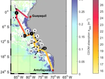
Figure 1.Cruise track of ASTRA-OMZ with stations 1–18 (in black circles: stations where OCS profiles were taken). The cruise track shows sea surface temperature (SST) measured onboard. For visu- alization only, the background is composed of MODIS Aqua satel- lite data for the absorption of CDOM and detritus corrected from 443 to 350 nm with the mean slope of our in situ measurements (0.0179, 300–450 nm; MODIS Aqua composite for October 2015).

Note: as a monthly composite does not necessarily reflect the exact conditions during the cruise, in situ measurements are illustrated in Fig. 2e. White areas: no satellite data available.

2 Material and methods 2.1 Study area

The cruise ASTRA-OMZ on RVSonnestarted in Guayaquil, Ecuador, on 5 October 2015 and reached Antofagasta on 22 October 2015 (Fig. 1). It covered several regimes from the open ocean to the coastal shelf between 5^◦N and 17^◦S.

The hydrographic conditions encountered during this cruise have been described elsewhere (Stramma et al., 2016). The area off Peru is associated with one of the four major global eastern boundary upwelling systems (Chavez et al., 2008). A large oxygen minimum zone expands into the Pacific Ocean at depths between 100 and 900 m, resulting from weak ven- tilation and strong respiration (Karstensen et al., 2008). The cruise covered areas of open ocean with warm sea surface temperatures (SSTs) between 22 and 27^◦C (stations 1–6) and regions with colder SSTs below 20^◦C closer to the coast (sta- tions 7–18). Upwelling occurred at the southernmost tran- sects indicated by the lowest SSTs (15–18^◦C) encountered during that cruise (stations 15–18).

2.2 Measurement of trace gases

Carbonyl sulfide concentrations were determined with an off-axis integrated cavity output spectrometer (OA-ICOS;

Los Gatos Inc., USA) coupled to a Weiss-type equilibrator (Lennartz et al., 2017). The Weiss-type equilibrator was sup-

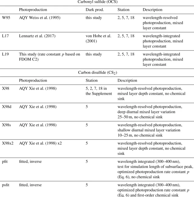
Table 1.Model experiments with 1-D GOTM–FABM modules for OCS and CS₂. AQY: apparent quantum yield.

Carbonyl sulfide (OCS)

Photoproduction Dark prod. Station Description

W95 AQY Weiss et al. (1995) this study 2, 5, 7, 18 wavelength-resolved photoproduction, mixed layer constant

L17 Lennartz et al. (2017) von Hobe et al. 2, 5, 7, 18 wavelength-integrated

(2001) photoproduction, mixed

layer constant L19 This study (rate constantpbased on this study 2, 5, 7, 18 wavelength-integrated

FDOM C2) photoproduction, mixed

layer constant Carbon disulfide (CS₂)

Photoproduction Station Description

X98 AQY Xie et al. (1998) 5, 2, 7, 18 in wavelength-resolved photoproduction, the Supplement mixed layer depth constant, no chemical

sink

X98d AQY Xie et al. (1998) 5 wavelength-resolved photoproduction,

deep diurnal mixed layer variation 25–50 m, no chemical sink

X98s AQY Xie et al. (1998) 5 wavelength-resolved photoproduction,

shallow diurnal mixed layer variation 10–25 m, no chemical sink

X98x2 AQY Xie et al. (1998) x2 5 wavelength-resolved photoproduction, mixed layer depth constant, no chemical sink

pfit fitted, inverse 5 wavelength integrated (300–400 nm),

test for simulation length of subsurface peak, optimized photoproduction rate constantp (Eq. 6), no chemical sink

psfit fitted, inverse 5 wavelength integrated (300–400 nm),

optimized photoproduction rate constantp (Eq. 6) and first-order chemical sink

plied with 2–4 L min⁻¹ of seawater from the hydrographic shaft of the ship 5 m below the surface. The sample gas stream from the headspace of the equilibrator was filtered (Pall Acro Filter, 0.2 µm) and dried (Nafion^®drier, Gasmet Perma Pure) before entering the cavity of the OCS analyzer.

The outlet of the OCS analyzer was connected to the Weiss equilibrator, as this recirculation method kept the concentra- tion gradient between the water and gas phases small, en- abling rapid equilibration. OCS calibrations using standards from permeation tubes (Fine Metrology, Italy) were per- formed before and after the cruise, showing good agreement.

Details on the OA-ICOS can be found in Schrade (2011).

The precision of this setup is 15 ppt for 2 min averages of 1 Hz measurement frequency and was experimentally deter- mined (running a standard for>60 min). The limit of detec-

tion is 180 ppt (corresponding to 4 pmol L⁻¹ at 20^◦C), de- fined by the instrument’s internal 1 s spectra. Additionally, independent samples for comparison measured with GC-MS (Schauffler et al., 1998; de Gouw et al., 2009) reflected a

<2 % difference between the NOAA scale (Montzka et al., 2007) and the perm tube standards. A corrected calibration led to a minor change in absolute concentrations of OCS compared to Lennartz et al. (2017), which was on average +2 pmol L⁻¹. Marine boundary layer air was measured ev- ery hour for 10 min by pumping air from the ship’s deck (ca.

35 m a.s.l.) through a metal tube (Decabon) with a chemi- cally inert pump (KNF Neuberger). Resulting emissions are reported in Lennartz et al. (2017).

OCS depth profiles were obtained using a newly devel- oped submersible pumping system. A rotary pump (Lowara,

Xylem) connected to a 1” PTFE hose supplied the Weiss equilibrator with 2–4 L seawater min⁻¹. The pump inlet was held at a constant depth for 10–15 min to ensure full equili- bration at four to six depths during each profile.

CS₂was measured with a purge-and-trap system attached to a gas chromatograph and mass spectrometer (GC–MS;

Agilent 7890A, Agilent 5975C; inert XL MSD with triple axis detector) running in single-ion mode (Lennartz et al., 2017); 50 mL samples were taken in 1 to 3 h intervals from the same underway system as for continuous OCS measure- ments. After purging for 15 min with helium (70 mL min⁻¹), the gas stream was dried with a Nafion^® membrane drier (Gasmet Perma Pure) and trapped with liquid nitrogen for preconcentration. Hot water was used to heat the trap and inject CS2 into the GC–MS. The retention time for CS2

(^m_z =76, 78) was 4.9 min. The analyzed data were calibrated daily using gravimetrically prepared liquid CS₂standards in ethylene glycol. During purging, 500 µL gaseous deuterated dimethyl sulfide (d3-DMS) and isoprene (d5-isoprene) were added to each sample as an internal standard to account for possible sensitivity drift between calibrations. The limit of detection was 1 pmol L⁻¹. Discrete samples from depth pro- files were obtained from the rosette sampler connected to a conductivity–temperature–depth (CTD) sensor. Note that OCS and CS₂ profiles were not obtained at the same time but up to 7 h apart. The stations were defined by geograph- ical location and not by a Lagrangian experiment following the same water mass, which explains temperature changes between OCS and CS2profiles, for example at station 2 (see Fig. 2c, Table S2).

2.3 Chromophoric dissolved organic matter (CDOM) The spectral absorption coefficient of CDOM (a₃₅₀) was de- termined for samples collected from CTD Niskin bottles or from the underway system, here in a 3 h interval. The sampled water was filtered through a sample-washed 0.2 µm membrane (GWSP, Millipore) after prefiltration through a combusted glass-fiber filter (GFF, Whatman). The optical density of the CDOM in the filtrate was analyzed using a spectrophotometric setup with a liquid waveguide capillary cell (LWCC, WPI; path length: 2.5 m) (Miller et al., 2002).

Spectra were recorded for wavelengths between 270 and 700 nm at 2 nm spectral resolution for the sample filtrate and purified water as the reference, with the sample and refer- ence at room temperature. The absorption coefficient is deter- mined from the obtained optical density using the Lambert–

Beer law and corrected for the salinity effect (see Lefering et al., 2017, for details).

2.4 Fluorescent dissolved organic matter (FDOM) Fluorescent dissolved organic matter (FDOM) was recorded in excitation–emission matrices (EEMs) with a UV–Vis spec- trofluorometer (Hitachi F2700) from filtered seawater sam-

ples (0.2 µm, <200 mbar below atmospheric pressure) di- rectly onboard. Excitation wavelengths ranged from 220 to 550 nm with a resolution of 10 nm. Emission wavelengths were recorded from 250 to 550 nm in 1 nm resolution at a photomultiplier voltage of 400 or 800 V due to a change in method during the campaign (from 10 October 2015 on- wards). For both voltages, calibration curves with quinine sulfate (5 to 30 ppb) in sulfuric acid were measured withR² of 0.9991 and 0.9971, respectively. EEMs were blank sub- tracted and Raman normalized (Murphy et al., 2013). The values are reported here in quinine sulfate units (QSUs). A parallel factor analysis (PARAFAC) was performed using the drEEM toolbox (Murphy et al., 2013; Stedmon and Bro, 2008) to separate the superimposed optical signals of differ- ent fluorophores (“components”) in the EEMs. FDOM con- centrations are reported here in quinine sulfate units (Mur- phy et al., 2013); the conversion factor between QSUs and Raman units is 0.3540 and 0.4256 for each of the QS cali- brations (i.e., before and after the change in photomultiplier voltage, respectively). The components were compared to the database OpenFluor (Murphy et al., 2014) to identify similar components from previous studies in other environments.

2.5 Solid-phase extractable dissolved organic sulfur (DOS_SPE)

DOSSPE was sampled from the underway system or from submersible pump profiles directly into glass bottles and fil- tered through precombusted GF/F filters (Whatman, 450^◦C for >5 h) at a maximum of 200 mbar below atmospheric pressure; 450 mL of each filtered sample was acidified to pH 2 (hydrochloric acid, Suprapur; Merck), extracted accord- ing to Dittmar et al. (2008) (PPL, 1 g, Mega Bond Elut; Var- ian), and stored at−20^◦C until further analysis. For analy- sis, the PPL cartridges were eluted with 5 mL of methanol (LiChrosolv, Merck). DOS_SPEwas quantified with an induc- tively coupled plasma–optical emission spectrometer (ICP- OES; iCAP 7400, Thermo Fisher Scientific), and 100 µL of the extract was evaporated with N₂ and redissolved in 1 mL nitric acid (1 M, double distilled; Merck); 1 mL of yt- trium (2 µg L⁻¹ in the spike solution) was added as an in- ternal standard. The sulfur signal was detected at a wave- length of 182.034 nm. Nitric acid (1 M, double distilled, Merck) was used for an analysis blank. Calibration stan- dards were prepared from a stock solution (1000 mg L⁻¹sul- fur ICP standard solution; Carl Roth). To assess the accuracy and precision of the method, the SLRS-5 reference standard was analyzed five times during the run. Although sulfur is not certified for SLRS-5, a previous study (Yeghicheyan et al., 2013) reported S concentrations of 2347–2428 µg S L⁻¹, which is in agreement with our findings. The limit of detec- tion (according to German industry standard DIN 32645) was 1.36 µmol L⁻¹S, corresponding to 0.015 µmol L⁻¹DOS_SPE in original seawater (average enrichment factor of 89.4).

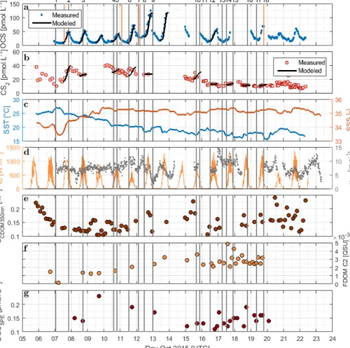
Figure 2.Time series of(a)OCS,(b)CS₂,(c)SST and sea surface salinity (SSS),(d)I0 and wind speed at 10 m,(e)absorption coefficient of CDOM at 350 nm,(f)humic-like FDOM component 2, and(g)DOS_SPEsampled from the underway system along the cruise track of ASTRA-OMZ from 5 to 23 October 2018. Vertical lines indicate stations of ASTRA-OMZ for comparison with locations (see Fig. 1).

2.6 Shortwave radiation in the water column

Underwater shortwave radiation was assessed through down- welling irradiance profiles obtained with the hyperspectral radiometer RAMSES ACC-VIS (TriOS GmbH, Germany).

This instrument covers a wavelength range of 318 to 950 nm with an optical resolution of 3.3 nm and a spectral accuracy of 0.3 nm. Measurements were collected with sensor-specific automatically adjusted integration times (between 4 ms and 8 s). Radiometric profiles were collected down to the max- imum at which light could be recorded prior to or after CDOM–FDOM sampling except at station 7 where sampling took place at night only. Shortwave radiation was approxi- mated at this station with the shortwave radiation profile at station 6, which had similar properties in chlorophylladis- tribution in the water column.

Following NASA protocols (Mueller et al., 2003), all downwelling irradiance profiles were corrected for incident sunlight (e.g., changing due to varying cloud cover) using si- multaneously obtained downwelling irradiance at the respec- tive wavelength, measured above the surface with another

hyperspectral RAMSES irradiance sensor. Finally, these data were interpolated on discrete intervals of 1 m.

As surface waves strongly affect measurements in the up- per few meters, deeper measurements that are more reliable can be further extrapolated to the sea surface. Each profile was checked and an appropriate depth interval was defined (ranging 4–25 for station 2 and 2–25 m for the other three stations) to calculate the vertical attenuation coefficients for downwelling irradiance (i.e., K_d(λ,z’)) for the upper sur- face layer. WithK_d(λ,z’) the subsurface irradianceE_d⁻(λ, 0 m) was extrapolated from the profiles ofE_d(λ,z) within the respective depth interval. Finally, shortwave radiation rad(z) and photosynthetically active radiation PAR(z) were calcu- lated as the integral overE_d⁻(λ, z) for λ=318 to 398 nm and forλ=400 to 700 nm, respectively, for the depths above the lower limit of the respective depth interval and the orig- inally measuredE_d⁻(λ,z) for the depths below. Finally, the euphotic depthZ_euat each station was calculated from the in situ PAR profiles as the 1 % light depth at which PAR(z) 0.01 of PAR(z=0 m).

2.7 Determination of gas diffusivity with microstructure profiles

Diapycnal diffusive gas fluxes, i.e., fluxes of dissolved gas compounds caused by turbulent mixing in a direction per- pendicular to the stratification, were calculated for the four stations 2, 5, 7, and 18. The diapycnal diffusive flux of a compound,ϕ_dia(pmol m⁻²s⁻¹), is estimated as

8_dia≈ρ·K_ρ·∂c

∂z, (1)

where^∂c_∂z(pmol kg⁻¹m⁻¹) is the vertical gradient of gas con- centration across a layer of ideally constant stratification and constant diffusivity, Kρ (m²s⁻¹) is the diapycnal turbulent diffusivity, andρ(kg m⁻³) is the water density. Fluxes can be estimated for depth ranges that are limited above and below by concentration measurements and that do not vary system- atically in stratification and turbulent mixing within. Partic- ular focus is on fluxes to and from the mixed layer (ML), which cause particular issues because of the sudden changes in stratification and mixing intensity at the mixed layer depth (MLD). That is why we approximate ML fluxes by fluxes through a transition zone at 5 to 15 m below the MLD, fol- lowing Hummels et al. (2013), because stratification there is typically strong and relatively constant. MLD was defined here as the depth at which the density has increased by an amount equivalent to a 0.5 K temperature decrease compared to the surface (Schlundt et al., 2014). The diapycnal turbu- lent diffusivityKρ was estimated from the average dissipa- tion rate of turbulent kinetic energy, which in turn was esti- mated from profiles of velocity microstructure. Details on the methodology to estimate the diapycnal fluxes of dissolved substances from microstructure measurements and concen- tration profiles can be found in Fischer et al. (2013) and Schlundt et al. (2014). The microstructure profiles were ob- tained with a tethered profiler (type MSS 90D, Sea & Sun Technology).

The depths at which fluxes could be estimated were then used as the upper and lower bounds of budget volumes. The difference of the diapycnal fluxes in and out of each vol- ume determines convergence or divergence of the diapycnal flux. If other transport processes are negligible and if steady state is assumed, sources–sinks to compensate for the flux divergence–convergence can be determined.

Uncertainties of fluxes have been calculated by error prop- agation from measurement uncertainties of the gas concen- trations and the averageK_ρ values. There are additional un- certainties not quantified, e.g., from the approximation of the average gas gradient or from the neglect of gas transport pro- cesses other than diapycnal mixing. It should be noted that the diffusivity profile only represents current conditions dur- ing profiling and can change on a daily basis due to varying stratification and/or surface winds among other factors.

2.8 Determination of OCS dark production rates Dark production rates were determined from hourly aver- aged measured seawater concentrations shortly before sun- rise (i.e., ca. 12–14 h after the concentration maximum of the previous day) or at depths below the euphotic zone. Con- centration data from this study and a previous study from the Indian Ocean (Lennartz et al., 2017) were used to cal- culate dark production rates. The determination of dark pro- duction rates relies on the principle that in the absence of light, an equilibrium between dark production and loss by hydrolysis results in stable concentrations (Von Hobe et al., 2001). To ensure approximately steady-state conditions, we averaged the concentrations 1 h before sunrise and compared to the average of the previous hour. We only considered in- stances when the concentration before sunrise deviated less than 1 pmol L⁻¹from the previous hour for further calcula- tion. These conditions were met at the beginning of the cruise (7 to 12 October), when water temperatures ranged between 21 and 26^◦C and the correspondinge-folding lifetimes of OCS due to hydrolysis ranged from 6 h (7 October) to 12 h (12 October). In steady state (early morning or below the eu- photic zone), dark productionPD(pmol L⁻¹s⁻¹) equals loss by hydrolysisLH (pmol L⁻¹s⁻¹), the latter being the prod- uct of the steady-state concentration (OCS; pmol L⁻¹) and the rate constant k_h(s⁻¹) according to Eq. (2):

PD=LH= [OCS] ·k_h. (2) The rate constant for hydrolysis, kh(s⁻¹), was calculated ac- cording to Elliott et al. (1989) with Eqs. (3) and (4):

kh=e^{(24.3−10450T )}+e^{(22.8−6040T )}· K_w

a[H⁺], (3)

−log₁₀K_w=3046.7

T +3.7685+0.0035486·

√

S, (4)

with temperatureT, salinityS, a[H]⁺ the proton activity, andK_w the ion product of seawater (Dickinson and Riley, 1979).

The temperature dependency of the reaction rate P_D (pmol L⁻¹s⁻¹) can be described with an Arrhenius relation- ship, resulting in the following equation (Eq. 5) in its lin- earized form:

ln P_D

a₃₅₀

= a

T +b, (5)

with a350 being the absorption coefficient of CDOM at 350 nm (m⁻¹),T the temperature (K), and a andb coeffi- cients describing the temperature dependency of the reaction (–). The production rateP_Dis normalized toa₃₅₀(von Hobe et al., 2001). The parametersaandbin Eq. (5) were derived fromP_D(Eq. 5) in the Arrhenius plot to obtain a parameteri- zation for dark production rate in relation to temperature and a₃₅₀.

Biases can potentially be introduced in two ways: (1) ne- glecting other sinks like air–sea exchange can lead to un- derestimations of the production rate. With wind speeds of 8 m s⁻¹ and MLD on the order of 20–40 m, lifetimes due to air–sea exchange are on the order of days to weeks and hence negligible. (2) Sampling fewer than two half-lives after the maximum concentrations can lead to overestimations of the production rate. For 11 and 12 October, samples consid- ered for the calculation of dark production rates were taken fewer than two half-lives after the concentration maximum of the previous day. Since the concentration changed less than 1 pmol L⁻¹within 2 h prior to this sampling, we consider the bias to be within the range of the given uncertainty.

2.9 Surface box models to estimate photoproduction rate constants

The surface box model for OCS has already been used in Lennartz et al. (2017) to estimate OCS photoproduction rate constants. The model consists of parameterizations for the four processes of hydrolysis (Elliott et al., 1989), dark pro- duction (Von Hobe et al., 2001), photoproduction (Lennartz et al., 2017), and air–sea exchange (Nightingale et al., 2000).

In situ measurements of meteorological, physical, and bio- geochemical parameters are used as model forcing. Photo- chemical production was calculated according to Eq. (6):

dcphoto

dt =

0

Z

MLD

UV·a350·p, (6)

with ^dcphoto_dt being the change in concentration due to pho- toproduction (pmol L⁻¹s⁻¹), UV the irradiance in the UV range (W m⁻²), a350 the absorption coefficient of CDOM at 350 nm (m⁻¹), andp the photoproduction rate constant (pmol J⁻¹). The model was set up in an inverse mode con- strained by time series of OCS measurements

dc dt

to op- timize the photoproduction rate constant p during each daylight period (13:00 to 23:00 h UTC) with a Levenberg–

Marquardt routine (MATLAB version 2015a, MathWorks, Inc.). The scaling of the rate constantp can be seen as the contribution of the precursors varying in concentration, as detailed in von Hobe et al. (2003).

An analogous model setup was developed for CS₂, includ- ing only the processes of air–sea exchange and photopro- duction. The estimated production rate hence compensates for the sink of air–sea exchange. Processes without known parameterizations, such as possible biotic production and a potential (chemical) sink, are excluded at this stage (see the Discussion section). More information on the model forcing parameters can be found in the Supplement (Tables S1 and S2).

2.10 1-D water column modules for OCS and CS₂ The Framework for Aqueous Biogeochemical Modelling (FABM) was used to couple the box model to a 1-D water column model (Bruggeman and Bolding, 2014) and com- pare simulated concentrations to observations at stations 2, 5, 7, and 18. FABM provides the frame for a physical host model and a biogeochemical model, wherein the physical host is responsible for tracer transport and the biogeochem- ical model provides local source and sink terms. The phys- ical host used here is the General Ocean Turbulence Model (GOTM), which is a 1-D water column model simulating hy- drodynamic and thermodynamic processes related to vertical mixing (Umlauf and Burchard, 2005). GOTM derives solu- tions for the transport equations of heat, salt, and momentum.

In situ measurements of radiation, temperature, salinity, CDOM, and meteorological parameters were used as model forcing to represent conditions under which the concentra- tion profiles were taken. Diurnal radiation cycles and con- stant meteorological conditions, salinity, and water temper- ature were repeated for 5 d for OCS to obtain stable diurnal concentration cycles and 21 d for CS₂due to its longer life- time.

The same process parameterizations as for the box models were used as local source and sink terms in the 1-D water column modules for OCS and CS₂in FABM. Photochemi- cal production was calculated in the wavelength-integrated approach (300–400 nm) described above in Eq. (6) and, in addition, in a wavelength-resolved approach. For this pur- pose, we used in situ measured, wavelength-resolved down- welling irradiance profiles together with in situ wavelength- resolved CDOM absorption coefficients to model the photo- production of both gases in the water column based on previ- ously published apparent quantum yields (AQYs) by Weiss et al. (1995) for OCS and by Xie et al. (1998) for CS₂. We use the AQYs by Weiss et al., since they were measured at the location closest to our study region (i.e., South Pacific).

We assume they reflect the DOM composition in our study region best due to their similarity ina₃₅₀. We note other ob- served AQYs (Zepp and Andreae, 1994; Cutter et al., 2004), which vary by up to 2 orders of magnitude. In addition, the photoproduction rate constantpof OCS in Eq. (6) was cal- culated based on the relationship with FDOM component 2 developed in this study.

In addition, sensitivity tests were performed to further con- strain production and consumption processes for CS2. Here we assessed the sensitivity of the general shape of the pro- files and did not focus on exact production rates, since both sink and source processes are too poorly constrained to de- rive reaction rates from single concentration profiles. Pro- files were initialized with the lowest subsurface concentra- tion of the respective measured profile: low enough to be able to assess whether in situ photoproduction can explain concentration peaks below the mixed layer, but high enough to keep diapycnal fluxes out of the mixed layer in a reason-

able range (in contrast to initializing with 0 pmol L⁻¹). The same meteorological conditions that occurred on the day of measurement were repeated for 21 d, i.e.,∼2–3 times longer than the lifetime due to air–sea exchange. These sensitiv- ity tests demonstrate (1) the sensitivity of surface CS₂con- centrations against diurnal mixed layer variations (simula- tions X98, X98d, X98s) and (2) the sensitivity of the sub- surface CS₂peak against the photoproduction rate constant and wavelength resolution (simulations X98x2, pfit, psfit).

Testing the sensitivity against diurnal mixed layer variations is important because surface CS₂concentrations depend on the amount of photochemical production occurring within the mixed layer. Air–sea exchange as the major sink for CS2

within the mixed layer led to relatively long lifetimes on the order of days to weeks during this cruise, so the conditions during the days prior to the CS2 profile measurements be- came important. Simulations with adjusted temperature and salinity profiles with a diurnally varying mixed layer be- tween 10–25 m (“shallow” simulation X98s) and 25–50 m (“deep” simulation X98d) were performed. For the second test, demonstrating the sensitivity of the subsurface peak, we chose station 5. This station provides the unique opportunity to assess a profile in which the photic zone reaches below the ML; hence, photoproduction might occur at depths at which the sink of air–sea exchange is absent due to the bottom of the mixed layer acting as a barrier. We used two scenarios to assess the subsurface concentrations with one photopro- duction rate constantpacross the profile, which is consistent with surface concentrations: (1) a scenario during which the AQY by Xie et al. (1998) is scaled by a factor of 2 to match the surface concentration in a wavelength-resolved approach and (2) a scenario in which p is fitted with a wavelength- integrated approach (Eq. 6) with (simulation psfit) and with- out (simulation pfit) allowing for an additional chemical first- order sink.

An overview of the model experiments is listed in Table 1, and more information on the model forcing and setup can be found in the Supplement (Table S2).

3 Results

3.1 CDOM, FDOM, and DOSSPE

DOM showed strong spatial variability in FDOM but less in the DOSSPEconcentration and CDOM absorbance. CDOM, here shown as the absorption coefficient at 350 nm, was on average a350=0.15±0.03 m⁻¹ (coefficient of varia- tion – CV: 0.2 m⁻¹). The highest absorption coefficients were found closest to the continent and in the upwelling- influenced region between 17 and 20^◦S (Fig. 2e), as expected in upwelling regions (Nelson and Siegel, 2013). This spatial pattern was consistent with the monthly composite of satel- lite data (Fig. 1).

Four different components of FDOM, representing groups of similarly fluorescing molecules, were isolated and val- idated with PARAFAC analysis. Components C1 (aver- age±standard deviation 0.015±0.0119 QSU, CV: 0.79) and C4 (0.0091±0.0158 QSU, CV: 1.74) have their fluores- cence peak in the UV part of the EEM (see the Supple- ment, Fig. S1). They resemble the naturally occurring amino acids tryptophane and tyrosine (Coble, 2007). Components C2 (0.0032±0.0027 QSU, CV: 0.84) and C3 (0.0032± 0.0158 QSU, CV: 0.91) fluoresce in the visible range (Vis- FDOM) of the EEM. Their fluorescence pattern showed char- acteristics of humic-like substances and they were abundant, especially in the southern part of the cruise closer to the con- tinent and upwelling region (C2 in Figs. 2f and S1).

Surface DOSSPEonly showed minor variations along the cruise track with concentrations of 0.16±0.05 µmol L⁻¹ (CV: 0.31). The highest surface DOS_SPEconcentrations were found in the 16^◦S transect connected to an active upwelling cell and in the open-ocean part of the cruise (Fig. 2g).

DOS_SPE concentrations in the water column (not shown) decreased with depth, as also found in the eastern Atlantic Ocean and the Sargasso Sea (Ksionzek et al., 2016). Concen- trations decreased from 0.76 (5 m depth) to 0.33 µmol L⁻¹ in 100 m at station 7, from 0.62 (25 m) to 0.49 µmol L⁻¹ (125 m) at station 7, and from 0.49 (20 m) to 0.28 µmol L⁻¹ (115 m) at station 18. At station 2, concentrations of 0.89–

0.91 µmol L⁻¹ were measured at a depth of 50–100 m; no surface data are available.

3.2 Carbonyl sulfide (OCS)

3.2.1 Horizontal and vertical distribution

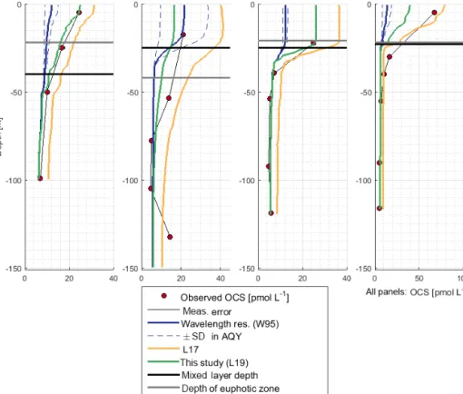
OCS surface water concentrations ranged from 6.4 to 144.1 pmol L⁻¹(average 30.5 pmol L⁻¹) with strong diurnal cycles as described in Lennartz et al. (2017). Surface con- centrations increased towards the shelf and coast, were the highest along a shelf transect from 8 to 12^◦S, and were con- nected to a fresh upwelling patch around 16^◦S (Fig. 2a). Sur- face concentrations and emissions to the atmosphere are de- scribed in detail in Lennartz et al. (2017). The concentra- tions in the water column decreased with depth at stations 2, 7, and 18 to ca. 10 pmol L⁻¹ below the euphotic zone with varying gradients. Profiles at stations 7 and 18 ranged down to the oxygen minimum zone, but the concentration profiles did not show any corresponding discontinuity. The shape of the concentration profile for station 5 differed from the other stations: here the profile had a convex shape down to 75 m, and it was the only station where a subsurface concentration peak was recorded at a depth of 136 m (Fig. 3).

3.2.2 Dark production

The dark production rates at the surface varied between 0.86 and 1.81 pmol L⁻¹h⁻¹along the northern part of the cruise

Figure 3.Profile measurements of OCS concentrations and 1-D model results for the OCS model experiments described in Table 1.

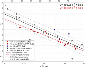
track and between 0.16 and 0.81 pmol L⁻¹h⁻¹ in the four depth profiles below 50 m. The Arrhenius-type temperature dependency showed significantly increasing dark production rates with increasing temperature (Pearson’s test,p=5.66× 10⁻¹⁰). Dark productionPDat both the surface and at depth along the cruise track (Fig. 4) is described by the following Arrhenius equation:

P_D=a₃₅₀·exp

−15182 T +53.1

. (7)

The Arrhenius fit could not be improved using FDOM, DOS_SPE, or O₂ instead of a₃₅₀ (not shown). At station 5, the dark production rates at 50 and 136 m were larger than predicted for the temperature and thea₃₅₀(Fig. 4).

The parameterization for dark production, previously in- cluding only dark production rates from the North Atlantic, Mediterranean, and North Sea (Von Hobe et al., 2001), was updated with the data from the Peruvian upwelling and the Indian Ocean; it yields the following semiempirical equation (Eq. 8) (Fig. 4):

P_D=a₃₅₀·exp

−16692 T +58.5

. (8)

3.2.3 Diapycnal fluxes

The diapycnal fluxes of OCS within the water column were derived from measured concentration and diffusivity pro-

files. OCS produced at the surface was mixed downwards in all four profiles. Diapycnal fluxes out of the mixed layer were always 2 or 3 orders of magnitude smaller than emissions to the atmosphere at stations 2, 5, and 7 with diapycnal fluxes of 8.2×10⁻⁴, 2.4×10⁻⁴, and 3.8× 10⁻³pmol s⁻¹m⁻². An exception is station 18, where di- apycnal fluxes (0.48 pmol s⁻¹m⁻²) were almost half of the air–sea flux (−1.0 pmol s⁻¹m⁻²).

3.2.4 Photoproduction

The photoproduction rate constants according to Eq. (6) were previously derived from a surface box model and have al- ready been discussed in Lennartz et al. (2017). For days with concurrent measurements of FDOM (7, 8, 9, 10, 13, 16 Oc- tober 2015), the correlation between photoproduction rate constant and humic-like FDOM C2 was significant (Pear- son’s test, p=0.014, R²=0.81; Fig. 5a). Measurements of FDOM (anda350) during the period used for optimiza- tion of the photoproduction rate constantp(i.e., daylight pe- riod) were averaged for this correlation. The relationship was quantified by Eq. (9):

p=85.8·[FDOM C2]+828.76, (9)

with the photoproduction rate constantp(pmol J⁻¹) and the concentration of the FDOM component C2 (QSU). The cor- relation witha₃₅₀only explains a variance ofR²=0.01 (n=

Figure 4.Arrhenius plot of dark production rates from ASTRA- OMZ (this study, red and blue markers), data from the Indian Ocean (OASIS cruise; Lennartz et al., 2017), and previously published rates (von Hobe et al., 2001; grey markers; note thatPDwas con- verted from original units of pmol m⁻³s⁻¹to pmol L⁻¹h⁻¹; for reconversion subtract 1.28). The red linear fit and equation show the parameterization for ASTRA-OMZ only, whereas the black fit and equation represent an updated parameterization including dark production rates from this and previous studies (see Von Hobe et al., 2001).

7, i.e., 7, 8, 9, 10, 12, 13, 16 October 2015).R²increases to 0.3 when the respective days for FDOM C2 correlations are considered (p>0.25). C2 anda350were not significantly cor- related during these days (p>0.2,R²=0.36) but showed a similar spatial trend over the entire cruise track (Fig. 2). Al- though our experiment was not strictly Lagrangian,a₃₅₀only changed<0.05 m⁻¹within each respective fitting period. For FDOM C2, only one to two measurements per daylight pe- riod were available during the days when photoproduction rate constants were fitted, but variations of only 0.003 QSU per day were encountered during high-frequency sampling towards the end of the cruise. This relationship thus carries some uncertainties and will benefit from additional data from other regions.

OCS concentrations in the water column were simulated with the new module in the model environment of GOTM–

FABM. While the AQY of Weiss et al. (1995) yielded sur- face concentrations a factor of 3–6 too small compared to ob- servations, the L17 simulation overestimated concentrations in all cases up to twofold (Fig. 3). Deviations between sim- ulations and measurements were reduced by using the up- dated dark production rate of this study and the linear cor- relation between FDOM C2 and p shown in Fig. 5a (Eq. 9;

see Sect. 3.2.2). At station 18, surface concentrations were simulated lower than observed. The shapes of the concen- tration profiles were well reflected in the simulations ex-

Figure 5.Correlations of the photoproduction rate constant from inverse surface box modeling for(a)OCS and FDOM component C2 as well as(b)CS₂and DOS_SPE.

cept at station 5, where the subsurface concentration peaks at 55 and 136 m were not adequately reproduced. Despite the different magnitude of the wavelength-resolved (W95) and wavelength-integrated (L17, L19) approaches, the shape of the photoproduction profile in the water column did not show major differences.

3.3 Carbon disulfide (CS2)

3.3.1 Horizontal and vertical distribution

The surface concentration of CS2during ASTRA-OMZ was in the lower picomolar range, with an average of 17.8± 8.9 pmol L⁻¹, and displayed diurnal cycles only on some days (e.g., 7 October 2015) but not on the majority (Fig. 3).

The spatial pattern of sea surface concentrations was oppo- site to that of OCS, with the highest concentrations distant from the shelf and the lowest closer to the shore. The high- est surface concentrations of CS₂coincided with warm tem- peratures (Fig. 2b and c). Surface temperatures T (^◦) and concentrations of CS₂(pmol L⁻¹) were binned for daily av- erages and yielded the following relationship (p=0.0026, R²=0.61) of (Eq. 10):

[CS₂]=2.3T−27.2. (10)

The concentration profiles of CS2 did not show a steep de- crease with depth like OCS, but they were more homoge- neous (Fig. 6) apart from subsurface peaks below the mixed layer that occurred, for example, at stations 2, 5, and 18.

The concentration in CS₂profiles down to about 200 m was distinctly higher in profiles on which upwelling did not oc- cur (stations 1 to 13;∼20 pmol L⁻¹) compared to stations in the southern part of the cruise track (stations 15 to 18;

∼10 pmol L⁻¹). This difference in concentrations through- out the water column reflected the pattern observed at the surface, where high concentrations coincide with high tem- peratures.

Figure 6.Concentration depth profiles for discrete measurements of CS₂ for open-ocean regions (stations 1–5, blueish colors) and stations closer to the shelf (stations 6–13, green–yellow colors).

3.3.2 Diapycnal fluxes

The diapycnal fluxes of CS₂ within the water column re- vealed the highest production at the surface except for station 18. Within the water column, CS₂was redistributed down- wards. Small in situ sinks (stations 2, 7, and 18) and in situ sources at different water depths (stations 2 and 18) within the water column were required to maintain convergences–

divergences under a steady-state assumption. Fluxes out of the ML were 7.6×10⁻⁴, 3.3×10⁻⁴, 1.9×10⁻³, and 0.98 pmol s⁻¹m⁻² at stations 2, 5, 7, and 18 and thus 1–3 orders of magnitude smaller than fluxes to the atmosphere.

At station 18, diapycnal fluxes out of the ML and emissions to the atmosphere were at a similar magnitude (0.98 and

−1.0 pmol s⁻¹m⁻², respectively).

3.3.3 Photoproduction of CS₂

Photoproduction rate constants for CS₂were determined us- ing an inverse setup of the surface box model analogous to OCS, but including only photoproduction and air–sea ex- change as source and sink terms. The resulting photoproduc- tion rate constants were between 5 and 70 times smaller than those of OCS. Opposite to OCS, the rate constants did not co- vary significantly with any FDOM component (p0.05). A weak trend was detected for DOS_SPE(p=0.08, Spearman’s

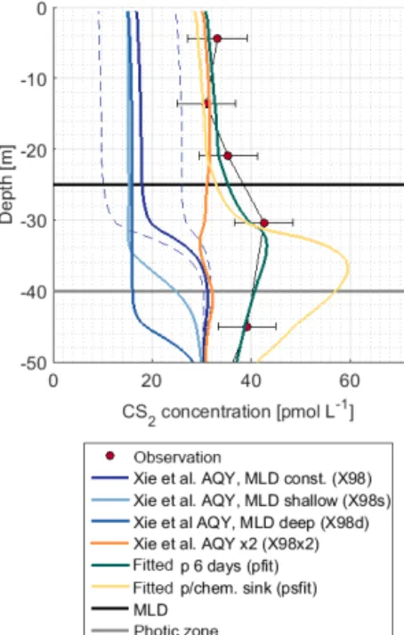
Figure 7.Observation and model sensitivity simulations at station 5. AQY: apparent quantum yield, MLD: mixed layer depth. Simu- lation names in brackets refer to Table 1. Dashed lines indicate the confidence interval of AQY as reported in Xie et al. (1998).

r²=0.44,n=8; Fig. 5), and all other tested parameters did not show any correlation (FDOM C1-C4, CDOM).

The shape of the CS2concentration profiles was modeled for four stations (Fig. S2) with the scenarios described in Ta- ble 1. Concentrations in the mixed layer of stations 2, 5, and 7 using the wavelength-resolved AQY from Xie et al. (1998) yielded concentrations 4–6 times lower than observed (sim- ulation X98).

The influence of mixed layer depth variations was tested in simulations X98d and X98s. Surface concentrations dif- fered from the reference simulation X98 by<2.5 pmol L⁻¹ (Fig. 7). The shape of the concentration profile, however, was sensitive to mixed layer variations, as indicated by the sensi- tivity simulations X98d and X98s. In these artificially created test scenarios, concentrations accumulated below the bottom of the deepest mixed layer during the simulation period.

The subsurface concentration peak was investigated with (1) simulation X98x2, with the wavelength-dependent AQY by Xie et al. (1998) scaled by a factor of 2 so that it matches CS₂ concentrations in the mixed layer, and (2) simulations pfit and psfit in which a photoproduction rate constant in an integrated wavelength approach (Eq. 6) was fitted to ob- served profiles (corresponding to an evenly distributed AQY across wavelengths of 300–400 nm). Simulation X98x2 does not reproduce the subsurface peak, whereas simulations pfit and psfit are two possible scenarios to reproduce the observed peak (Fig. 7). Photoproduction rates for these simulations are shown in Fig. S3.

Figure 8. (a)Rate of sulfide production due to OCS hydrolysis as a function of temperature and OCS concentration, calculated with Eqs. (3) and (4).(b)Average consumption of S (organic or inorganic sulfide) by OCS photoproduction and the production of sulfide dur- ing hydrolysis from ASTRA-OMZ (average for 7–14 October).

4 Discussion 4.1 Carbonyl sulfide

The four profiles at stations 2, 5, 7, and 18 represent the first observations of OCS profiles in the upwelling area off Peru. They do not indicate any connection to a significant redox-sensitive process, as most profiles show a continuous decreasing shape as expected for photochemically produced compounds with a short lifetime in seawater. The indepen- dence from dissolved oxygen concentrations is in line with previous findings (Zepp and Andreae, 1994; Uher and An- dreae, 1997). Station 5 was the only profile that differed in shape. This profile was measured in an eddy in which down- ward mixing occurred (Stramma et al., 2016), which may ex- plain the increased concentrations at 55 m. Profiles at station 7 and 18 reached down to the sediment but did not show in- creased concentrations towards the bottom. Increased sedi- ment inputs, as reported, e.g., from estuarine regions (Zhang et al., 1998), apparently do not play a large role in the studied region, and fluxes to the atmosphere are not affected.

The study by Zhang et al. (1998) also raises the question of near-surface gradients, suggesting that our shallowest mea- surement depth of 5 m in both profile and underway sampling might underestimate the flux of OCS. On the other hand, strong near-surface stratification acts as a barrier for air–sea exchange (Fischer et al., 2019) and could lead to a bias of the OCS flux if the sampling depth is below the barrier. Since it is difficult to perform underway sampling at depths shal- lower than a few meters, we cannot fully resolve this issue.

However, given the lowa350compared to coastal and estuary regions as in Zhang et al. (1998), irradiation likely penetrates deeper into the water column in our study region than in the estuary in their study. Hence, photochemical production likely extended further down into the water column, which reduces the problem of underestimating the flux.

Dark production rates of up to 1.81 pmol L⁻¹h⁻¹in our study were at the upper end of the range of previously re- ported rates in the open ocean (Von Hobe et al., 2001; Ul- shöfer et al., 1996; Flöck and Andreae, 1996; Von Hobe et al.,

1999) but similar to those from the Mauritanian upwelling region (Von Hobe et al., 1999). Only incubation experiments in the Sargasso Sea showed higher production rates than re- ported here, ranging between 4 and 7 pmol L⁻¹h⁻¹(Cutter et al., 2004). Cutter et al. (2004) concluded that particulate or- ganic matter heavily influences dark production. Although no sample-to-sample comparison to particulate organic carbon (POC) is possible for our OCS data, the general range of POC during our cruise was 12.1±6.1 µmol L⁻¹ (145.2 µg L⁻¹), which is much higher than the POC (ca. 41 µg L⁻¹) reported from the Sargasso Sea (Cutter et al., 2004). We thus cannot confirm the influence of POC on dark production in the Pe- ruvian upwelling and do not find a direct biotic influence.

Our results together with previous studies show that trop- ical upwelling areas are globally important regions for OCS dark production, likely due to the combination of higha350

and moderate temperatures (15–18^◦C). The temperature de- pendency of dark production (Eqs. 7 and 8) is very similar to the one found by Von Hobe et al. (2001) in the North At- lantic, North Sea, and Mediterranean (Fig. 4). The similarity points towards a ubiquitous process across different biogeo- chemical regimes, as the dependence of the production rate on temperature anda₃₅₀ is very similar for an oligotrophic region like the Sargasso Sea (Von Hobe et al., 2001) or the Indian Ocean from the OASIS cruise (Lennartz et al., 2017) and a nutrient-rich and biologically very productive region such as the studied upwelling area. The fit in the Arrhenius dependency could not be improved by parameters other than a350and showed no influence on dissolved O2. The charac- teristics that make a molecule part of the CDOM pool, i.e., unsaturated bonds and nonbonding orbitals, also favor rad- ical formation. OCS dark production is thus best described using abiotic parameters such asa350and temperature rather than biologically sensitive parameters such as dissolved O₂ or apparent oxygen utilization as a proxy for remineraliza- tion. This independence from biotic parameters supports the radical production pathway. The results are in line with find- ings by Pos et al. (1998) showing that these molecules can form radicals in the absence of light, e.g., mediated by metal complexes, and by Kamyshny et al. (2003) showing a pos- itive correlation of dark production rate and temperature.

However, the profile at station 5 provides some evidence that an additional process occurs in the subsurface. The concen- tration peak was visible in the upcast and the downcast, but since we only observed it only once, we cannot conclusively rule out the possibility that the OCS peak at 136 m is an arti- fact. Still, similar subsurface peaks have been reported from stations in the North Atlantic by Cutter et al. (2004). They concluded that dark production is connected to remineraliza- tion.

Diapycnal fluxes at stations 2, 5, 7, and 18 indicate down- ward mixing from the surface to greater depths in all profiles.

However, fluxes were several orders of magnitude smaller than emissions to the atmosphere, except for station 18.

There, high diffusivities were observed using the microstruc-

ture probe, which most likely result from high internal wave activity as indicated by vertical water displacements of up to 30 m during four CTD cases. Diapycnal fluxes will change diurnally with the shape of the concentration profile and mixed layer variations; hence, the measurements here only represent a snapshot. Still, the difference in magnitude be- tween air–sea exchange and diapycnal fluxes seems to be valid at varying times of the day and varying regions in the studied area. Hence, neglecting diapycnal fluxes when calcu- lating OCS concentrations in mixed layer box models leads to only minor overestimations of the concentrations.

An interesting finding is the significant correlation of the photoproduction rate constantpwith FDOM C2 (humic-like FDOM), but not with DOSSPE, given a reported correlation of OCS and DOS in the Sargasso Sea where much higher DOS concentrations of ca. 0.4 µmol S L⁻¹were present (Cut- ter et al., 2004). It should be noted that the method to extract DOS_SPEin our study does not recover all DOS compounds, and we cannot exclude the possibility that this influences the missing correlation between p and DOS. In the studied area, OCS photoproduction is apparently not limited by bulk or- ganic sulfur but rather by humic substances. The humic-like FDOM component C2 is an abundant fluorophore in marine (Catalá et al., 2015; Jørgensen et al., 2011), coastal (Cawley et al., 2012), and freshwater (Osburn et al., 2011) environ- ments. This FDOM component seems to be especially abun- dant in the deep ocean (Catalá et al., 2015), which might be the reason for higher C2 surface concentrations in regions of upwelling, as evident in our study (Fig. 2) and reported by Jørgensen et al. (2011). The significant correlation of p with humic-like fluorophores in our study highlights the impor- tance of upwelling and coastal regions for OCS photopro- duction.

A significant correlation (i.e., a limitation) of OCS pho- toproduction with humic-like substances, but not with bulk DOS_SPE, can be explained by two scenarios: under the as- sumption that only organic sulfur is used to form OCS, the limiting factor is contained in the humic-like C2 fraction of the FDOM pool. The sulfur demand (75.8 pmol L⁻¹; the or- ange area in Fig. 8) would need to be covered entirely by organic, sulfur-containing precursors. The limiting driver of this process is either organic molecules acting as photosen- sitizers or a sulfur-containing fraction of the DOM pool that correlates with FDOM C2 but not bulk DOSSPE. In that sce- nario, FDOM C2 can be used as a proxy for the OCS photo- production rate constant. More data from other regions would help to quantify such a relationship. In a second possible sce- nario under the assumption that both organic and inorganic sulfur can act as a precursor, the sulfur demand could theo- retically be covered by the sulfur generated through the hy- drolysis of OCS (i.e., 85.8 pmol L⁻¹; Fig. 8). In this case, FDOM C2 would only be limiting as long as enough organic or inorganic sulfur is present, for example when temperatures are high enough to recycle sulfur directly from OCS or when other inorganic sulfur sources are present.

Incubation experiments have shown that inorganic sulfur is a precursor for OCS (Pos et al., 1998). It is not clear whether the mechanism proposed in Pos et al. (1998) occurs under en- vironmental conditions because sulfide concentrations were higher than in most marine areas, but also yielded much higher OCS production rates in the magnitude of nM h⁻¹ compared to the magnitude of pM h⁻¹under natural condi- tions. Furthermore, the conversion of sulfide to sulfate, rather than to OCS, is thermodynamically favored. Based on our data, we cannot resolve the question about the role of in- organic sulfur in OCS photoproduction, but our results are consistent with the reaction mechanism suggested by Pos et al. (1998). Incubation experiments at environmentally rele- vant sulfide concentrations, as well as p–DOS relationships across different temperature and DOM regimes, will help to resolve this issue.

Our results show that FDOM C2 is a good candidate as a proxy for OCS photoproduction, but its sampling coverage is insufficient for global model approaches at the moment.

On global scales, on which p varies on a broader range than within the area covered by this study,a₃₅₀ might still be an adequate but not perfect predictor for this variation (Lennartz et al., 2017). On local scales, the parameterization for p based ona₃₅₀can be improved using FDOM C2.

In addition, we used parameterizations from previously re- ported 0-D box models and from this study to assess their ap- plicability to biogeochemical models coupled to a 1-D phys- ical host model. It should be noted, however, that the sur- face data shown here have been used, along with other data, to derive the parameterization for the photoproduction rate constant in Lennartz et al. (2017).

Photoproduction rates based on the wavelength-resolved simulation W95 underestimated observed concentrations in all cases. Other AQYs were not tested but can be interpreted in a relatively straightforward way, since the AQYs of a given spectral shape are proportional to the OCS production and concentration (in steady state). Higher wavelength-resolved AQY as reported by Zepp and Andreae (1994) from the North Sea and the Gulf of Mexico, as well as by Cutter et al. (2004), ranged from twofold to up to 2 orders of mag- nitude higher than the ones reported by Weiss et al. (1995).

These differences in magnitude were attributed to the compo- sition of the DOM pool. To reflect this influence of the DOM composition, Lennartz et al. (2017) parameterized the pho- toproduction rate constant (corresponding to an integrated AQY) to a350, following the suggestion by von Hobe et al. (2003) thata350 can be used as a proxy for OCS precur- sors on larger spatial scales. Using this parameterization for photochemical production in the 1-D water column model (simulation L19) yielded simulated concentrations closer to, but higher than, observations (Fig. 3). Although the absolute concentrations for the AQY W95 did not match observations for the reasons outlined above, the shape of the profile fits the observations well. The simulations thus support the ex- perimental findings in most of the previously published AQY