O production and consumption from stable isotopic and concentration data in the Peruvian

N

₂

O production and consumption from stable isotopic and concentration data in the Peruvian

coastal upwelling system

Annie Bourbonnais¹ , Robert T. Letscher² , Hermann W. Bange³ , Vincent Échevin⁴ , Jennifer Larkum¹, Joachim Mohn⁵ , Naohiro Yoshida^6,7 , and Mark A. Altabet¹

1School for Marine Science and Technology, University of Massachusetts Dartmouth, New Bedford, Massachusetts, USA,

2Earth System Science, University of California, Irvine, California, USA,³GEOMAR, Helmholtz Centre for Ocean Research Kiel, Kiel, Germany,⁴LOCEAN/IRD/IPSL, Laboratoire d’Océanographie et de Climatologie: Expérimentation et Approches Numériques, Paris, France,⁵Empa, Laboratory for Air Pollution and Environmental Technology, Dübendorf, Switzerland,

6Department of Chemical Science and Engineering, Tokyo Institute of Technology, Yokohama, Japan,⁷Earth-Life Science Institute, Tokyo Institute of Technology, Tokyo, Japan

Abstract

The ocean is an important source of nitrous oxide (N₂O) to the atmosphere, yet the factors controlling N₂O production and consumption in oceanic environments are still not understood nor constrained. We measured N₂O concentrations and isotopomer ratios, as well as O₂, nutrient and biogenic N₂concentrations, and the isotopic compositions of nitrate and nitrite at several coastal stations during two cruises off the Peru coast (~5–16°S, 75–81°W) in December 2012 and January 2013. N₂O concentrations varied from below equilibrium values in the oxygen deficient zone (ODZ) to up to 190 nmol L¹ in surface waters. We used a 3-D-reaction-advection-diffusion model to evaluate the rates and modes of N₂O production in oxic waters and rates of N₂O consumption versus production by denitrification in the ODZ. Intramolecular site preference in N₂O isotopomer was relatively low in surface waters (generally3 to 14‰) and together with modeling results, confirmed the dominance of nitrifier-denitrification or incomplete denitrifier-denitrification, corresponding to an efflux of up to 0.6 Tg N yr¹off the Peru coast. Other evidence, e.g., the absence of a relationship betweenΔN₂O and apparent O₂utilization and significant relationships between nitrate, a substrate during denitrification, and N₂O isotopes, suggest that N₂O production by incomplete denitrification or nitrifier-denitrification decoupled from aerobic organic matter remineralization are likely pathways for extreme N₂O

accumulation in newly upwelled surface waters. We observed imbalances between N₂O production and consumption in the ODZ, with the modeled proportion of N₂O consumption relative to production generally increasing with biogenic N₂. However, N₂O production appeared to occur even where there was high N loss at the shallowest stations.

1. Introduction

N₂O is an atmospheric trace gas, mainly produced by microbial processes, that directly and indirectly affects climate. As a tropospheric greenhouse gas, it is ~300 times more potent than CO₂on a per molecule basis [Forster et al., 2007]. With a long atmospheric residence time (>100 years), N₂O produced at the planet’s surface reaches the stratosphere where it acts as the main source of ozone-depleting nitric-oxide radicals [Nevison and Holland, 1997;Ravishankara et al., 2009]. Microbial processes associated with nitrogen cycling are the dominant natural sources of N₂O, with those in the open ocean accounting for up to ~35% of global emissions [Forster et al., 2007; Freing et al., 2012;Ciais et al., 2013]. Still, major uncertainties exist in the distribution and magnitude of marine N₂O production, as important source regions, such as coastal areas, remain poorly characterized [Nevison et al., 1995, 2004].

N₂O is produced in oxic ocean waters as a by-product of nitrifying microbes through decomposition of hydroxylamine, an intermediate during ammonium (NH₄⁺) oxidation to nitrite (NO₂) as well as by nitrifier-denitrification, the sequential reduction of NO₂ to N₂O [Frame and Casciotti, 2010] (Figure 1).

Accordingly, there are strong positive correlations between apparent oxygen utilization (AOU) and excess N₂O or ΔN₂O (i.e., the difference between N₂O measured and at equilibrium) and NO₃concentrations [Yoshinari, 1976;Cohen and Gordon, 1979;Nevison et al., 2003]. N₂O production yield from nitrification by

Global Biogeochemical Cycles

RESEARCH ARTICLE

10.1002/2016GB005567

Key Points:

•High N2O concentrations were observed in coastal waters off Peru

•Incomplete denitrifier-denitrification was an important N2O production pathway

•N2O production occurred at high extent of N loss in the shallow ODZ

Supporting Information:

•Supporting Information S1

•Supporting Information S2

Correspondence to:

A. Bourbonnais, abourbonnais@whoi.edu

Citation:

Bourbonnais, A., R. T. Letscher, H. W. Bange, V. Échevin, J. Larkum, J. Mohn, N. Yoshida, and M. A. Altabet (2017), N2O production and consumption from stable isotopic and concentration data in the Peruvian coastal upwelling system,Global Biogeochem. Cycles,31, 678–698, doi:10.1002/2016GB005567.

Received 3 NOV 2016 Accepted 3 MAR 2017

Accepted article online 7 MAR 2017 Published online 18 APR 2017

©2017. American Geophysical Union.

All Rights Reserved.

either ammonia oxidizing Archaea or Bacteria is generally low, varying from 0 to 2% of NO₃production [Yoshida et al., 1989;Frame and Casciotti, 2010;Santoro et al., 2010, 2011;Löscher et al., 2012] but has been argued to be enhanced under low-O₂conditions from both culture andfield observations (up to 10% at low O₂[Goreau et al., 1980;Ji et al., 2015]). However, other studies have not found such an enhancement [Frame and Casciotti, 2010].

Under anoxic conditions, N₂O may be both produced and consumed during denitrification, the sequential reduction of NO₃, NO₂, NO, to N₂O. N₂O in turn is reduced to nonbioavailable N₂(Figure 1). The intermedi- ate NO appears to remain mostly intracellular while NO₂and N₂O are able to exchange with external pools in the water column. Consequently, in the secondary NO₂maximum in oxygen deficient zone (ODZ), N₂O is generally near or below atmospheric equilibrium concentrations as a consequence of net removal [Bange et al., 2001;Yamagishi et al., 2007;Babbin et al., 2015;Kock et al., 2016]. Note that the biochemical pathway from NO₂to N₂O used by denitrifiers in anoxic waters is very similar to the nitrifier-denitrifier pathway in oxic waters.

The highest oceanic concentrations of N₂O andfluxes to the atmosphere have been reported from shallow suboxic waters overlying ODZs of the Indian Ocean, Eastern Tropical North Pacific (ETNP), and Eastern Tropical South Pacific (ETSP) [Naqvi et al., 2000;Arévalo-Martínez et al., 2015;Babbin et al., 2015]. For instance, Arévalo-Martínez et al.[2015] observed the highest N₂O accumulations, up to 1μmol L¹, in surface waters off Peru. These high N₂O accumulations appear to form with changes from anoxic (O₂= 0μmol L¹) to suboxic (O₂<5 umol L¹) conditions as denitrifying waters are upwelled. A decoupling between N₂O production and its reduction to N₂by denitrification, the latter process being less oxygen tolerant [Dalsgaard et al., 2014], has been considered responsible for elevated N₂O concentrations near the oxycline [Babbin et al., 2015;Ji et al., 2015;Kock et al., 2016].

Stable isotopes are widely used as natural tracers of N-cycle processes in the ocean integrating over their characteristic time and space scales [e.g.,Altabet, 2006;Sigman et al., 2005;Bourbonnais et al., 2009, 2015].

Furthermore, natural stable isotope approaches do not suffer from the recognized problems of conventional inhibitor and tracer rate studies including incomplete diffusion of added tracers or inhibitors, alteration of microbial activity due to tracer substrate addition, or other unconstrained bottle effects [Ostrom and Ostrom, 2011].

Figure 1.Microbial processes involved in marine N₂O production (green) and consumption (red) under oxic ([O₂]>

5μmol L¹) and anoxic ([O₂]<5μmol L¹) conditions and associated SPs. The numbers represent N₂O production by (1) hydroxylamine oxidation, (2) nitrifier-denitrification, and (3) denitrifier-denitrification. N₂O conversion to N₂during denitrification is the only process consuming N₂O (4).

The N₂O molecule is uniquely rich in information from stable isotopic composition, containing both bulk (δ¹⁵N andδ¹⁸O) and¹⁵N site specific signatures that are valuable for identifying production and consumption processes. Bulkδ¹⁵N andδ¹⁸O are expressed as

δ¹⁵N orδ¹⁸O¼ R_sample=R_reference -1

1000 (1)

Units are in parts per thousand or per mil (‰), andRis the ratio of¹⁵N/¹⁴N or¹⁸O/¹⁶O. Reference materials are atmospheric N₂for N (scale AIR-N₂) and mean ocean water for O (scale Vienna standard mean ocean water, VSMOW). Site preference (SP) is calculated from the difference inδ¹⁵N between the central (α) and outer (β) N atoms in the linear, asymmetrical N₂O molecule (NNO):

SP¼δ¹⁵N^α–δ¹⁵N^β (2)

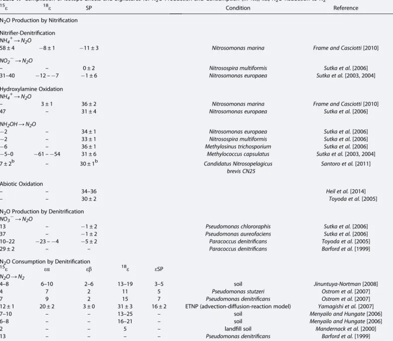
Table 1. Compilation of Isotope Effects and Signatures for N₂O Production and Consumption (in‰), i.e., N₂O Reduction to N₂^a

15ε ¹⁸ε SP Condition Reference

N₂O Production by Nitrification Nitrifier-Denitrification NH₄⁺→N₂O

58 ± 4 8 ± 1 11 ± 3 Nitrosomonas marina Frame and Casciotti[2010]

NO₂→N₂O

– – 0 ± 2 Nitrosospira multiformis Sutka et al. [2006]

31–40 12–7 1 ± 6 Nitrosomonas europaea Sutka et al.[2003, 2004]

Hydroxylamine Oxidation NH₄⁺→N₂O

– 3 ± 1 36 ± 2 Nitrosomonas marina Frame and Casciotti[2010]

47 – 31 ± 4 Nitrosomonas europaea Sutka et al.[2006]

NH₂OH→N₂O

2 – 34 ± 1 Nitrosomonas europaea Sutka et al.[2006]

2 – 33 ± 1 Nitrosospira multiformis Sutka et al.[2006]

6 – 36 ± 1 Methylosinus trichosporium Sutka et al.[2006]

5–0 61–54 31 ± 6 Methylococcus capsulatus Sutka et al.[2003, 2004]

7 ± 2^b – 30 ± 1^b Candidatus Nitrosopelagicus

brevis CN25

Santoro et al.[2011]

Abiotic Oxidation

– – 34–36 Heil et al.[2014]

– – 30 ± 2 Toyoda et al.[2005]

N₂O Production by Denitrification NO₃→N₂O

13 – 1 ± 2 Pseudomonas chlororaphis Sutka et al.[2006]

37 – 1 ± 2 Pseudomonas aureofaciens Sutka et al.[2006]

10–22 23–4 5 ± 2 Paracoccus denitrificans Toyoda et al.[2005]

29 ± 2 – – Paracoccus denitrificans Barford et al.[1999]

N₂O Consumption by Denitrification

15ε εα εβ ¹⁸ε εSP

N₂O→N₂

4–8 6–10 2–6 13–19 3–5 soil Jinuntuya-Nortman[2008]

4 7 2 11 5 Pseudomonas stutzeri Ostrom et al.[2007]

7 9 2 15 7 Pseudomonas denitrificans Ostrom et al.[2007]

12 ± 1 20 ± 2 3 ± 0 31 ± 3 16 ± 2 ETNP (advection-diffusion-reaction model) Yamagishi et al.[2007]

7–10 – – 13–25 – soil Menyailo and Hungate[2006]

6–8 – – 16–21 – soil Menyailo and Hungate[2006]

2 – – 5 – landfill soil Mandernack et al.[2000]

13 – – – – Pseudomonas denitrificans Barford et al.[1999]

aSee Figure 1 for complete reactions.

bThe exact mechanism, isotope effects and SP for N₂O production by Archaea are still not well constrained.

Nonzero SP arises from the differential biochemical bond making and breaking experienced by each of the two N atoms as a consequence of their different molecular positions (Figure 1). For example, in the consump- tion of N₂O by denitrification, the bond between the O atom and theαN atom is broken. It would then be expected that any isotopic fractionation occurring during this process would mostly influence theαposition

15N/¹⁴N ratio thereby increasing the SP of the residual population of N₂O molecules.

The bulk isotopic composition (δ¹⁵N andδ¹⁸O) of N₂O depends in part on the isotopic composition of its sub- strates (Figure 1). In the case of hydroxylamine oxidation, bulk N₂Oδ¹⁵N andδ¹⁸O are functions of theδ¹⁵N of the source NH₄⁺andδ¹⁸O of dissolved O₂, respectively. For nitrifier-denitrification and denitrification, N₂O δ¹⁵N andδ¹⁸O is dependent on theδ¹⁵N andδ¹⁸O of source NO₃and/or NO₂. A further consideration is that significant O exchange usually occurs between NO₂ and H₂O during N₂O production by nitrifier- denitrification or denitrification [Wrage et al., 2005;Kool et al., 2011;Snider et al., 2012], which would decouple theδ¹⁸O values of source and product.

Isotopic fractionation during nitrification and denitrification is the other major influence on theδ¹⁵N andδ¹⁸O of N₂O. Kinetic isotope fractionation occurs as a consequence of differences in reaction rate for the isotopo- logues of a molecule (e.g.,¹⁴N,¹⁵N and¹⁶O,¹⁸O for N₂O). Typically, the molecules containing the lighter isotopes react more quickly leaving the residual substrate enriched in heavier isotopes (e.g.,¹⁵N and¹⁸O).

The isotope effect (ε) is defined here by

ε¼ððk₁=k₂Þ-1Þ 1000 (3)

wherek₁andk₂are the reaction rates for the lighter and heavier isotopes, respectively.

N and O isotope effects for (¹⁵ε,¹⁸ε) during N₂O production and consumption vary substantially in laboratory culture as well as in the environment, likely as a result of sensitivity to growth conditions and reaction rates [Lewicka-Szczebak et al., 2015] and perhaps unconstrained variations in substrate isotopic composition (Table 1). Of course, such variability can complicate the interpretation offield data.

In contrast to bulk isotope values, N₂O SP is independent of the initial isotopic composition of the substrate [Toyoda et al., 2002;Schmidt et al., 2004]. Thus, SP is only process-dependent and can be used as a robust tracer to identify the source of N₂O. For instance, low SP isotopic signatures (11 to 0‰) are associated with N₂O production via NO₂ reduction by nitrifier-denitrification or denitrification. Much higher SP values are indicative of N₂O production by hydroxylamine oxidation (30–36‰) [Sutka et al., 2006; Frame and Casciotti, 2010]. However, SP does increase as a result of isotope fractionation during consumption by deni- trification as discussed above [Yamagishi et al., 2005, 2007;Ostrom et al., 2007].

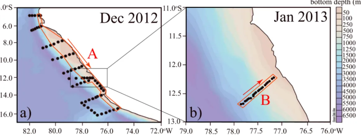
The main goal of this study is to identify the primary sources and sinks for N₂O in coastal waters of the ETSP using a natural stable isotope approach. In particular, we seek to understand the processes leading to near- surface, high N₂O concentrations that could contribute to highfluxes to the atmosphere. We present N₂O concentrations; isotope and isotopomer data for N₂O, NO₃, and NO₂, and other complementary physical and chemical parameters at two high-resolution coastal transects sampled off the coast of Peru in December 2012 (transect A) and January 2013 (transect B, Figure 2). We also used a 3-D-reaction-advec- tion-diffusion regional box model to diagnose physical mixing and biological N₂Ofluxes from thefield data and evaluate the contribution from different N₂O production processes in oxic and low-O₂waters and N₂O consumption versus production in the ODZ.

2. Materials and Methods

2.1. Sample Collection and Hydrographic Data

Samples were collected during two research cruises aboard the R/VMeteoron 2 to 23 December 2012 (M91) and 5 to 31 January 2013 (M92) (Figure 2), as part of the German projects SFB 754 (Climate-Biogeochemistry Interactions in the Tropical Ocean) and SOPRAN (Surface Ocean Processes in the Anthropocene). Water sam- ples were collected by using 12 L Niskin bottles (~23 depths per profile) on a conductivity-temperature-depth (CTD) rosette equipped with pressure, conductivity, temperature, and oxygen sensors. Oxygen and nutrient (NO₃, NO₂, NH₄⁺, and PO₄³) concentrations were measured on board as described in Stramma et al.[2013].

Samples for dissolved N₂O were collected in a similar fashion as for dissolved O₂/N₂/Ar samples [see Charoenpong et al., 2014]. Tygon tubing was attached to the Niskin bottle, and a 165 mL serum glass bottle wasfilled and overflowed with seawater at least 2 times before capping with a butyl stopper and crimp sealed with aluminum seal. This procedure was executed underwater in a plastic container to avoid air bub- bles. After collection, 0.2 mL of a saturated HgCl₂solution was injected to prevent biological activity.

Samples for N₂/Ar were collected similarly in 60 mL serum glass bottles and preserved with 100μL HgCl₂ [Charoenpong et al., 2014]. Duplicate N₂/Ar samples were collected at every other depth.

Samples for N and O isotopic composition of NO₃were collected in 125 mL plastic bottles and acidified for preservation (1 mL of 2.5 mM sulfamic acid in 25% HCl), which also served to remove NO₂at the time of sample collection [Granger and Sigman, 2009]. For NO₂ isotopic analysis, samples were collected and preserved with NaOH (2.25 mL of 6 M NaOH in 125 mL, pH = 12.5) to prevent oxygen isotope exchange with water during storage [Casciotti et al., 2007]. Samples were stored at room temperature before analysis.

2.2. N₂O Concentrations, Isotopes, and Isotopomers

Analyses were made by using a GV IsoPrime Continuous Flow, MultiCollector, Isotope-Ratio Mass Spectrometer (CF-MC-IRMS) coupled to an automated gas extraction similar to what is used for O₂/N₂/Ar samples [Charoenpong et al., 2014], with some modifications. Our IRMS has the necessary collector config- uration for simultaneous determination of masses 30, 31 for the NO⁺fragment of N₂O (determination of δ¹⁵N^α) and 44, 45, and 46 (determination ofδ¹⁵N^bulkandδ¹⁸O).

Briefly, seawater is pumped from sample bottles through a gas-extractor that is continuously sparged with He.

Dissolved N₂O was completely extracted into the He continuousflow and concentrated and purified in a purge- trap system. CO₂is chemically removed, and H₂O vapor is eliminated with both chemical and cryogenic traps.

N₂O is cryofocused with two liquid N₂traps and passed through a capillary gas chromatography (GC) column prior to IRMS analysis. These latter steps are nearly identical to those used byMcIlvin and Casciotti[2010] includ- ing GC column backflushing to eliminate interferences in the SP determination. For standardization, aliquots of gas standards are injected upstream of the gas-extractor to“experience”all extraction and purification steps.

We calibrated our measurements and corrected for scrambling between theαandβpositions [Westley et al., 2007] using N₂O standards covering a large range of SP (as well asδ¹⁵N^bulkandδ¹⁸O) composition (Table 2) [seeMohn et al., 2014]. These standards were analyzed in duplicate for each run to quantify the scrambling effect and potential offsets, and we iteratively solved for the different calibration parameters as described inFrame and Casciotti[2010] andMohn et al.[2014]. Correction for isobaric interference from¹⁷O is included in these procedures. We have optimized water and Heflows to achieve quantitative extraction and reprodu- cibility of results even at low N₂O concentration (down to ~5 nmol L¹). Instrumental drift was determined from measurements of the 5°C seawater standard distributed throughout an analytical run.

Standard deviations for triplicate measurements of our N₂O standards were typically below 0.1‰forδ¹⁵N^bulk- N₂O, 0.1‰forδ¹⁸O-N₂O, and 1.0‰for SP, which are comparable to values reported byMohn et al.[2014].

Figure 2.Maps showing stations sampled (black dots) during the (a) M91 cruise in December 2012 and (b) M92 cruise in January 2013. The two coastal transects (A and B, red rectangles) used for our analysis are shown.

N₂O concentrations in our sam- ples were calculated from relative peak heights between the sam- ples and a seawater standard of known N₂O concentration equili- brated with the atmosphere at 5°C (12.5 nmol L¹ at salinity 34 as calculated by using the Weiss and Price’s [1980] equation).

Equilibrium N₂O concentrations were calculated by using the global mean contemporary atmospheric N₂O dry mole fraction of 325 ppb in December 2012 and January 2013 (http://agage.mit.edu/data/

agage-data). We observed close agreement between the N₂O con- centrations measured with our IRMS and those measured indepen- dently byKock et al.[2016] by using gas chromatography and an elec- tron capture detector.

2.3. Biogenic N₂

N₂/Ar andδ¹⁵N-N₂measurements were made on septum-sealed samples by using an online gas extraction system coupled to a CF-MC-IRMS as described in Charoenpong et al. [2014]. Excess N₂ concentration ([N₂]_excess) inμmol L¹, the observed [N₂] minus the equilibrium [N₂] at in situ temperature and salinity, was calculated as inCharoenpong et al.[2014] and calibrated daily against seawater standards equilibrated with air atfixed temperature. Standard deviation for the samples was generally better than 0.7μmol L¹ for [N₂]_excess. We calculated biogenic [N₂] ([N₂]_biogenic), the [N₂] produced by denitrification or anammox, by subtracting the [N₂]_excessat a background station unaffected by N loss from the observed [N₂]_excessat corresponding potential density, as inBourbonnais et al.[2015]. This corrects for nonregional biological N loss as well as physically produced deviations in equilibrium N₂/Ar [Hamme and Emerson, 2002].

2.4. N and O Isotopic Composition of NO₃and NO₂

The stable isotopic compositions (δ¹⁵N andδ¹⁸O) of NO₃and NO₂were analyzed by using the“bacteria method”[Sigman et al., 2001;Casciotti et al., 2002] and the“azide method”[McIlvin and Altabet, 2005]. For NO₃isotopic analysis, samples were neutralized and NO₃was quantitatively converted to N₂O by cultured denitrifying bacteria that lack the active N₂O-reductase enzyme (Pseudomonas chlororaphis, ATCC #13985) [Casciotti et al., 2002]. Blank contribution was generally below 5% of the target sample size. For NO₂isotopic analysis, NO₂was converted to nitrous oxide (N₂O) by using sodium azide in acetic acid. The reagent was modified by increasing the acetic acid concentration to 7.84 M to account for high sample pH. N₂O gas was automatically extracted, purified, and analyzed online by using a purge-trap preparation system coupled to an IsoPrime CF-IRMS. Standard sample size was 20 nmol N₂O for NO₃isotope analysis and 15 nmol N₂O for NO₂isotope analysis. N and O isotope ratios are reported in per mil (‰), relative to AIR-N₂forδ¹⁵N and to VSMOW forδ¹⁸O as in equation (1).

NO₃ and NO₂ isotope data were calibrated by using the reference materials listed in Table 2 [see Casciotti and McIlvin, 2007]. The reproducibility was generally better than 0.2‰ for δ¹⁵N and 0.5‰ for δ¹⁸O in NO₃and NO₂.

2.5. Regional Box Model Description

We diagnosed the biologicalfluxes and ratios of N₂O production and consumption processes from the obser- vational data. We accounted for thefluidflowfield and physical mixing of N₂O and its isotopomers within

Table 2. N₂O, NO₃, and NO₂Standards Used for Sample Calibration (in‰)

δ¹⁵N^α δ¹⁵N^β δ¹⁸O δ¹⁵N^bulk SP N₂O

EMPA CB0897 15.7 3.21 35.2 6.245 18.91

EMPA CB0971 82.1 78 21.6 80.05 4.1

EMPA CB0976 5.55 12.9 32.7 3.675 18.45

EMPA 5350 1.71 94.4 36 48.055 92.69

NO₃

δ¹⁵N δ¹⁸O

IAEA N3 4.7 25.6

USGS 34 1.8 27.9

USGS 35 2.7 57.5

LABmix^a 38.9 –

NO₂

δ¹⁵N δ¹⁸O

MAA1^a 60.6 –

MAA2^a 3.9 –

Zh1^a 16.4 –

N23 3.7 11.4

N7272 79.6 4.5

N10219 2.8 88.5

aIn house standard.

regional box models spanning the spatiotemporal scales of our cruise collected data (see Figure S1 in the supporting information). The physical mixing was estimated by using physical circulation output from an eddy-resolving ROMS (Regional Ocean Modeling System [Shchepetkin and McWilliams, 2005]) simulation.

The ROMS model has been used to represent the regional mesoscale circulation in the Peru region with a model configuration similar to that inPenven et al.[2005]: it has a 1/9° × 1/9° spatial resolution (~12 km) and 32 vertical levels with a refined vertical resolution near the surface. For more details on the model con- figuration, the reader is referred toPenven et al.[2005]. This model has been validated against observations in previous works [e.g.,Echevin et al., 2011;Montes et al., 2011;Pietri et al., 2014]. Temperature and potential den- sity simulated from the ROMS and observed during both the M91 and M92 cruises agreed well (Figure S2). In the present study, it was forced by monthly open boundary conditions from the 1/4° GLORYS2V3 reanalysis over the period of 2007–2013 operated by Mercator-Ocean and downloaded on the Copernicus platform (http://marine.copernicus.eu). Advanced scatterometer daily wind stress processed by Centre ERS d’Archivage et de Traitement (http://cersat.ifremer.fr/), climatological heat and freshwater fluxes from Comprehensive Ocean-Atmosphere Data Set [Da Silva et al., 1994], and a restoring of sea surface temperature to advanced very high resolution radiometer optimum interpolation sea surface temperature daily data followingBarnier et al.[1995], were used at the ocean-atmosphere model interface.

A 70-box model was constructed to encompass the 56 stations sampled for N₂O and its isotopomers during the M91 cruise in December 2012. The 70-box model has dimensions 7 (lat) × 2 (lon) × 5 (depth), spanning 5–16°S, oriented at an angle of ~45° from north, which aligns the boxes with the Peru coastline (Figure S3). The longitudinal line separating the inshore (overlying the shelf) boxes from the offshore boxes follows the 300 m isobath. The top of depth level 1 (see Figure S3) begins below the surface mixed layer at 10 m depth as to ignore sea-air gas exchange of N₂O with the atmosphere.

A 25-box model was constructed to encompass the 13 stations sampled for N₂O and its isotopomers during the M92 cruise in January 2013. The 25-box model has dimensions 5 (lon) × 5 (depth, spanning 5–900 m) in the region covering 12.2 to 12.8°S and 77.0 to 77.9°W, oriented at an angle of ~ +45° from north, which aligns the boxes perpendicular with the Peru coastline (Figure S4).

Observed [N₂O],δ¹⁵N^α-N₂O, andδ¹⁵N^β-N₂O were interpolated onto the box model grid and averaged when multiple observations were included in a given model box. Physical mixing of N₂O and its isotopomers by horizontal advection, vertical advection (upwelling), and vertical diffusion between model boxes were con- sidered by using output from a regional ROMS simulation for the months of December 2012 and January 2013. Three-day averaged output of theu,v, andwvelocities (m/s) as well as the log-transformed vertical diffusivity coefficient (k_z; m²/s) were time averaged to obtain the monthly averaged circulation properties.

The 1/9° resolution ROMS output, which lies on a terrain-following (sigma) vertical grid, was interpolated onto the box model grid and averaged for a given model box. Advective velocities and vertical diffusivity were combined with [N₂O] and its isotopomer gradients to compute the physical mixing of tracers between model boxes as

∂½N₂Ophy

∂t ¼∇uN₂Oþ ∂

∂zwN₂Oþ ∂

∂zkz ∂

∂zN₂O (4)

∂δ¹⁵N^α½N₂O

phy

∂t ¼∇ uδ¹⁵N^αN₂O þ ∂

∂z wδ¹⁵N^αN₂O þ ∂

∂zkz ∂

∂z δ¹⁵N^αN₂O (5) with an equation analogous to equation (5) for mixing ofδ¹⁵N^β-N₂O. Horizontal diffusion of tracers was not considered, as the ROMS model is eddy-resolving and does not include an explicit diffusion scheme except near the model domain open boundaries [Penven et al., 2005]. The quantity∂[N₂O]_phy/∂twas substituted into equations (6)–(9) below to solve for the biological rates producing or consuming N₂O. Anoxic versus oxic boxes in the model were determined by interpolating cruise observed dissolved [O₂] onto the model grid by using a 5μmol L^-1[O₂] cutoff. Boundaryfluxes were computed by using ROMS velocities and vertical dif- fusivity output for the regions immediately to the north, south, and west of the box model domain as well as above (0–10 m depth) and below (300–350 m depth or bottom). N₂O tracer data for the boundaryfluxes were taken from the northernmost, southernmost, or westernmost stations as well as the mixed layer (0–10 m) and at depth (>300 m) where available.

The following equations describing the biologicalfluxes of N₂O and its isotopomers were used in shallow oxic waters ([O₂]>5μmol L^-1):

∂½N₂Obox

∂t ¼∂½N₂OND

∂t þ∂½N₂OHO

∂t þ∂½N₂Ophy

∂t (6)

SP_box∂½N₂Obox

∂t

¼ SP_ND∂½N₂OND

∂t

þ SP_HO∂½N₂OHO

∂t

þ ∂ðSP½N₂OÞphy

∂t

(7) where∂[N₂O]_box/∂tis the rate of N₂O concentration change for a given model box (sum of biological + mixing terms); SP_boxis the observed SP for a given box,∂[N₂O]_ND/∂t,∂[N₂O]_HO/∂t, SP_ND, and SP_HOare thefluxes and SPs from nitrifier-denitrification and hydroxylamine oxidation; and ∂(SP × [N₂O])_phy/∂t represents the physical mixing flux of SP × [N₂O] calculated as ∂(δ¹⁵N^α× N₂O)/∂t∂(δ¹⁵N^β× N₂O)/∂t (Table 1 and Figure S1).

The following equations were used for ODZ waters ([O₂]<5μmol L^-1):

∂½N₂Obox

∂t ¼∂½N₂OPD

∂t þ∂½N₂OCD

∂t þ∂½N₂Ophy

∂t (8)

SP_box∂½N₂Obox

∂t

¼ SP_PD∂½N₂OPD

∂t

ðSP_box εDÞ∂½N₂OCD

∂t

þ SP_phy∂½N₂Ophy

∂t

(9) where∂[N₂O]_PD/∂t and∂[N₂O]_CD/∂t are thefluxes from N₂O production and consumption by denitrification, εDis the isotope effect for SP during denitrification consumption, and SP_PDis the SP for denitrification production (Table 1 and Figure S1).

The box model assumes steady state, such that the sum of allfluxes into/out of (mixing) or within a box (bio- logical) equal zero.

3. Results

3.1. Distribution of O₂, Biogenic N₂, NO₃and NO₂Concentrations and Isotopes

Indicative of intense coastal upwelling, the mixed layer was always relatively shallow, i.e., ~5 m depth for transect A (Figure 3a), and less than 50 m depth at the deepest stations for transect B (Figure 4a). The oxycline ([O₂]<5μmol L¹), marking the upper ODZ boundary, became shallower from north to south along transect A varying from ~200 m at 6°S to ~20 to 50 m south of 10°S (Figures 3a and 4a). Along the outer shelf and slope, primary water masses were Antarctic Intermediate Water (AAIW; S≈34.5, T= 5.5°C) below 500 m and Equatorial Subsurface Water (ESSW; 34.7<S<34.9, 8.5°C<T<10.5°C) below the thermocline, with the latter corresponding to the low O₂ core of the southwardflowing Peru-Chile Undercurrent (PUC) [Strub et al., 1998]. Peru Coastal Waters (PCW; S≈35.0,T<19°C; referred to as Cold Coastal Waters inPietri et al.[2014]) were found next to the coast and mainly resulted from mixing between colder and slightly fresher upwelled waters from the PUC with Subtropical Surface Water (STSW;S>35, 20°C<T<28°C) [Strub et al., 1998] (Figure 5).

From north to south along transect A, subsurface waters reached the critically low levels of O₂required for the onset of N-loss processes (Figure 3). Biogenic N₂correspondingly increased as NO₃was consumed in the ODZ, with a maximum of ~20μmol L¹at 35 m depth at station 63 (Figure 3c). Relatively high biogenic N₂ concentrations were also observed in near-surface shelf waters south of 5°S, consistent with upwelling of ODZ waters impacted by N loss (Figures 3a, 3c and 4a, 4c).

This increase in biogenic N₂also corresponded to NO₂accumulations of up to 11μmol L¹in the coastal ODZ (50 m depth, station 64, transect A; Figure 3b). However, both NO₂and NO₃were almost completely consumed (<0.5μmol L¹) at the shallowest stations (station 63, transect A and station 9, transect B;

Figures 3b and 4b), which evidently had the highest extent of N loss.

Nitrateδ¹⁵N andδ¹⁸O increased with substrate consumption following isotopic fractionation during assimi- latory NO₃reduction by phytoplankton (ε= 5‰[Altabet, 2001]) and dissimilatory NO₃reduction in the coastal ODZ (ε= 15 to 25‰[Brandes et al., 1998;Voss et al., 2001;Granger et al., 2004, 2008;Bourbonnais

et al., 2015]) (Figures S5a and S5b). NO₂δ¹⁵N also generally increased with substrate consumption, as expected during NO₂reduction (ε= 8 to 22‰[Bryan et al., 1983;Brunner et al., 2013;Bourbonnais et al., 2015]) (Figures S5c and S5d).

3.2. N₂O Concentrations and Isotopomers

During transects A and B, supersaturating N₂O concentrations as high as 180 nmol L¹(station 26, transect A) occurred in oxygenated surface waters at a salinity of ~35 and temperature of ~15°C, characteristic of PCW [Pietri et al., 2014;Kock et al., 2016] (Figure 5) implying high potentialfluxes to the atmosphere. In contrast, ΔN₂O in the anoxic ODZ decreased from ~60 nmol L¹(station 10) to below saturating values (down to Figure 3.Key parameters for transect A along the Peru Coast (see Figure 2). (a) [O₂] withσθin overlay, (b) [NO₂] with [NO₃] in overlay, (c) biogenic N₂(from N₂/Ar data), (d)ΔN₂O, (e)δ¹⁵N^α-N₂O, (f)δ¹⁵N^β-N₂O, (g)δ¹⁸O-N₂O, and (h) SP. In Figure 3a, the depths of the different stations at a given latitude are indicated by red bars. Note that only one station was sampled for N₂O isotope and isotopomer analysis at a given latitude. CTD numbers are indicated at the top of Figure 3a. Bottom depth was ~300 m at the deepest station 10.

7 nmol L¹ at station 63) as a consequence of net consumption by denitrification. South of 5°S, the region of lowΔN₂O expanded vertically along with the ODZ and was correlated with N loss (transect A;

Figures 3c and 3d).

Some aspects of our observed coastal distribution of N₂O have also been found in offshore ODZ studies.

North of 5°N in the ETSP a N₂O maximum of ~60 nmol L¹was found in the oxygen minimum but further south a sharp double peak structure formed at the top and bottom of the ODZ with depletion within the core [Cohen and Gordon, 1978;Law and Owens, 1990;Kock et al., 2016]. However, the shapes for theΔN₂O in our near-coastal profiles were more variable and not as well defined as compared to offshore with significantly higherΔN₂O above the oxycline.

Figure 4.Key parameters for transect B normal to the Peru Coast (see Figure 2). (a) [O₂] withσθin overlay, (b) NO₂] with [NO₃] in overlay, (c) biogenic N₂(from N₂/Ar data), (d)ΔN₂O, (e)δ¹⁵N^α-N₂O, (f)δ¹⁵N^β-N₂O, (g)δ¹⁸O-N₂O, and (h) SP. CTD numbers are indicated at the top of Figure 4a. Bottom depth was ~2000 m at the deepest station 43.

N₂O isotopomer composition varied widely along both transects A and B. In oxygenated near-surface waters throughout the study region ([O₂]>5μmol L¹),δ¹⁵N^α-N₂O,δ¹⁵N^β-N₂O,δ¹⁸O-N₂O, and SP varied between 1 to 21‰,5 to 10‰, 40 to 79‰, and3 to 26‰, respectively (Figures 3, 4, and 6). The large range in δ¹⁸O-N₂O, in particular, was directly correlated with biogenic N₂ concentrations (transect A: r²= 0.49, p-value<0.05, n= 75; transect B: r²= 0.76, p-value<0.05, n= 22, at O₂>5μmol L^-1) and δ¹⁸O-NO₃ (Figures 7c and 7d). In the ODZ,δ¹⁵N^α-N₂O,δ¹⁸O-N₂O, and SP generally increased to up to 38‰, 93‰, and 56‰, respectively, as N loss increased with vertical expansion of the ODZ south of 5°S along transect A and toward the shelf (transect B). Interestingly,δ¹⁵N^β-N₂O generally remained the same or decreased as δ¹⁵N^α-N₂O and biogenic N₂increased in the coastal and offshore ODZs (Figures 3 and 4).

3.3. 3-D Reaction-Advection-Diffusion Box Modeling

The results from our regional box models showed high N₂O production rates of up to 49 nmol L¹d¹(trans- ect B, Figures 8a and 8e) in oxic waters. These rates were generally higher than those measured byJi et al.

[2015] from ¹⁵N-labeled incubations in offshore and coastal oxygenated waters in the ETSP (<1 nmol L¹d¹). N₂O production mainly occurred through nitrifier-denitrification (or incomplete denitrifier-denitrification as discussed below), which generally represented more than 50% of total N₂O pro- duction for transects A and B (Figures 8b and 8f and Tables S1 and S3 in the supporting information). N₂O production rates and the contribution from nitrifier (or incomplete denitrifier)-denitrification were also rela- tively high where the highest N₂O concentrations were observed (Figure 8).

In comparison,Frame et al.[2014] estimated that 64 to 68% of the N₂O production in the isotopic minimum of the upwelling zone off the southern African Coast was from nitrifier-denitrification using a simple model neglecting lateral and vertical advection/diffusion. Using a lower SP of11‰(as inFrame et al.[2014]) in our model decreased the contribution from nitrifier-denitrification (Tables S1 and S3). In addition, considering only vertical advection/diffusion generally decreased N₂O production rates with no clear effect on the parti- tioning between nitrifier-denitrification versus hydroxylamine oxidation (Tables S2 and S4). A major differ- ence between both study areas is that in contrast to the upwelling zone off the African Coast, the coastal waters off Peru overlay an ODZ, and therefore, in addition to nitrifier-denitrification, N₂O production is also likely to occur through incomplete denitrifier-denitrification.

N₂O production rates in the ODZ derived from our box model were up to 13.5 nmol L¹d¹when assuming an SP of0.5‰for N₂O production by denitrifier-denitrification [Sutka et al., 2006] and an isotope effect of either 5 or 16‰[Ostrom et al., 2007;Yamagishi et al., 2007] for SP during N₂O consumption by denitrification (Tables S1 and S3). Our N₂O production rates were in the same order of magnitude as those estimated from

15N-labeled incubations in the ETSP (up to ~4 nmol L¹d¹[Ji et al., 2015]) and from a 1-D model neglecting lateral advection in the ETNP ODZs (2 to 35 nmol L¹d¹[Babbin et al., 2015]). Measured N₂O consumption rates from tracer incubations byBabbin et al.[2015] in the ETNP ODZ balanced production and also agreed well with our modeled rates (up to ~40 nmol L¹d¹; Figures 8c and 8g).

N₂O consumption relative to production ranged from 12 to 96% for transect A and 0 to 100% for transect B (Figures 8d and 8h). Assuming a lower isotope effect of 5‰for SP during N₂O consumption Figure 5.Temperature-salinity plots for transects A and B (Figure 2) with color-codedΔN₂O (zaxis). The grey lines representσθ. Major water masses are indicated in bold (see section 3.1).

[Ostrom et al., 2007] increased relative N₂O consumption. The highest relative N₂O consumption in our model also usually occurred at the highest extent of N loss, where N₂O concentrations were below equilibrium, except at the shallowest station 9 (transect B) (Figures 3, 4, and 8).

4. Discussion

4.1. ExtremeΔN₂O in Upwelling Waters Resulting From Incomplete Denitrification

Throughout most of the ocean, subsurface waters isolated from the atmosphere slowly accumulate N₂O as a by-product of nitrification with progressive organic matter remineralization and O₂depletion. The subsurface intermediate waters entering the Peru coastal region in the form of the PUC have already experienced sub- stantial organic matter remineralization since their formation in the Subantarctic and thus enter our study region already low in O₂[Strub et al., 1998] and elevated in N₂O. Hence, nitrification during the course of water mass aging both outside as well as within the study region, via either the hydroxylamine oxidation or nitrifier-denitrification [Frame and Casciotti, 2010] pathway is a likely source for positiveΔN₂O concentra- tions (up to ~180 nmol L¹). This is particularly so for northern part of transect A which corresponds with the path of the southwardflowing PUC. N₂O further accumulates in this portion of transect A where N₂O produc- tion is active, but no N₂O consumption occurs, in the absence of denitrification. An exception to this Figure 6.(a and b) SP versusδ¹⁸O-N₂O, (c and d)δ¹⁵N^α-N₂O versusδ¹⁸O-N₂O and (e and f)δ¹⁵N^β-N₂O versusδ¹⁸O-N₂O for coastal transects A and B with color- coded [O₂] (zaxis). SP values for N₂O production by hydroxylamine oxidation, nitrifier-denitrification, and denitrification as well as for the modern troposphere (black stars [Yoshida and Toyoda, 2000]) are shown in Figures 6a and 6b. The pale grey dashed lines in Figures 6a–6d are the relationships between SP versusδ¹⁸O-N₂O andδ¹⁵N^αversusδ¹⁸O-N₂O expected during pure N₂O consumption by denitrification. The black lines are the linear regressions for samples with [O₂]<5μmol L¹. Stars next tor²values indicate significant relationships. The hexagons are data points from stations 63 (transect A) and 9 (transect B) showing an increase inδ¹⁵N^β- N₂O withδ¹⁸O-N₂O. Only shelf waters (<300 m depth for transect A and<500 m depth for transect B) were considered.

generality are instances of near-surface“hot spots”where incomplete denitrification may lead to some of the highest ΔN₂O values observed, as upwelled ODZ waters become modestly oxygenated inhibiting N₂O reduction to N₂ [Arévalo-Martínez et al., 2015; Kock et al., 2016]. N₂O may also accumulate disproportionately in our study region where O₂ is low given the possibility of increasing yield of N₂O production from nitrification under low oxygen concentrations [Goreau et al., 1980;Ji et al., 2015].

As N₂O-SP is only pathway-dependent [e.g.,Sutka et al., 2006], it can be used as a robust indicator of source pathway in the absence of consumption by denitrification. Production by nitrifier-denitrification (as well as denitrification) is associated with low SP values of11 to 0‰, whereas hydroxylamine oxidation produces higher N₂O-SP values of 30–36‰[Sutka et al., 2006;Frame and Casciotti, 2010] (Table 1). These laboratory results are mainly for bacterial ammonia oxidizers, whereas archaeal ammonia oxidizers, which are thought to be the dominant nitrifiers in the ocean [Santoro et al., 2011;Löscher et al., 2012], have been shown in cul- ture to produce N₂O with a high SP of 26–29‰, consistent with a hydroxylamine pathway. However, it was suggested that Archaea could also produce N₂O through NO₂reduction with lower SP in the environment [Santoro et al., 2011].

Figure 7.(a and b)δ¹⁵N-NO₃versusδ¹⁵N^bulk-N₂O, (c and d)δ¹⁸O-NO₃versusδ¹⁸O-N₂O, and (e and f)δ¹⁵N-NO₂versusδ¹⁵N^bulk-N₂O for transect A and B for [O₂]<5μmol L¹(blue circles and lines) and 50μmol L¹<[O₂]>5μmol L¹(red stars and lines). Only coastal waters (<500 m bottom depth) were considered. Stars next tor²values indicate significant relationships.

Throughout the nondentrifying portions of our study area (O₂>5μmol L^-1), relatively low SPs (3 to 26‰) were observed, with most values around ~3 to 14‰, especially for transect A (Figures 3, 4, and 6a, 6b). This and results from our box model (Figures 8b and 8f) suggest that nitrifier (or incomplete denitrifier)-denitrifi- cation is the dominant N₂O source.

Prior studies of Peru coastal waters note the occurrence of highΔN₂O in oxic ([O₂]>5μmol L¹) near-surface waters (up to 1000 nmol L¹[seeArévalo-Martínez et al., 2015;Kock et al., 2016]) (Figures 3d and 4d). In both transects A and B, highestΔN₂O (up to 180 nmol L¹) is found near surface at a number of stations (Figures 3 and 4). Though representing a minority of our samples, these patches of high N₂O are likely the most Figure 8.Results from the 3-D-reaction-advection-diffusion box models. Profiles of model (a and e) diagnosed rates of N₂O production in oxygenated waters ([O₂]>

5μmol L^-1) with N₂O concentrations in overlay, (b and f) diagnosed % N₂O produced from nitrifier-denitrification (ND) (or incomplete denitrifier-denitrification) relative to total N₂O production assuming a SP of 0‰for nitrifier-denitrification and 34‰for hydroxylamine oxidation, (c and g) diagnosed rates of N₂O consumption in the ODZ ([O₂]<5μmol L^-1) with N₂O concentrations in overlay, and (d and h) diagnosed % N₂O consumption by denitrification (CD) relative to consumption assuming a SP of0.5‰for N₂O production by denitrification and an isotope effect of 16‰during N₂O consumption along coastal transects A (Figures 8a–8d) and B (Figures 8e–8h). Individual data points represent the average value for each model box (see Figures S3 and S4). See Tables S1 to S3 for sen- sitivity of results to assuming different SP values and isotope effects.