www.biogeosciences.net/12/1537/2015/
doi:10.5194/bg-12-1537-2015
© Author(s) 2015. CC Attribution 3.0 License.
Organic carbon production, mineralisation and preservation on the Peruvian margin
A. W. Dale1, S. Sommer1, U. Lomnitz1, I. Montes2, T. Treude1,3, V. Liebetrau1, J. Gier1, C. Hensen1, M. Dengler1, K. Stolpovsky1, L. D. Bryant1, and K. Wallmann1
1GEOMAR Helmholtz Centre for Ocean Research Kiel, Kiel, Germany
2Instituto Geofísico del Perú (IGP), Lima, Peru
3Present address: University of California, Los Angeles (UCLA), USA Correspondence to: A. W. Dale (adale@geomar.de)
Received: 15 August 2014 – Published in Biogeosciences Discuss.: 9 September 2014 Revised: 18 January 2015 – Accepted: 6 February 2015 – Published: 11 March 2015
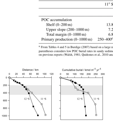
Abstract. Carbon cycling in Peruvian margin sediments (11 and 12◦S) was examined at 16 stations, from 74 m water depth on the middle shelf down to 1024 m, using a combina- tion of in situ flux measurements, sedimentary geochemistry and modelling. Bottom water oxygen was below detection limit down to ca. 400 m and increased to 53 µM at the deep- est station. Sediment accumulation rates decreased sharply seaward of the middle shelf and subsequently increased at the deep stations. The organic carbon burial efficiency (CBE) was unusually low on the middle shelf (<20 %) when com- pared to an existing global database, for reasons which may be linked to episodic ventilation of the bottom waters by oceanographic anomalies. Deposition of reworked, degraded material originating from sites higher up on the slope is pro- posed to explain unusually high sedimentation rates and CBE (>60 %) at the deep oxygenated sites. In line with other stud- ies, CBE was elevated under oxygen-deficient waters in the mid-water oxygen minimum zone. Organic carbon rain rates calculated from the benthic fluxes alluded to efficient min- eralisation of organic matter in the water column compared to other oxygen-deficient environments. The observations at the Peruvian margin suggest that a lack of oxygen does not greatly affect the degradation of organic matter in the water column but promotes the preservation of organic matter in sediments.
1 Introduction
The Peruvian upwelling forms part of the boundary current system of the Eastern Tropical South Pacific and is one of the most biologically productive regions in the world (Penning- ton et al., 2006). Respiration of organic matter in subsurface waters leads to the development of an extensive and peren- nial oxygen minimum zone (Walsh, 1981; Quiñones et al., 2010). Bottom water dissolved oxygen (O2) concentrations have been measured to be below the analytical detection limit from the shelf down to 400 m (Bohlen et al., 2011). Sedi- ments within this depth interval display organic carbon con- tents in excess of 15 % (Reimers and Suess, 1983a; Suess et al., 1987; Arthur et al., 1998); much higher than the average continental margin of<2 % (Seiter et al., 2004). Oxygen- deficient margins like Peru have thus been proposed to be sites of enhanced carbon preservation and petroleum-source rock formation (Demaison and Moore, 1980).
An understanding of the factors that enhance carbon preservation and burial in marine sediments is critical to in- terpret the sedimentary record and constrain global carbon sources and sinks over geological timescales (Berner, 2004;
Wallmann and Aloisi, 2012). Pioneering workers argued that carbon preservation is strongly driven either by the absence of O2in the bottom water (Demaison and Moore, 1980) or by higher primary production (Pedersen and Calvert, 1990).
Since then, much work on the biogeochemical characteristics of sediments has been undertaken to better disentangle these factors (Hedges and Keil, 1995; Arthur et al., 1998; Hedges et al., 1999; Keil and Cowie, 1999; Vanderwiele et al., 2009;
Zonneveld et al., 2010; and many others). These studies do broadly indicate that organic matter under oxic bottom wa- ters is in a more advanced state of degradation compared to oxygen-deficient waters. Investigations in the water col- umn have also shown that respiration of organic carbon is significantly reduced in oxygen-deficient waters, leading to elevated carbon fluxes to the sediments (Martin et al., 1987;
Devol and Hartnett, 2001; Van Mooy et al., 2002).
Rates of carbon burial and mineralisation on the Peru- vian margin have been studied as part of the Collaborative Research Center 754 (Sonderforschungsbereich, SFB 754, www.sfb754.de/en) “Climate-Biogeochemistry Interactions in the Tropical Ocean” (first phase 2008–2011 and second phase 2012–2015). The overall aim of the SFB 754 is to un- derstand the physical and biogeochemical processes that lead to the development and existence of oxygen-deficient regions in the tropical oceans. In this paper, in situ benthic fluxes and sedimentary geochemical data collected during two cam- paigns to the Peruvian margin at 11 and 12◦S are used to summarise our current understanding of carbon cycling in this setting. We address the following questions:
1. What is the rate of organic carbon mineralisation and burial in the sediments down through the oxygen mini- mum zone (OMZ)? Do these data point toward dimin- ished rates of organic carbon mineralisation in the water column?
2. Which factors determine the carbon burial efficiency at Peru and is there any marked difference for stations un- derlying oxic and anoxic bottom waters?
2 Study area
Equatorward winds engender upwelling of nutrient-rich equatorial subsurface water along the Peruvian coast (Fiedler and Talley, 2006). Upwelling is most intense between 5 and 15◦S where the shelf narrows (Quiñones et al., 2010). The sampling transects in this study at 11 and 12◦S are located within the same upwelling cell (Suess et al., 1987). The highest rates of primary productivity (1.8–3.6 g C m−2d−1) are 6 months out of phase with upwelling intensity due to the deepening of the mixed layer during the upwelling pe- riod (Walsh, 1981; Echevin et al., 2008; Quiñones et al.
2010). Austral winter and spring is the main upwelling pe- riod, with interannual variability imposed by the El Niño–
Southern Oscillation (ENSO) (Morales et al., 1999). The lower vertical limit of the OMZ is around 700 m water depth off Peru (O2<20 µmol kg−1; Fuenzalida et al. 2009). The mean depth of the upper boundary of the OMZ on the shelf at 11 and 12◦S is around 50 m (Gutiérrez et al., 2008), but deepens to ca. 200 m or more during ENSO years (e.g. Levin et al., 2002). At these times, dissolved O2 on the shelf can vary between 0 and 100 µM within a matter of days to weeks
as opposed to several months during weaker ENSO events (Gutiérrez et al., 2008; Noffke et al., 2012).
Sediments at 11 and 12◦S are generally diatomaceous, rapidly accumulating muds (Suess et al., 1987, and many others). Grain size analysis shows that clay/silt fractions are highest on the shelf and in mid-waters (>80 %), whereas the sand content is highest (40 %) in deeper waters (Mosch et al., 2012). The sediments can thus be described as sandy mud to slightly sandy mud (Flemming, 2000). The distribution of sediment on the margin is influenced by resuspension, win- nowing and lateral particle transport due to bottom currents and breaking of internal waves on the slope (Arthur et al., 1998; Levin et al., 2002; Mosch et al., 2012). Surface par- ticulate organic carbon (POC) content is high in mid-waters (15 to 20 %) with lower values (5 to 10 %) on the shelf and in deep waters (Böning et al., 2004).δ13C analysis and other geochemical indicators confirm that the organic matter at this latitude is almost entirely of marine origin (Arthur et al., 1998; Reimers and Suess, 1983b; Levin et al., 2002; Gutiér- rez et al., 2009).
The sediments down to around 400 m are notably cohe- sive, ranging from dark olive green to black in colour with no surface-oxidised layer (Bohlen et al., 2011; Mosch et al., 2012). The surface is colonised by dense, centimetre-thick mats of gelatinous sheaths containing microbial filaments of the large sulfur oxidising bacteria Thioploca spp. (Hen- richs and Farrington, 1984; Arntz et al., 1991). These bac- teria glide vertically through the sediments to access sul- fide, which they oxidise using nitrate stored within intracel- lular vacuoles (Jørgensen and Gallardo, 2006). The bacte- rial density varies with time on the shelf, depending on the bottom water redox conditions (Gutiérrez et al., 2008). Spi- onid polychaetes (ca. 2 cm length) have been observed in as- sociation with the mats (Mosch et al., 2012). The biomass of macrofauna generally tends to be highest in the OMZ but with low species richness, dominated by polychaetes and oligochaetes (Levin et al., 2002). At the lower bound- ary of the OMZ, high abundances of epibenthic megafauna such as ophiuroids as well as echinoderms, pennatulaceans, Porifera, crustaceans, gastropods and echinoderms have been observed (Levin et al., 2002; Mosch et al., 2012). Sedi- ments here are olive green throughout with a thin upper oxi- dised layer light green/yellow in colour (Bohlen et al., 2011;
Mosch et al., 2012).
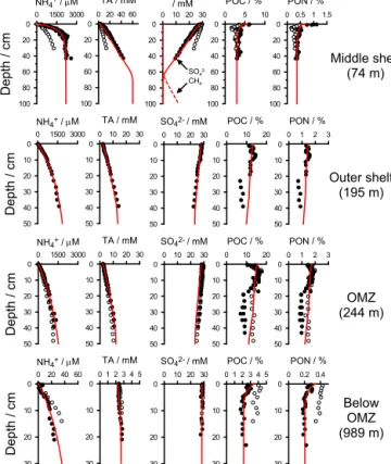
For the purposes of this study, we divide the Peruvian mar- gin into three zones broadly reflecting bottom water O2dis- tributions and sedimentary POC content: (i) the middle and outer shelf (<ca. 200 m, POC 5 to 10 %, O2<detection limit (dl, 5 µM) at time of sampling) where non-steady conditions are occasionally driven by periodic intrusion of oxygenated bottom waters; (ii) the OMZ (ca. 200 to 450 m, POC 10 to 20 %, O2predominantly<dl); and (iii) the deep stations be- low the OMZ with oxygenated bottom water (POC≤ca. 5 % and O2>dl).
−78.6 −78.5 −78.4 −78.3 −78.2 −78.1 −78 −77.9 −77.8 0
200 400 600 800 1000 1200
5
5 5
20 20
20
60
100 60 100
Depth [m]
Longitude
11°S Section
RV Meteor cruise M77/1 November 2008
O2 in µM
0 60 120 180 240
−77.7 −77.6 −77.5 −77.4 −77.3 −77.2 0
200 400 600 800 1000 1200
5 5
5 5 5
20 20
20
60
60 60
100
Depth [m]
Longitude
RV Meteor cruise M92/1 January 2013
0 60 120 180 240
< 5 µM
O2 in µM
12°S Section
< 5 µM
2 1 4 3 6 5
7 8
9
10
1
3 2 4
5
6
−100
−200
−200 -300
−500
−500
−1000
−1000
−2000
−3000
79°W 40’ 20’ 78°W 40’ 20’ 77°W 13°S
30’
12°S 30’
11°S 30’
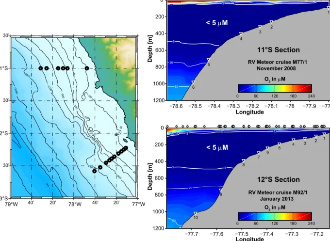
Figure 1. Slope bathymetry (contours in m) and benthic sampling stations on the Peruvian margin at 11 and 12◦S (left). The two panels on the right show cross-sections of dissolved oxygen concentrations (µM) measured using the CTD sensor calibrated against Winkler titrations (detection limit 5 µM). The station locations are indicated by the black triangles and the CTD stations used to make the plots are indicated by the grey diamonds.
3 Material and methods
3.1 Flux measurements and sediment sampling
We present data from six stations along 11◦S sampled during expedition M77 (cruise legs 1 and 2) in November/December 2008 and ten stations along 12◦S during expedition M92 (leg 3) in January 2013 (Fig. 1). Both campaigns took place dur- ing austral summer, i.e. the low upwelling season, and un- der neutral or negative ENSO conditions (http://www.cpc.
ncep.noaa.gov). With the exception of the particulate phases, the geochemical data and benthic modelling results from the 11◦S transect have been published previously (Bohlen et al., 2011; Scholz et al., 2011; Mosch et al., 2012; Noffke et al., 2012). Data from 12◦S are new to this study.
In situ fluxes were measured using data collected from Biogeochemical Observatories, BIGO (Sommer et al., 2008;
Dale et al., 2014). BIGO landers contained two circular flux chambers (internal diameter 28.8 cm, area 651.4 cm2). One lander at 11◦S, BIGO–T, contained only one benthic cham- ber. Each chamber was equipped with an optode to moni-
tor dissolved O2concentrations. A TV-guided launching sys- tem allowed smooth placement of the observatories on the seafloor. Two hours (11◦S) and 4 h (12◦S) after the lan- ders were placed on the seafloor, the chamber(s) were slowly driven into the sediment (∼30 cm h−1). During this initial period, the water inside the flux chamber was periodically replaced with ambient bottom water. After the chamber was driven into the sediment (∼10 cm), the chamber water was again replaced with ambient bottom water to flush out so- lutes that might have been released from the sediment during chamber insertion. The water volume enclosed by the ben- thic chamber ranged from 7.8 to 18.5 L and was mixed using a 5 cm stirrer bar at 140 rpm located 10–15 cm above the sed- iment surface. During the BIGO-T experiments, the cham- ber water was replaced with ambient bottom water halfway through the deployment period to restore outside conditions and then re-incubated.
Four (11◦S) or eight (12◦S) sequential water samples were removed periodically with glass syringes (volume of each syringe∼47 mL) to determine fluxes of solutes across
the sediment–water interface. For BIGO-T, four water sam- ples were taken before and after replacement of the chamber water. The syringes were connected to the chamber using 1 m long Vygon tubes with an internal volume of 6.9 mL. Prior to deployment, these tubes were filled with distilled water, and great care was taken to avoid enclosure of air bubbles. Con- centrations were corrected for dilution using measured chlo- ride concentrations in the syringes and bottom water. Water samples for gas measurements (12◦S) were taken at four reg- ular time intervals using 80 cm long glass tubes (internal vol- ume ca. 15 mL). An additional syringe water sampler (four or eight sequential samples) was used to extract ambient bot- tom water samples from 30–40 cm above the seafloor. The benthic incubations were conducted for time periods ranging from 17.8 to 33 h. Immediately after retrieval of the obser- vatories, the water samples were transferred to the onboard cool room set to the average bottom water temperature on the margin (8◦C) for further processing and sub-sampling.
Benthic fluxes were estimated from linear regressions of the concentration-time data and corrected for the volume to sur- face area ratio of the chamber. The volume was estimated on board using the mean height of water above the sediments in the recovered chambers.
Sediment samples for analysis were taken using multiple- corers (MUC) deployed adjacent to the BIGO sites. Re- trieved cores were immediately transferred to the cool room and processed within a few hours. Sub-sampling for redox sensitive constituents was performed under anoxic condi- tions using an argon-filled glove bag. Sediment samples for porosity analysis were transported to the on shore labora- tory in air-tight containers at 8◦C. Samples for porewater extraction were centrifuged at 4500 rpm for 20 min. Prior to analysis, the supernatant was filtered with cellulose acetate Nuclepore® filters (0.2 µm) inside the glove bag. The cen- trifugation tubes with the remaining solid phase of the sedi- ment were stored at−20◦C for further analysis on shore. Ad- ditional samples for bottom water analysis were taken from the water overlying the sediment cores.
3.2 Analytical details
Dissolved oxygen concentrations in the water column were measured using a Seabird SBE43 polarographic membrane oxygen sensor mounted on a SeaBird 911 CTD rosette sys- tem. The sensors were calibrated against discrete samples collected from the water column on each CTD cast and anal- ysed on board using Winkler titration with a detection limit of ca. 5 µM. The optodes inside the benthic chambers were calibrated by vigorously bubbling unfiltered bottom seawa- ter with air or argon for 20 min and calibrated using Win- kler. We broadly define O2concentrations below the detec- tion limit of the Winkler analysis as anoxic, whilst noting that sub-micromolar levels have been measured in the OMZ using microsensors (Kalvelage et al., 2013).
Ammonium (NH+4) was measured on board using stan- dard photometric techniques with a Hitachi U2800 photome- ter (Grasshoff et al., 1999). The detection limit was 1 µM and the precision of the analyses was 5 µM. Total alkalinity (TA) was determined by direct titration of 1 mL porewater with 0.02 M HCl using a mixture of methyl red and methylene blue as an indicator and bubbling the titration vessel with argon gas to strip CO2 and hydrogen sulfide. The analysis was calibrated using IAPSO seawater standard, with a pre- cision and detection limit of 0.05 meq L−1. Ion chromatog- raphy (Methrom 761) was used to determine sulfate (SO2−4 ) in the onshore laboratory with a detection limit of<100 µM and precision of 200 µM. Major cations were determined by ICP-AES with a detection limit and precision as given by Haffert et al. (2013).
The partial pressure of CO2 (pCO2) was analysed in the benthic chambers at 12◦S by passing the sample from the glass tubes (without air contact) through the membrane in- let of a quadrupole mass spectrometer (GAM200 IPI Instru- ments, Bremen). The samples were analysed sequentially, flushing with distilled water between samples. Standards of 300, 500, 1000 and 5000 ppm CO2were prepared by sparg- ing filtered seawater from the bottom water from each station using standard bottles of CO2of known concentration at in situ temperature for 30 min. Calibration was performed be- fore and after analysis of the samples from each site. The relative precision of the measurement was<3 %.
Wet sediment samples for analysis of POC and particu- late organic nitrogen (PON) were freeze-dried in the home laboratory and analysed using a Carlo-Erba element analyser (NA 1500). POC content was determined after acidifying the sample with HCl (0.25 N) to release the inorganic compo- nents as CO2. Weight percent of total carbon was determined using samples without acidification. Inorganic carbon was determined by weight difference between the total and or- ganic carbon. The precision and detection limit of the POC analysis was 0.04 and 0.05 dry weight percent (% C), respec- tively. The precision and detection limit of the inorganic car- bon analysis was 2 and 0.1 % C, respectively. Porosity was determined from the weight difference of the wet and freeze- dried sediment. Values were converted to porosity (water vol- ume fraction of total sediment) assuming a dry sediment den- sity of 2 g cm−3(Böning et al., 2004) and seawater density of 1.023 g cm−3. The analysis of total aluminium (Al) concen- trations in digestion solutions was carried out using an induc- tively coupled plasma optical emission spectrometer (ICP- OES, VARIAN 720-ES) following the procedure described by Scholz et al. (2011).
Additional samples from adjacent MUC liners taken from the same cast were used for the determination of down- core profiles of unsupported (excess) 210Pbxs activity by gamma counting. This approach includes the monitoring of the main peaks of anthropogenic deposition of241Am dur- ing the 1950s (test of nuclear weapons) as an independent time marker. Between 5 and 34 g of freeze-dried and ground
sediment, each averaging discrete 2 cm depth intervals, was embedded into a 2-phase epoxy resin (West System Inc.), all in the same counter-specific calibrated disc geometry (2 inch diameter). Following Mosch et al. (2012), a low-background coaxial Ge(Li) planar detector (LARI, University of Göttin- gen) was used to measure total210Pb via its gamma peak at 46.5 keV and226Ra via the granddaughter214Pb at 352 keV.
Prior to analysis,226Ra and214Pb in the gas-tight embedded sediment were allowed to equilibrate for at least 3 weeks. To determine210Pbxs, the measured total210Pb activity of each sample was corrected by subtracting its individual226Ra ac- tivity, assuming post-burial closed-system behaviour. Uncer- tainty of the210Pbxsdata was calculated from the individual measurements of 210Pb and226Ra activities using standard propagation rules. The relative error of the measurements (2σ) ranged between 8 and 58 %.
3.3 Calculation of dissolved inorganic carbon (DIC) fluxes
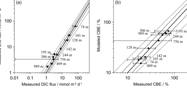
DIC concentrations in the benthic chambers at 12◦S were calculated from the concentrations of TA andpCO2using the equations and equilibrium coefficients given by Zeebe and Wolf-Gladrow (2001). Since four samples for pCO2 were taken using the glass tubes versus eight samples for TA anal- ysis in the syringes, each successive pair of TA data were averaged for calculating DIC (see Supplement). A constant salinity (35 psu), total boron concentration (0.418 mM) and seawater density (1.025 kg L−1) were assumed. For the shelf stations where sulfide was released from the sediment (Som- mer et al., unpub. data), corrections were made for the con- tribution of HS− to TA using the relevant equilibrium con- stants (Zeebe and Wolf-Gladrow, 2001). DIC fluxes were cal- culated from the concentrations as described above.
3.4 Determination of sediment accumulation rates Particle-bound210Pbxsis subject to mixing in the upper sed- iment layers by the movement of benthic fauna. The distri- bution of210Pbxscan thus be used to determine bioturbation coefficients as well as sedimentation rates using a reaction- transport model. We simulated the activity of 210Pbxs in Bq g−1 using a steady-state numerical model that includes terms for sediment burial, mixing (bioturbation), compaction and radioactive decay:
(1−ϕ(x))×ρ×∂210Pbxs(x)
∂t =
∂
(1−ϕ(x))×ρ×DB(x)×∂210Pbxs(x)
∂x
∂x
−∂ (1−ϕ(x))×ρ×vs(x)×210Pbxs(x)
∂x
+(1−ϕ(x))×ρ×λ210×Pbxs(x). (1)
In this equation,t (yr) is time, x (cm) is depth below the sediment–water interface, ϕ(x) (dimensionless) is poros- ity,vs(x) (cm yr−1) is the burial velocity for solids,DB(x) (cm2yr−1) is the bioturbation coefficient,λ(0.03114 yr−1) is the decay constant for210Pbxs andρ (2.0 g cm−3) is the bulk density of solid particles.
Porosity was described using an exponential function as- suming steady-state compaction:
ϕ(x)=ϕ (L)+(ϕ (0)−ϕ (L))×exp
− x zpor
, (2)
whereϕ(0)is the porosity at the sediment–water interface, ϕ(L)is the porosity of compacted sediments andzpor (cm) is the attenuation coefficient. These parameters were deter- mined from the measured data at each station (Table S2 in Supplement).
Sediment compaction was considered by allowing the sed- iment burial velocity to decrease with sediment depth:
vs(x)=ωacc×(1−ϕ(L))
1−ϕ(x) , (3)
whereωacccorresponds to the sediment accumulation rate of compacted sediments.
The decrease in bioturbation intensity with depth was de- scribed with a Gaussian-type function (Christensen, 1982):
DB(x)=DB(0)×exp(− x2
2×xs2), (4)
where DB(0) (cm2yr−1) is the bioturbation coefficient at the sediment–water interface andxs(cm) is the bioturbation halving depth.
The flux continuity at the sediment surface serves as the upper boundary condition:
F (0)=(1−ϕ(0))×ρ×
vs(0)×210Pbxs(0)−DB(0)× ∂210Pbxs(x)
∂x 0
, (5)
whereF (0) is the steady-state flux of 210Pbxs to the sedi- ment surface (Bq cm−2yr−1). The influx of210Pbxswas de- termined from the measured integrated activity of 210Pbxs multiplied byλ:
F (0)=λ×ρ
∞
Z
0
210Pbxs(x)×(1−ϕ (x))dx. (6)
210Pbxs was present down to the bottom of the core at the 74 m station (12◦S), implying rapid burial rates. Here,F (0) was adjusted until a fit to the data was obtained.
A zero gradient (Neumann) condition was imposed at the lower boundary at 50 cm (100 cm for the shallowest sta- tions at 12◦S). At this depth, all210Pbxs will have decayed
for the burial rates encountered on the Peruvian margin.
The model was initialised using low and constant values for
210Pbxsin the sediment column. Solutions were obtained us- ing the numerical solver NDSolve in MATHEMATICA 9 with a mass conservation>99 %.
The adjustable parameters (ωacc, DB(0), xs) were con- strained by fitting the210Pbxsdata. Unsupported210Pb mea- surements were not made at the 101 and 244 m station (12◦S) and sedimentation rates here were estimated from adjacent stations. Parameters and boundary conditions for simulat- ing210Pbxsat 12◦S are given in Table S2 and in Bohlen et al. (2011) for 11◦S. For some cores, the subsampling strat- egy revealed the detection of the anthropogenic enrichment peak of nuclide 241Am (co-analysed on 60 keV). This pro- vides an independent time marker in the profiles and poten- tial validation of the radiometric age model deduced from the
210Pbxs-based sediment accumulation rates.
3.5 Diagenetic modelling of POC degradation
A steady-state 1–D numerical reaction-transport model was used to simulate the degradation of POC in surface sediments at all stations. The model developed for 12◦S is based on that used to quantify benthic N fluxes at 11◦S by Bohlen et al. (2011) with modifications to account for benthic denitri- fication by foraminifera (Glock et al., 2013).
The basic model framework follows Eq. (1). Solutes were transported by molecular diffusion, sediment accumulation (burial) and non-local transport by burrowing organisms (bioirrigation) in oxygenated sediments below the OMZ.
Solid transport by burial and bioturbation was parameterised using the results of the210Pbxsmodel. Model sensitivity anal- ysis based on solute fluxes showed that bioirrigation rates were very low.
The model includes a comprehensive set of redox reac- tions that are ultimately driven by POC mineralisation. POC was degraded by aerobic respiration, denitrification, iron ox- ide reduction, sulfate reduction and methanogenesis. Man- ganese oxide reduction was not considered due to negligi- ble total manganese in the sediment (Scholz et al., 2011).
The rate of each carbon degradation pathway was determined using Michaelis–Menten kinetics based on traditional ap- proaches (e.g. Boudreau, 1996). DIC is produced by POC degradation only, that is, carbonate dissolution or precipita- tion are not included (see Results).
The total rate of POC degradation was constrained us- ing a nitrogen-centric approach based on the relative rates of transport and reactions that produce/consume NH+4. The procedure follows a set of guidelines that is outlined fully in Bohlen et al. (2011). The modelled POC mineralisation rates for 11◦S were constrained using both porewater con- centration data and in situ flux measurements of NO−3, NO−2 and NH+4. Dissolved O2 flux data were used as an addi- tional constraint at the deeper stations. The POC degradation rates at 12◦S were further constrained from the measured
DIC fluxes. The model output includes concentration pro- files, benthic fluxes and reaction rates, which are assumed to be in steady state. Note, however, that the bottom wa- ters on the middle shelf at 12◦S were temporarily depleted in NO−3 and NO−2 at the time of sampling. Although this leads to uncertainties in the rate of nitrate uptake by Thio- ploca, POC degradation rates remain well-constrained from the DIC fluxes.
The model was solved in the same way as described for
210Pbxs. The sediment depth ranged from 50 to 100 cm de- pending on the station (Boudreau, 1996). Measured solute concentrations and known or estimated particulate fluxes to the seafloor served as upper boundary conditions (Bohlen et al., 2011). At the lower boundary, a Neumann (zero flux) boundary was generally implemented. A steady-state solu- tion was obtained (invariant concentrations with time and sediment depth) with a mass conservation>99 %.
3.6 Pelagic modelling of primary production
Primary production was estimated using the high-resolution physical-biogeochemical model (ROMS-BioEBUS) in a configuration developed for the Eastern Tropical Pacific (Montes et al., 2014). It consists of the hydrodynamic model ROMS (Regional Ocean Model System; Shchepetkin and McWilliams, 2003) coupled with the BIOgeochemical model developed for the Eastern Boundary Upwelling Systems (BioEBUS, Gutknecht et al., 2013). BioEBUS de- scribes the pelagic distribution of O2and the N cycle under a range of redox conditions with twelve compartments: phyto- plankton and zooplankton split into small (flagellates and cil- iates, respectively) and large organisms (diatoms and cope- pods, respectively); detritus; NO−3; NO−2; NH+4; dissolved organic N; and a parameterisation to determine nitrous ox- ide (N2O) production (Suntharalingam et al., 2000, 2012).
The model configuration covers the region between 4◦N and 20◦S and from 90◦W to the west coast of South Amer- ica. The model horizontal resolution is 1/9◦ (ca. 12 km) and has 32 vertical levels that are elongated toward the sur- face to provide a better representation of shelf processes.
The model was forced by heat and freshwater fluxes derived from COADS ocean surface monthly climatology (Da Silva et al., 1994) and by the monthly wind stress climatology computed from QuikSCAT satellite scatterometer data (Liu et al., 1998). The three open boundary conditions (north- ern, western and southern) for the dynamic variables (tem- perature, salinity and velocity fields) were extracted from the Simple Ocean Data Assimilation (SODA) reanalysis (Carton and Giese, 2008). Initial and boundary conditions for bio- geochemical variables were extracted from the CSIRO Atlas of Regional Seas (CARS 2009; for NO−3 and O2) and Sea- WiFS (O’Reilly et al., 2000; for chlorophylla). Other bio- geochemical variables were computed following Gutknecht et al. (2013) and Montes et al. (2014). Monthly chlorophyll climatology from SeaWiFS was used to generate phytoplank-
0 0.5 1 210Pbxs /
Bq g-1
30 20 10 0
Depth / cm
St. 1 74 m
0 0.5 1 1.5 210Pbxs /
Bq g-1
St. 4 142 m
0 0.5 1 1.5 210Pbxs /
Bq g-1
St. 5 195 m
0 0.5 1 1.5 210Pbxs /
Bq g-1
St. 7 306 m
0 0.1 0.2 210Pbxs /
Bq g-1
St. 8 409 m
0 0.5 1 1.5 210Pbxs /
Bq g-1
St. 9 756 m
0 0.1 0.2 0.3 210Pbxs /
Bq g-1
St. 10 989 m
0 0.5 1 1.5 210Pbxs /
Bq g-1
St. 3 128 m
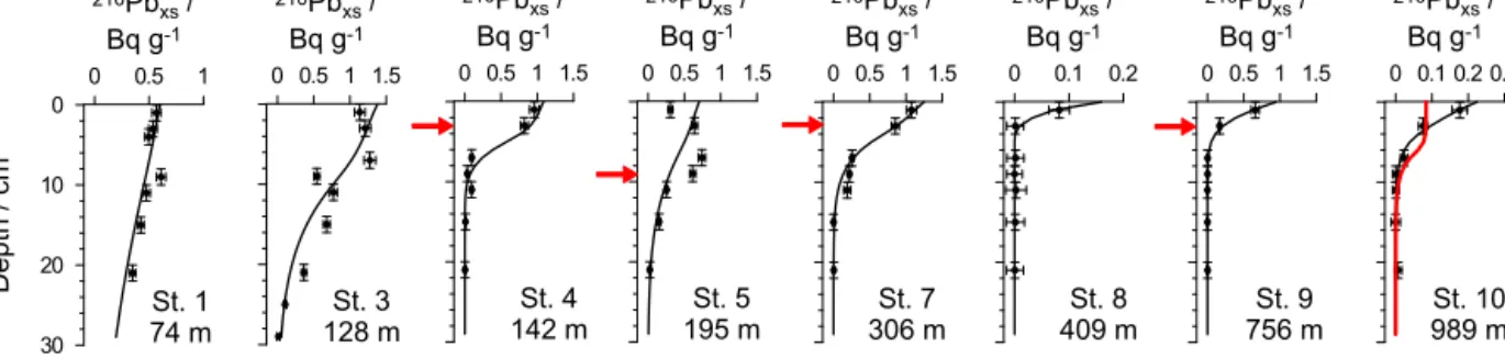
Figure 2. Measured (symbols) and modelled (curves)210Pbxsat 12◦S (see Bohlen et al. (2011) for210Pbxsat 11◦S). Vertical error bars span the depth interval from where the sample was taken, whereas horizontal error bars correspond to the analytical uncertainty. Derived upper boundary fluxes and bioturbation coefficients are listed in Table S2. The red arrows indicate the profile steps reflecting the detection of241Am and indicating the depth-position of the peak with activities as follows: St. 4=3.7±1.0 Bq kg−1; St. 5=5.8±0.99 Bq kg−1; St. 7=6.6±0.95 Bq kg−1; St. 9=2.2±0.68 Bq kg−1. The accuracy of the peak depth is defined by the sampling resolution. The red curve at St. 10 shows the results of a model simulation using the234Th-derived bioturbation coefficient of 100 cm2yr−1(see Appendix A).
ton concentrations, which were then extrapolated vertically from the surface values using the parameterisation of Morel and Berthon (1989). Based on Koné et al. (2005), a cross- shore profile following in situ observations was applied to zooplankton, with higher concentrations near the coast.
The simulation period was 18 years: the first 13 years con- sidered the hydrodynamics only, and then the biogeochemi- cal model was coupled for the following 5 years. The coupled model reached a statistical equilibrium after 4 years. The data presented here correspond to the final simulation year. De- tails of model configuration and validation are described by Montes et al. (2014).
Primary production (PP) was computed as the sum of the production supported by NO−3 and NO−2 uptake and regen- erated production of NH+4 uptake by nano- and microphy- toplankton (Gutknetch et al., 2013). Rates (in N units) were calculated for the station locations listed in Table 1 by in- tegrating over the euphotic zone. The atomic Redfield C : N ratio (106/16, Redfield et al., 1963) was used to convert PP into carbon units.
4 Results
4.1 Sediment appearance
Bottom sediments at 12◦S were very similar to those at 11◦S (see Sect. 2). The sediments down to ca. 300 m were cohe- sive, dark-olive anoxic mud (Gutiérrez et al., 2009; Bohlen et al., 2011; Mosch et al., 2012). Porosity was high on the shelf and in the OMZ (>0.9) deceasing to<0.8 at the deep- est stations (Fig. S1 in Supplement and Table 1). Porewa- ter had a strong sulfidic odour, especially in the deeper lay- ers. Shelf and OMZ sediments were colonised by mats of large filamentous bacteria, presumably Thioploca spp. (Gal- lardo, 1977; Henrichs and Farrington, 1984). Surface cover- age by bacterial mats was 100 % on the shelf and decreased to roughly 40 % by 300 m where the bacteria formed patches
0 200 400 600 800 1000 1200 Depth (m) 0
500 1000 1500 2000
MAR / g m-2 yr-1 (a)
0 200 400 600 800 1000 1200 Depth (m) 0
20 40 60
Al accumulation / g m-2 yr-1 (b)
Figure 3. (a) Bulk sediment mass accumulation rates and (b) alu- minium accumulation rates at 11◦S (open symbols) and 12◦S (closed symbols).
several decimetres in diameter. Mat density was much lower at 11◦S, not exceeding 10 % coverage (Mosch et al., 2012).
Thioploca trichomes extended 2 cm into the overlying water to access bottom water NO−3 (cf. Huettel et al., 1996) and were visible down to a depth of ca. 20 cm at the mat sta- tions. Polychaetes and oligochaetes were also present on the shelf, but not at the deeper stations within the OMZ. Despite anoxic bottom waters, no mats were visible at St. 8 (409 m, 12◦S). Sediments here consisted of hard grey clay under- lying a 2–3 cm porous surface layer that was interspersed with cm-sized phosphorite nodules. The upper layer con- tained large numbers of live foraminifera that were visible to the naked eye (J. Cardich et al., unpublished data). Sim- ilar foraminiferal “sands” containing phosphorite granules were noted at 11◦S, in particular below the OMZ (Mosch et al., 2012). Phosphorite sands on the Peruvian margin were found in areas of enhanced sediment reworking by bottom currents and the breaking of internal waves on the seafloor (Suess, 1981; Glenn and Arthur, 1988; Mosch et al., 2012). Below the OMZ, macrofauna were more preva- lent and included harpacticoids, amphipods, oligochaetes and large polychaetes.
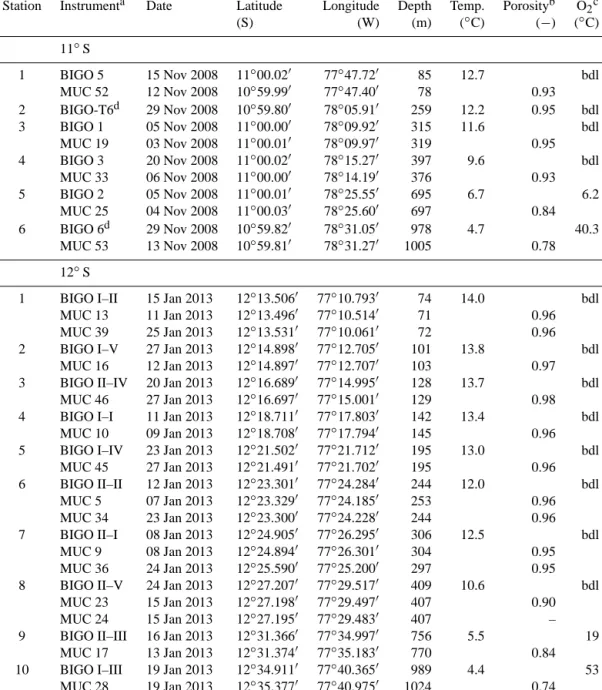
Table 1. Stations and instruments deployed on the Peruvian margin. Water depths were recorded from the ship’s winch. Bottom water temperature and dissolved oxygen are CTD measurements. Surface (0.5 cm, 11◦S; 0.25 cm, 12◦S) porosity values are also given.
Station Instrumenta Date Latitude Longitude Depth Temp. Porosityb O2c
(S) (W) (m) (◦C) (−) (◦C)
11◦S
1 BIGO 5 15 Nov 2008 11◦00.020 77◦47.720 85 12.7 bdl
MUC 52 12 Nov 2008 10◦59.990 77◦47.400 78 0.93
2 BIGO-T6d 29 Nov 2008 10◦59.800 78◦05.910 259 12.2 0.95 bdl
3 BIGO 1 05 Nov 2008 11◦00.000 78◦09.920 315 11.6 bdl
MUC 19 03 Nov 2008 11◦00.010 78◦09.970 319 0.95
4 BIGO 3 20 Nov 2008 11◦00.020 78◦15.270 397 9.6 bdl
MUC 33 06 Nov 2008 11◦00.000 78◦14.190 376 0.93
5 BIGO 2 05 Nov 2008 11◦00.010 78◦25.550 695 6.7 6.2
MUC 25 04 Nov 2008 11◦00.030 78◦25.600 697 0.84
6 BIGO 6d 29 Nov 2008 10◦59.820 78◦31.050 978 4.7 40.3
MUC 53 13 Nov 2008 10◦59.810 78◦31.270 1005 0.78
12◦S
1 BIGO I–II 15 Jan 2013 12◦13.5060 77◦10.7930 74 14.0 bdl
MUC 13 11 Jan 2013 12◦13.4960 77◦10.5140 71 0.96
MUC 39 25 Jan 2013 12◦13.5310 77◦10.0610 72 0.96
2 BIGO I–V 27 Jan 2013 12◦14.8980 77◦12.7050 101 13.8 bdl
MUC 16 12 Jan 2013 12◦14.8970 77◦12.7070 103 0.97
3 BIGO II–IV 20 Jan 2013 12◦16.6890 77◦14.9950 128 13.7 bdl
MUC 46 27 Jan 2013 12◦16.6970 77◦15.0010 129 0.98
4 BIGO I–I 11 Jan 2013 12◦18.7110 77◦17.8030 142 13.4 bdl
MUC 10 09 Jan 2013 12◦18.7080 77◦17.7940 145 0.96
5 BIGO I–IV 23 Jan 2013 12◦21.5020 77◦21.7120 195 13.0 bdl
MUC 45 27 Jan 2013 12◦21.4910 77◦21.7020 195 0.96
6 BIGO II–II 12 Jan 2013 12◦23.3010 77◦24.2840 244 12.0 bdl
MUC 5 07 Jan 2013 12◦23.3290 77◦24.1850 253 0.96
MUC 34 23 Jan 2013 12◦23.3000 77◦24.2280 244 0.96
7 BIGO II–I 08 Jan 2013 12◦24.9050 77◦26.2950 306 12.5 bdl
MUC 9 08 Jan 2013 12◦24.8940 77◦26.3010 304 0.95
MUC 36 24 Jan 2013 12◦25.5900 77◦25.2000 297 0.95
8 BIGO II–V 24 Jan 2013 12◦27.2070 77◦29.5170 409 10.6 bdl
MUC 23 15 Jan 2013 12◦27.1980 77◦29.4970 407 0.90
MUC 24 15 Jan 2013 12◦27.1950 77◦29.4830 407 –
9 BIGO II–III 16 Jan 2013 12◦31.3660 77◦34.9970 756 5.5 19
MUC 17 13 Jan 2013 12◦31.3740 77◦35.1830 770 0.84
10 BIGO I–III 19 Jan 2013 12◦34.9110 77◦40.3650 989 4.4 53
MUC 28 19 Jan 2013 12◦35.3770 77◦40.9750 1024 0.74
aThe first Roman numeral of the BIGO code for 12◦S denotes the lander used and the second to the deployment number of that lander. For 11◦S, the Arabic number refers to the deployment number. The lander at St. 2 is denoted BIGO-T (see text).bFull porosity profiles are given in the Supplement.cbdl=below detection limit (5 µM).dThese deployments occurred during leg 2 of cruise M77. All others from 11◦S took place during leg 1.
4.2 Sediment mixing and accumulation rates
At most stations, 210Pbxs distributions decreased quasi- exponentially and showed little evidence of intense, deep mixing by bioturbation (Fig. 2 and Bohlen et al., 2011); a feature that is supported by the lack of large bioturbating or- ganisms in and below the OMZ. The highest bioturbation co-
efficient determined by the model was 4 cm2yr−1for St. 3 at 12◦S (Table S2).
Mass accumulation rates (MAR) derived from 210Pbxs modelling (Fig. 3a) were similar to values reported previ- ously (Reimers and Suess, 1983c). Rates were extremely high at the shallowest stations (1200 and 1800 g m−2yr−1 at 11 and 12◦S, respectively). These are a factor of 2–3 times higher than measured elsewhere on the transects and
Table2.Measuredandmodelledcarbonfluxesandburialefficiencies. InnershelfOutershelfOMZBelowOMZ 12◦StransectSt.1St.2St.3St.4St.5St.6St.7St.8St.9St.10 Measureddata Waterdepth,m74101128142195244306409756989 Sedimentaccumulationrate(ωacc),cmyr−1a0.450.320.20.040.10.070.050.0110.0350.06 Massaccumulationrate(MAR),gm−2yr−1b180076860012832018215044259540 POCcontentat10cm(POC10),%c3.33.87.28.612.814.215.55.24.01.8 POCaccumulationrateat10cm(POCAR10),gCm−2yr−1d6029341141262321010 BenthicDICflux(JDIC),mmolm−2d−1e65.9±2127.9±4.220.4±78.0±0.43.2±14.7±12.7±0.12.2±0.32.8±31.2±0.1 POCrainrate(RRPOC),mmolm−2d−1f79.5±3334.2±1128.2±1210.5±312.5±610.6±48.0±22.7±15.2±53.4±1 Carbonburialefficiencyat10cm(CBE),%g17±719±628±1224±774±3755±2366±1919±646±4864±19 Modelleddata POCaccumulationrateat10cm,gCm−2yr−1h592934938272621112 BenthicDICflux,mmolm−2d−161.827.918.08.45.24.94.02.23.31.7 POCrainrate,mmolm−2d−1j75.334.525.910.613.911.110.02.65.84.4 Carbonburialefficiencyat10cm,%k18193020625660154361 PrimaryproductionfromROMS,mmolm−2d−11221151101071019692877773 11◦StransectSt.1St.2St.3St.4St.5St.6 Measureddata Waterdepth,m85259315397695978 Sedimentaccumulationrate(ωacc),cmyr−1m0.30.060.050.050.080.052 Massaccumulationrate(MAR),gm−2yr−1b1200132150370464343 POCcontentat10cm(POC10),%n2.414.215.312.66.83.8 POCaccumulationrateat10cm(POCAR10),gCm−2yr−1d291923463213 Modelleddata POCaccumulationrateat10cm,gCm−2yr−1h311617443216 BenthicDICflux,mmolm−2d−1p8.27.75.94.01.72.1 POCrainrate,mmolm−2d−1j15.311.49.814.09.05.9 Carbonburialefficiencyat10cm,%k473240718164 PrimaryproductionfromROMS,mmolm−2d−11129491888076 aDeterminedfrom210Pbxs(seeTableS2intheSupplement).SedimentationratesatSt.2(101m)andSt.6(250m)werenotmeasuredandinsteadestimatedfromtheneighbouringstations.ωacchasa20%uncertainty.bCalculatedasωacc×(1−ϕ(L))×ρ× 10000(ρ=drysoliddensity,2gcm−3).cForSt.8at12◦S(409m)thecontentat3cmwastakensincetheunderlyingsedimentisold,non-accumulatingclay.FortheOMZstationsthemeanPOCcontentintheupper10cmwasusedinstead.Thiswas approximatedasfollows:POC10(%)=1 10 10R 0POC(x)dxwherePOC(x)isin%.dCalculatedasMAR×POC10/100.eMeanfluxescalculatedfromtheinsituTAandpCO2measurementsintwobenthicchambers.NopCO2measurementsweremadeat 11◦S.Errorsrepresent50%ofthedifferenceofthetwofluxes.fCalculatedasPOCAR10(inmmolm−2d−1)+JDIC.gCalculatedasPOCAR10(inmmolm−2d−1)/RRPOC×100%.Errorswerecalculatedusingstandarderrorpropagationrulesassuming a20%uncertaintyinωaccandPOC10.hCalculatedanalogouslytofootnotedusingmodelleddata.jCalculatedanalogouslytofootnotefusingmodelleddata.kCalculatedanalogouslytofootnotegusingmodelleddata.mDeterminedfrom210Pbxsmodelling (seeBohlenetal.,2011).nFortheOMZstations,themeanPOCcontentintheupper10cmwasused(seefootnotec).pCalculatedasthedepth-integratedPOCdegradationrate(Bohlenetal.,2011).