Oxygen Variability and Tropical Atlantic Circulation
Cruise No. M130
August 28 – October 3, 2016 Mindelo (Cape Verde) – Recife (Brazil)
Marcus Dengler and Shipboard Scientific Party
GEOMAR Helmholtz-Zentrum für Ozeanforschung Kiel
Editorial Assistance:
DFG-Senatskommission für Ozeanographie
MARUM – Zentrum für Marine Umweltwissenschaften Bremen
2017
Table of Content
1 Cruise summary... 3
1.1 Summary in English ... 3
1.2 Zusammenfassung ... 3
2 Participants ... 4
3 Research program ... 5
4 Narrative of the cruise ... 6
5 Preliminary results... 8
5.1 Hydrographic observations ... 8
5.1.1 CTD system, oxygen measurements, and calibration ... 8
5.1.2. Oxygen Winkler measurements ... 9
5.1.3 Thermosalinograph... 9
5.2 Current observations ... 10
5.2.1 Vessel mounted ADCP... 10
5.2.2 Lowered ADCP ... 11
5.3 Mooring operations ... 11
5.3.1 Calibration of moored instruments ... 14
5.4 Shipboard microstructure measurements ... 15
5.5 Biochemical measurements ... 16
5.5.1 Tracermeasurements ... 16
5.5.2 Zooplankton ecology and particle dynamics ... 17
5.5.3 Nutrient sampling and analysis ... 18
5.5.4 N2 fixation, primary productivity ... 19
5.5.5 Iron biogeochemistry and utilization by marine diazotrophs ... 21
5.6 Aerosol concentrations ... 21
5.7 Expected results... 22
6 Weather report and meteorological station ... 23
7. Station list ... 25
7.1 General station list ... 25
7.2 CTD Station list ... 30
7.3 List of mooring deployments and recoveries ... 32
7.4 Biochemical sampling list ... 43
8 Data and sample storage and availability ... 44
9 Acknowledgements ... 44
10 References ... 44
11 Appendix – list of abbreviations (excerpt) ... 45
1 Cruise summary
1.1 Summary in English
A physical - biogeochemical survey was carried out in the northeastern tropical Atlantic and in the western tropical South Atlantic. The main objective of the works in the oxygen minimum zone of the eastern tropical North Atlantic was to improve oxygen budget estimates. Additional objectives were to investigate the role of zooplankton for fluxes of particulate and dissolved organic matter and to advance quantitative understanding of nitrogen fixation in the tropical Atlantic. The main objective of the measurements program in the western tropical South Atlantic was to investigate the variability of transport and water mass properties of the western boundary circulation.
A major component of the work program was the recovery of nine and the redeployment of eight moorings. The moorings positioned off Cape Verde, in the tropical northeastern Atlantic and at the western boundary off Brazil are collecting velocity, oxygen, temperature, and salinity time series since several years. All moorings were successfully recovered and redeployed. Section work focused on 23°W from 15°N to 5.5°S, on 11.5°S from 32°W to the coast of Brazil and on 5°S from 29.5°W to the coast of Brazil. Parameters measured along the sections included temperature- salinity-depth, oxygen and turbulence profiles, lowered acoustic Doppler current profiles, underwater vision profiles, shipboard velocity profiles, multinet and Working Party 2 net casts, and photosynthetically active radiation profiles. Water samples were analyzed for numerous variables including salinity, oxygen concentrations, tracer concentrations (CFC-12, SF6, CF3SF5), nutrients in micro and nano range, and halocarbons. Filtered samples were taken for NanoSIMS, flow cytometry, dissolved organic phosphorus, DNA/RNA, particulate organic matter, particulate organic nitrogen, and chlorophyll a. Samples of Heme content and dissolved iron were taken from a towed trace metal clean fish. Furthermore, on-board incubations to quantify nitrogen and carbon fixation and primary productivity were performed. The measurement program was successfully completed and all data sets were acquired as planned.
1.2 Zusammenfassung
Auf dem Fahrtabschnitt M130 wurde ein physikalisches-biogeochemisches Messprogramm in nordöstlichen und südwestlichen tropischen Atlantik durchgeführt. Die Hauptzielsetzung der Arbeiten in der Sauerstoffminimumzone des nordöstlichen tropischen Atlantiks war die Quantifizierung der Variabilität von Sauerstofftransportprozessen. Zusätzlich wurde der Einfluss von Zooplankton auf Flüsse von partikulärem und gelöstem organischen Material untersucht und die Nährstoffproduktion durch Stickstofffixierung bestimmt. Die Zielsetzung der Untersuchungen im westlichen tropischen Südatlantik war die Bestimmung der Variabilität der Randstromtransporte und der Wassermassen vor der Küste Brasiliens.
Eine Hauptkomponente der Arbeiten war die Bergung von 9 und erneute Auslegung von 8 Verankerungen. Die seit mehreren Jahren vor den Cape Verden, im tropischen Nordatlantik und vor der Küste Brasiliens existierenden Tiefseeverankerungen liefern Zeitserien von Strömungen, Sauerstoffgehalt, Temperatur und Salzgehalt. Alle Verankerungsarbeiten konnten erfolgreich abgeschlossen werden. Die Beprobung eines meridionalen Schnitts entlang 23°W (15°N bis 5.5°S) und zwei zonaler Schnitte entlang von 11°S (32°W bis Küste Brasiliens) und 5°S (29.5°W bis Küste Brasiliens) im westlichen Südatlantik wurde erfolgreich durchgeführt. Dabei wurden Temperatur-, Salzgehalts-, Druck-, Strömungs- und Turbulenzprofile aufgenommen,
Planktonproben mit Multinetzen und WP2 Netz gesammelt, photosynthetisch aktive Strahlungsprofile gemessen, Bilder mit einer Unterwasserkamera aufgezeichnet und Wasserproben genommen. Anhand der Wasserproben wurden die Konzentrationen von einer Vielzahl unterschiedlicher physikalischer und biogeochemischer Variablen bestimmt, darunter Sauerstoff, Salzgehalt, Tracer (CFC-12, SF6, CF3SF5), Nährstoffe in Mikro- und Nanobereich und Halogenkohlenwasserstoffe. Zusätzlich wurden Filtrate für NanoSIMS und Durchflusszytometrie erstellt und Proben für die Bestimmung von DNA/RNA, gelösten organischen Phosphat, partikulären organischen Kohlenstoff und Stickstoff sowie Chlorophyll a genommen. Proben für die Heme und Eisenbestimmung wurden mit einem spurenmetallfreien Gerät gesammelt.
Messungen zur Bestimmung der Rate der Stickstoffstofffixierung und der Primärproduktion wurden an Deck mit Inkubatoren durchgeführt.
2 Participants
No. Name Discipline Institution
1 Dengler, Marcus, Dr. Physical Oceanography / Chief scientist GEOMAR 2 Al Balushi, Hajar Physical Oceanography / LADCP GEOMAR 3 Bruto, Leonardo, Dr. Physical Oceanography / Moorings UFPE 4 Burmeister, Kristin Physical Oceanography / Mooring proc. GEOMAR 5 Caricchio Espinheira, Camilla Observer Brazilian Navy 6 Dürschlag, Julia Marine Biology / N2-fixation MPI Bremen 7 Faustmann, Jannik Marine Biology / Multinet, WP 2 net GEOMAR 8 Fernandez Carrera, Ana, Dr. Marine Biology / N2-fixation UVIGO 9 Gutekunst, Sören Dr. Marine Chemistry / Tracer, CFC-12, SF6 GEOMAR 10 Hahn, Johannes, Dr. Physical Oceanography / Optodes GEOMAR 11 Hauschildt, Jaard Physical Oceanography / Moored profiler GEOMAR 12 Hemmen, Joost Physical Oceanography / Aerosols GEOMAR 13 Ivanciu, Ioana Physical Oceanography / T, S, P - logger GEOMAR 14 Kiko, Rainer Dr. Marine Biology / UVP, multinet, driftnet GEOMAR
15 Kloewer, Milan Physical Oceanography /MSS GEOMAR
16 Krahmann, Gerd, Dr. Physical Oceanography / CTD and LADCP GEOMAR 17 Kriest, Iris, Dr. Marine Biology / Multinet, nutrients GEOMAR 18 Li, Pingyang Marine Chemistry / Tracer, CFC-12, SF6 GEOMAR 19 Link, Rudolf Physical Oceanography / CTD tech. GEOMAR 20 Louropoulou, Evangelia Marine Chemistry / Heme, nutrients GEOMAR 21 Maas, Josefine Marine Chemistry / Oxygen titration, CHBr3 GEOMAR 22 Niehus, Gerd Physical Oceanography / Moorings tech. GEOMAR 23 Papenburg, Uwe Physical Oceanography / Moorings tech. GEOMAR 24 Patey, Matt, Dr. Marine Chemistry / Nano-nutrients GEOMAR 25 Philippi, Miriam Marine Biology / N2-fixation, incubation MPI Bremen 26 Rohleder, Christian Meteorology / Bordwetterwarte DWD 27 Stöven, Tim, Dr. Marine Chemistry / Tracer, CFC-12, SF6 GEOMAR 28 Subramaniam, Ajit, Dr. Marine Biology / Biooptics, N2-fixation LDEO 29 Wagner, Partick Physical Oceanography / T, S, P – logger GEOMAR 30 Witt, Rene Physical Oceanography / Optodes tech. GEOMAR GEOMAR GEOMAR Helmholtz-Zentrum für Ozeanforschung Kiel
DWD Deutscher Wetterdienst, Geschäftsfeld Seeschiffahrt
LDEO Lamont Doherty Earth Observatory at Columbia University MPI Bremen Max-Planck Institute for Marine Microbiology
UVIGO Universidade de Vigo
UFPE Universidade Federal de Pernambuco
3 Research program
The research program was an integral component of the DFG Collaborative Research Center
”Climate - Biogeochemistry Interactions in the Tropical Ocean“ (SFB 754) and the BMBF- collaborative project “Regional Atlantic Circulation and Global Change” (RACE II). Within the framework of the SFB 754 the main scientific questions addressed during M130 were: (1) How does subsurface dissolved oxygen in the tropical ocean respond to variability in ocean circulation and ventilation? (2) What are the relations and feedbacks linking low or variable oxygen levels and key nutrient source/sink mechanisms in the water column? The cruise contributed to the research objectives by quantifying variability of ventilation processes of the oxygen minimum zone (OMZ) of the eastern tropical North Atlantic (ETNA) including oxygen fluxes due to lateral mixing, vertical mixing and lateral advective fluxes. A particular objective related to research question (2) was to quantify oxygen consumption within the OMZ. This was approached by tracer concentration measurements to assess the age of the tracers and hence water masses in the OMZ and by investigating the role of zooplankton and its vertical migration for fluxes of particulate and dissolved matter. Additionally, quantitative understanding of nitrogen fixation in the tropical Atlantic was advanced by measuring nitrogen fixation rates.
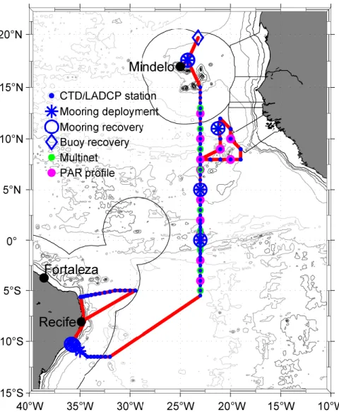
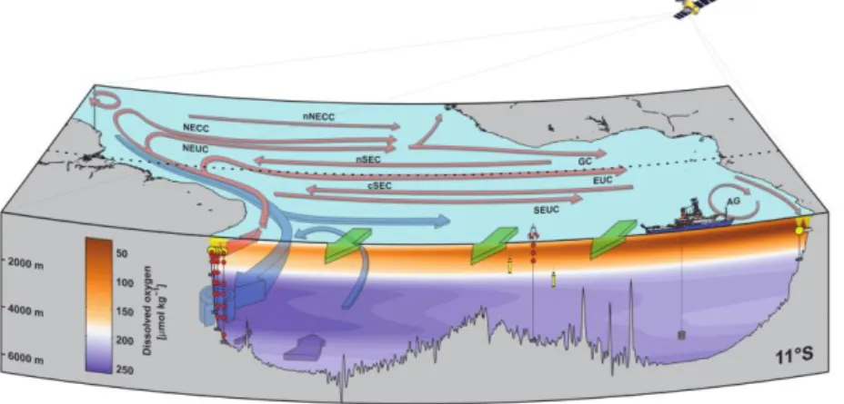
Fig. 3.1. Bathymetric map with cruise track of R/V METEOR cruise M130 (red solid line) including locations of CTD/LADCP stations, mooring recoveries and redeployments, multinet and photosynthetically active radiation (PAR) profile stations. Territorial waters of different countries are marked with thin black solid lines.
Within the framework of RACE II, the aim of this cruise is to investigate the variability of the western boundary current system off Brazil as well as providing a contribution for an estimate of the Atlantic meridional overturning circulation (AMOC) at 11°S. A particular focus at the western boundary will be on the transport variability of the North Brazil Undercurrent (NBUC) – as part of the AMOC and the subtropical cells (STCs) – on timescales from intraseasonal to decadal.
4 Narrative of the cruise
Due to a late arrival of a one of our container carrying dangerous goods in Mindelo, São Vicente, Cape Verde, the departure of R/V METEOR was delayed by one day. Customs cleared the delayed container in the morning of August 29 and we were able to leave port at 11:00 local time (12:00 UTC). The working program started 6 hours later with a successful recovery of a mooring at the Cape Verde ocean observatory (CVOO) site 50 nautical miles (nm) northwest of São Vicente. During the night, a full-depth profile with the conductivity-temperature-depth-oxygen (CTD/O2) rosette system was measured and plankton samples with a multinet were collected. The main CVOO mooring was successfully recovered in the early morning of August 30. After additional CTD, multinet and microstructure stations and trace metal clean water sampling using a towed fish, R/V METEOR left the CVOO site for an emergency recovery of a drifting buoy about 150 nm to the northeast. The buoy was originally deployed off Cape Blanc just outside the EEZ of Mauritania and had broken loose a month before our cruise. It weight 2.3 tons, had a diameter of 3 m and was equipped with a dust collector for investigating Saharan dust deposition.
Additionally, meteorological sensors were attached to the buoy. The rescue of the buoy, owned by the Royal Netherlands Institute of Sea Research (NIOZ), was coordinated jointly with the DFG Senatskommission für Ozeanographie, the Leitstelle Deutsche Forschungsschiffe and the National Marine Faculty at NIOZ. Prior to the recovery, it was agreed that NIOZ would refund the dedicated ship time within the OFEG barter ship-time framework. Thanks to the professionalism of R/V METEOR’s crew, the recovery of the buoy was completed within a few hours, minimizing the loss of ship time for our cruise. The vessel returned to the CVOO site on Sep. 1 at 4:00 UTC to redeploy the CVOO mooring and to collect additional water samples with the CTD rosette system and the towed fish. The CVOO related activities were completed 13h later at 17:00 UTC.
CTD/O2 section work along 23°W started at 15°N on September 2, 10:00 UTC and ended at 5.5°S on September 19, 10:30 UTC. CTD/O2 profiles were collected from the surface to a depth of 1200m between 15°N and 5.5°N and to full ocean depth between 5°N and 5.5°S. In addition to the CTD/O2 sensors and the attached underwater vision system, a chlorophyll sensor, turbidity sensor and an optical nitrate sensor was attached to the rosette frame. The latter could only be used during CTD casts to a depth above 2000 m. In addition, an upward and a down-looking acoustic Doppler current profiler (LADCP) were attached to the rosette frame to measure full depth velocity profiles. Apart from CTD profiles, spectroradiometer profiles were collected every mid-day to infer the distribution of photosynthetically active radiation in the upper 100 m of the water column, multinet casts were performed to a depth of 1000m at several positions along the transect for the sampling of zooplankton and microstructure profiles of velocity shear and temperature were collected to infer mixing levels required for determining diapycnal oxygen and nutrient fluxes.
Water sampling focused on resolving the vertical spreading of an artificial tracer (CF3SF5) that was released in the center of the oxygen minimum zone at 11°N, 21°S in December 2012 and on biogeochemical parameters including nutrients and chlorophyll to advance understanding of
nitrogen fixation. Additionally, two shipboard ADCPs with a frequency of 38 kHz and 75 kHz were continuously sampling horizontal velocities in the upper 600 and 1000 m, respectively, and two thermosalinographs were measuring near-surface temperature and salinity. All systems worked well throughout the cruise. However, in the morning of September 11 contact to the tethered microstructure profiler was lost while the profiler was descending during a microstructure (MSS) station at 6°S, 23°W. When we attempted to recover the profiler using its own winch, the microstructure cable broke and the profiler (serial number 32) was lost. The most likely explanation for the broken cable is that it was damaged by the bite of a fish. Microstructure measurements performed later during the cruise were done with a spare profiler (serial number 26) that had an identical sensor setup.
In the afternoon of September 5, the 23°W transect was discontinued to conducted a survey focussing on determining the variability of the artificial tracer concentrations in the region between 8°N and 11.5°N, 19°W and 23°W. Water samples were taken at stations where tracer concentrations had been determined during the previous R/V METEOR cruises M97, M105 and M116. During the survey, a mooring at 11°N, 21°13’W was recovered and redeployed in the morning and evening of September 8, respectively. This position approximately marks the center of the oxygen minimum zone of the tropical Atlantic. The mooring was equipped with velocity, temperature, salinity and oxygen sensors. The tracer survey was completed in the morning of September 10.
In the morning of September 11, a mooring at 23°W, 5°N was recovered. The mooring’s instrumentation was identical to those deployed at the 11°N mooring. Similar to the 11°N mooring, all sensors had worked well, but some of the oxygen loggers had stopped data recording early - a few weeks or months after mooring deployment in 2015. This error was due to a falsely adjusted operational mode of the recording units that caused elevated power consumption. R/V METEOR
reached the equator just after midnight on September 15. In the morning of that day, the equatorial mooring was successfully recovered and redeployed in the afternoon. Again, all sensors had worked well and we were particularly happy to have retrieved complete velocity, temperature, oxygen and salinity time series from a moored profiler that climbed the mooring wire between 1000m and 2500m depth.
After finalizing the 23°W section in the morning of September 19, R/V METEOR headed southwest towards the western boundary off Brazil. During the two-day transit a crossing-the-line ceremony and the “Bergfest” provided a welcomed change. The work program along the 11°S section started at 11.5°S, 32°W in the evening of September 21. During the 11°S section work, four moorings were recovered and redeployed and the data of two pressure-inverted echo sounders were read-out using acoustic modems. All mooring operations went well and we were very happy about the returned data - 37 of the 38 instruments mounted to the moorings recorded full data sets.
Additionally, 20 full-depth CTD/O2 profiles were collected along the 11°S section. The last CTD/O2 station along 11°S was completed shortly after midnight of September 27. The final CTD/O2 section along 5°S was started in the morning of September 28 and completed in the late afternoon of October 1. A total of 19 full depth CTD/O2 stations were collected at 5°S. R/V METEOR arrived as scheduled in the old port of Recife at 6:00 in the morning of October 3.
5 Preliminary results
In the following, a detailed account of the types of observations, methods and instruments used as well as some of the early results are presented.
5.1 Hydrographic observations
5.1.1 CTD system, oxygen measurements, and calibration (Gerd Krahmann, Jaard Hauschildt)
During M130, 118 profiles of pressure (P), temperature (T), conductivity (C) and oxygen (O) were recorded. While 69 of these CTD-O2 profiles ranged to the bottom or near the bottom, the remaining profiles ranged to 1200 m or shallower depth. We used a Seabird Electronics (SBE) 9plus system, attached to the water sampler carousel, and recent Seabird Seasave software (V7.23.2). The SBE underwater unit had, in addition to its own pressure sensor, two parallel sensor sets for T, C, and O. Additionally, a Wetlabs turbidity/chl a fluorescence sensor and a Wetlabs transmissometer was used on all casts (see table in section 7.2). Three altimeter systems were used during the cruise with different success. One system, manufactured by Teledyne Benthos, was able to reliably detect the sea floor during the CTDs approach. This system, however, transmits on a frequency that interferes with the lowered ADCPs, usually resulting in unreliable velocity profiles.
Two other systems, manufactured by Valeport, use a different frequency but were not able to detect the seafloor in waters greater than 3000m. We were not able to identify the reason for this malfunction (possibly a bad firmware version). As one of the major goals of the cruise was the collection of deep velocity profiles, we lowered the CTD without a sea floor warning to the depths of previous CTDs on the same position. Despite our cautious approach that typically stopped 30 to 100 m above the sea floor, the CTD touched ground during profile 59. A wire bent close to the CTD resulting from the grounding required the removal of some 30 m of wire and a new termination.
The CTD system itself performed without major problems and the same set of sensors was used throughout the whole cruise. As underwater unit was GEOMAR's SBE1 (SN #75760). Serial numbers of primary and secondary conductivity sensors were SN #2452 and SN #3373, respectively. Primary and secondary oxygen sensors were SN #0631 and SN #2592. Finally, serial numbers of temperature sensors were SN #4831 and SN #4823.
The usual procedures for calibration of the conductivity and oxygen sensors were performed.
Conductivity was calibrated using a linear relation in P, T and C and, in case of the secondary conductivity sensor, a temporal trend correction was additionally used. More than 400 water samples were collected for the conductivity calibration and analyzed using a GEOMAR's Guidline Autosal salinometers 8 and 4. Intermittent problems with the stability of the salinometers measurements lead to a switch from Autosal 4 to Autosal 8, which however showed similar instabilities of the measurement results. Nevertheless, the results are deemed accurate enough for the calibration of conductivity sensors to typical accuracies. The conductivity calibration resulted in a root mean square (rms) salinity misfit between 0.002 and 0.003 for the two sensors after removal of the most deviating 33% of samples. Oxygen was calibrated using a relation linear in T and O, and quadratic in P. Winkler titration of more than 1100 bottle samples led to a relation with an rms misfit of 0.9 µmol/kg (33% of bottle values removed).
Further sensors were attached to the carousel and recorded data, but were not calibrated: a fluorescence and turbidity sensor (FLNTU manufactured by Wetlabs), and an optical nitrate sensor
(SUNA manufactured by Satlantic). The latter could only be used during casts less than 2000 m deep.
5.1.2. Oxygen Winkler measurements (Josefine Maas)
Observing and understanding the concentration of dissolved oxygen in the ocean is one of the key objectives of the SFB754. While the CTD system is capable of measuring dissolved oxygen in the ocean at high vertical resolution, the sensors need to be carefully calibrated. Thus, very precise reference measurements are essential. During the entire cruise, water samples were taken for the determination of dissolved oxygen after Winkler (1888). Sampling was done with 100 ml WOCE bottles with well-defined volumes (calibrated flasks) to calibrate the oxygen sensors (SBE 43) and to support chemical and biological CTD data.
Oxygen samples were taken from the Niskin bottles immediately after tracer sampling. From each CTD/O2 cast, seven to eight water samples were taken. During the selection of sampling depth, regions of elevated vertical oxygen gradients identified from the CTD/O2 profile were avoided. Additionally, dissolved oxygen samples were taken from all bottles every second CTD station concurrently with tracer samples (see Section 5.5.1). For the entire cruise, this yields 1250 samples from 90 CTD casts.
The precision of the oxygen concentration measurements determined from Winkler titration was 0.37 μmol/L. This estimate is based on the arithmetical average of standard deviations from 15 duplicates and 68 triplicates.
The reagents used during the cruise were: sulfuric acid (50%), zinc iodide starch solution (500 mL, Merck KGaA), stock solution, fixation solution and standard solution. The stock solution consisted of sodium thiosulfate pentahydrate (49.5 g L-1). It was diluted by a factor of 10 to create the working solution (0.02 mol L-1). The fixation solution consisted of manganese (II) chloride (600 g L-1), sodium iodide (600 g L-1) and sodium hydroxide (320 g L-1). Potassium hydrogen diiodate (0,325 g L-1, homemade) was used for standard solution.
Standard measurements for the determination of the thiosulfate factor of the working solution were carried out on a daily basis. In addition to that, standard measurements were performed every time new reagents were applied. Titrations were performed within the WOCE bottles using a 20 mL Piston Burette (No. M 006989) TITRONIC universal from Schott Instruments. Dosing accuracy reported by the company is 0.15%, referred to the nominal volume, indicated as a measurement uncertainty with a confidence level of 95%. The iodate standard was added with a 50 mL Piston Burette (No. M 003550) TITRONIC universal from Schott Instruments. 1 mL of the fixation solutions (NaI/NaOH and MnCl2, respectively) were dispensed with a high precision bottle-top dispenser (0.4-2.0 mL, Ceramus classic, Hirschmann). Please note that possible errors from sampling, storing (air bubbles) or errors introduced while measuring were noted. Results derived from those measurements were not considered in the data precision estimate.
5.1.3 Thermosalinograph (Gerd Krahmann)
Two thermosalinograph systems are installed on R/V METEOR. Both systems are operated in parallel, system 1 drawing water from the port side, system 2 from starboard side of the ship. The comparison of the thermosalinograph temperatures with CTD temperatures from 5 m depth showed a very good agreement with no significant offset (-0.002 and -0.001°C for systems 1 and
2). The thermosalinograph’s salinities did however not agree as well with the CTD’s. For system 1, we found a difference of about -0.04 PSU (thermosal salinity minus CTD salinity) at the beginning of the cruise, which remained stable for about 10 days and then reduced in an approximately linear trend down to about -0.003 PSU. After day 23, however the salinity of system 1 changed the linear drift direction and reached nearly -0.02 PSU on day 33. System 2 also showed a significant drift but kept a constant direction and strength of the drift from -0.08 PSU at the beginning of the cruise to -0.04 PSU on day 33. Similar drifts and changes of drift direction have been seen on previous legs. As long as comparison samples from the well-calibrated CTD/water sampling system are frequently available, the deviations of thermosalinograph salinity appear to be correctable. The underlying cause for the drifts and in particular the changes in drift remains unclear, however.
Daily water samples were also taken from the thermosalinograph system and measured with GEOMAR's salinometers. Unfortunately, these data from the samples were available only on the last day of the cruise so that no time remained for a detailed comparison with the thermosalinograph calibration described above. Results from recent cruises have however shown good agreements between both approaches.
5.2 Current observations 5.2.1 Vessel mounted ADCP
(Kristin Burmeister, Camilla Caricchio Espinheira)
Underway current measurements of the upper ocean were performed continuously throughout the entire cruise track using two VMADCPs: a 75kHz RDI Ocean Surveyor (OS75) mounted in the ship’s hull, and a 38kHz RDI Ocean Surveyor (OS38) placed in the moon pool. Both Ocean Surveyor instruments worked well throughout the cruise. The OS38 was aligned to zero degrees (relative to the ship's centerline) in order to reduce interference with the OS75, which was aligned to 45 degrees.
The OS75 instrument was configured with 100 bins of 8 m, pinging 37.5 times per minute, with an averaged data range of 600 m. It was run in the more precise but less robust broadband mode until September 24. Due to a decrease in the range, the mode was switch to the more robust narrowband mode then. The OS38 instrument ran in narrowband mode and used 55 bins of 32 m, pinging 20 times per minute that resulted in a depth range between 1000 m and 1500 m. During the entire cruise, the SEAPATH navigation data was of high quality. To avoid interference with other acoustic devices, bathymetry measurements were performed using the 12kHz echo sounder EM122.
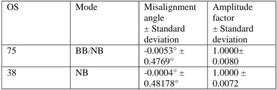
Table 5.1: Misalignment angle and amplitude factor of the Ocean Surveyors determined from water track calibration.
OS Mode Misalignment
angle
± Standard deviation
Amplitude factor
± Standard deviation
75 BB/NB -0.0053° ±
0.4769°
1.0000±
0.0080
38 NB -0.0004° ±
0.48178°
1.0000 ± 0.0072
Post processing of the data was carried out separately for each instrument. Accounting for a time shift of the heading and position data recorded by the SEAPATH device relative to the raw OS data allowed for a significant reduction in the scatter of the calibration angles and amplitude factors. The applied shifts, as well as mean misalignment angles and amplitude factors with the associated standard deviations, are summarized in Table 5.1.
5.2.2 Lowered ADCP (Gerd Krahmann)
During most of the cruise, the CTD/Rosette system was equipped with a lowered ADCP setup based on two Teledyne RDI ADCPs. The setup consisted of an up-looking and a down-looking 300 kHz instrument. These two instruments were mounted inside the CTD rosette with especially manufactured frames protecting the instruments and allowing zero obstruction of the acoustic beams. A battery pack was mounted below the up-looking slave. Both ADCPs were connected to the battery case, which was also the connection point for the data interface cable.
During the first 10 days of the cruise, several independent problems interfered with the collection of reliable LADCP data. During the initial installation one of the ADCP systems, SN
#20507 stopped communication with the control computer. During profile 6 the long communication cable between the battery container and the control computer in the GEO-lab malfunctioned, likely a broken internal communication chip. Subsequently we discovered two leaks in battery-container-to-ADCP cables, which prevented the slave system from operating properly. Lastly, a newly developed energy supply system that draws energy for the ADCPs from the CTD cable lead to malfunctions of the slave system and likely spurious error indications for the slave systems. Because of these error indications, four different ADCPs were used as slave until we realized the underlying energy supply problem. The master system remained the same throughout the whole cruise (SN #20508). As slave system, we used SN #11436 for profiles 1 to 7, SN #6468 for profiles 11 to 25, and SN 839 for profiles 26 and 27. As the broken system SN
#20507 was expected to perform best, we attempted to repair it by combining three internal boards from SN #11436 with the transducer head of SN #20507. This indeed worked and the hybrid SN
#20507/#11436 ADCP was used from profile 40 to 118.
During the cruise we used and further developed a simple to use software with which the start, stop, download, and erase cycles of the two LADCP systems can be controlled.
Data processing took place during the cruise using the GEOMAR LADCP processing software V10.21, which includes both shear and inversion methods to derive an absolute velocity profile.
As additional data are necessary for the processing, the corresponding pre-processed CTD files containing pressure, temperature and salinity profiles as well as time and navigation data were used.
Overall, the Teledyne RDI instruments resulted in reasonable to good deep ocean velocity profiles when processed in conjunction with the observations of the vessel-mounted ADCP (VMADCP) and when coming close enough to the seafloor to obtain TRDI bottom track data.
Nevertheless, the generally adverse conditions for LADCP in the open tropical South Atlantic Ocean (too few scatterers) lead to a several profiles with high uncertainties in particular along the 11°S transect.
5.3 Mooring operations
(Johannes Hahn, Kristin Burmeister, Patrick Wagner, Marcus Dengler)
Altogether, nine mooring were recovered, eight moorings were deployed and data from two pressure-inverted echo sounders (PIES) were collected using acoustic modems during the cruise (Table 5.2). With the exception of the oxygen sensors, the instruments recovered from the mooring had functioned very well. Table 5.3 shows the instrument performance for each mooring and sensor type calculated as the percentage of maximum obtainable data. For the calculation of the instrument performance, every instrument was weighted homogeneously taking the following instrument types into account: Mini-TD (T, P), MicroCAT (T, C, P), O2-Logger and Hydroflash O2 Optode (T, O2), ADCP (U, V), RCM (P, U, V), Argonaut (U, V), Aquadopp (P, U, V), moored profiler M-CTD MMP (T, C, U, V, O2), PIES (P), other (other parameters).
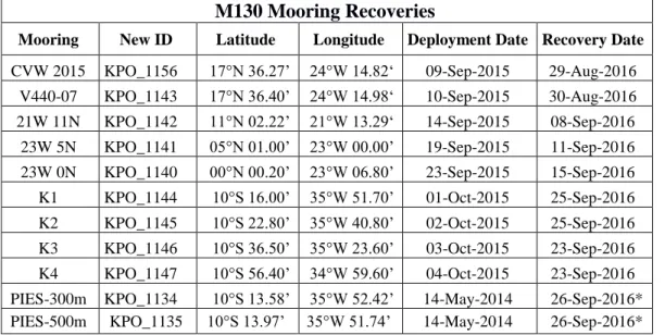
Table 5.2: Summary of mooring operations performed during the cruise.
M130 Mooring Recoveries
Mooring New ID Latitude Longitude Deployment Date Recovery Date
CVW 2015 KPO_1156 17°N 36.27’ 24°W 14.82‘ 09-Sep-2015 29-Aug-2016 V440-07 KPO_1143 17°N 36.40’ 24°W 14.98‘ 10-Sep-2015 30-Aug-2016 21W 11N KPO_1142 11°N 02.22’ 21°W 13.29‘ 14-Sep-2015 08-Sep-2016
23W 5N KPO_1141 05°N 01.00’ 23°W 00.00’ 19-Sep-2015 11-Sep-2016 23W 0N KPO_1140 00°N 00.20’ 23°W 06.80’ 23-Sep-2015 15-Sep-2016 K1 KPO_1144 10°S 16.00’ 35°W 51.70’ 01-Oct-2015 25-Sep-2016 K2 KPO_1145 10°S 22.80’ 35°W 40.80’ 02-Oct-2015 25-Sep-2016 K3 KPO_1146 10°S 36.50’ 35°W 23.60’ 03-Oct-2015 23-Sep-2016 K4 KPO_1147 10°S 56.40’ 34°W 59.60’ 04-Oct-2015 23-Sep-2016 PIES-300m KPO_1134 10°S 13.58’ 35°W 52.42’ 14-May-2014 26-Sep-2016*
PIES-500m KPO_1135 10°S 13.97’ 35°W 51.74’ 14-May-2014 26-Sep-2016*
* No recovery, acoustic communication and data download only.
M130 Mooring Deployments
Mooring New ID Latitude Longitude Deployment Date Recovery Date
V440-08 KPO_1179 17° 36.39’N 24° 14.98’W 01-Sep-2016 21W 11N KPO_1178 11° 02.22’N 21° 13.28’W 08-Sep-2016 23W 5N KPO_1177 05° 01.01’N 23° 00.00’W 11-Sep-2016 23W 0N KPO_1176 00° 00.06’S 23° 06.78’W 15-Sep-2016 K4 KPO_1172 10° 56.41’S 34° 59.60’W 24-Sep-2016 K3 KPO_1171 10° 36.50’S 35° 23.56’W 25-Sep-2016 K2 KPO_1170 10° 22.79’S 35° 40.78’W 26-Sep-2016 K1 KPO_1169 10° 15.99’S 35° 51.68’W 26-Sep-2016
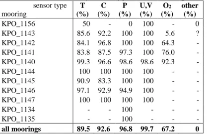
Instrument performance of better than 90% was reached for temperature, conductivity and pressure sensors as well as current meters. Oxygen sensors (O2-logger) performed only partly well (67%). The major problem of these sensors was the logger unit, which consumed too much battery due to a wrong setup of the board system. A summarized description over the performance of all instrument types is given in the following. Details of the moorings are shown in the mooring tables in section 7.3 below.
Out of the five temperature-depth recorders (Mini-TDs), three instruments had a complete and clean data record. One instrument (s/n 71) had a drift of the pressure sensor by 1-2 dbar throughout
the last three months of the mooring period. Communication to one instrument (s/n 64) was not possible after recovery (no data).
Table 5.3: Instrument performance in percent of data return by sensor type and mooring (T - temperature; C - conductivity; P - pressure; U,V - zonal, meridional velocity; O2 - oxygen; other – other parameters).
sensor type mooring
T (%)
C (%)
P (%)
U,V (%)
O2
(%) other
(%)
KPO_1156 50 - 0 100 - 0
KPO_1143 85.6 92.2 100 100 5.6 ? KPO_1142 84.1 96.8 100 100 64.3 - KPO_1141 83.8 87.5 97.3 100 76.0 - KPO_1140 99.3 96.6 98.6 98.6 92.3 -
KPO_1144 100 100 100 100 - -
KPO_1145 90.9 83.3 100 100 - -
KPO_1146 97.1 92.9 94.9 100 - -
KPO_1147 100 100 100 100 - -
KPO_1134 - - 100 - - -
KPO_1135 - - 100 - - -
all moorings 89.5 92.6 96.8 99.7 67.2 0
Recovered MicroCATs performed well and 38 out of 49 instruments provided a complete and clean record. One MicroCAT deployed close to the surface in KPO_1143 showed a bad conductivity cell for 3 days throughout the deployment period. Three MicroCATs (2933, 10609, and 2933) from KPO_1142 showed a bad conductivity cell for 16 days, one day and 4 months respectively. The same holds for one MicroCAT (2717) from KPO_1140, which had a bad conductivity cell for 5 days. The pressure sensors of two MicroCATs (10642, 6860) recovered at KPO_1143 and KPO_1141 showed a small drift of about 2dbar, while temperature and conductivity sensors worked fine. Two MicroCATs (2256, 2257), recovered at KPO_1143 and KPO_1141, respectively, had a corrupt memory status and provided no data at all. One MicroCAT (1286) was recovered damaged from KPO_1145 and provided no data due to water ingress. One MicroCAT (10712) recovered at KPO_1146 provided only 8 months of data for unknown reasons.
For collecting oxygen concentration time series, 20 optodes manufactured by AADI Aanderaa Data Instruments (subsequently named: O2-Logger) as well as two optodes from manufacturer Kongsberg Maritime Contros (subsequently named: Hydroflash O2 Optode) were installed in the recovered moorings. Only eight of the 20 O2-Logger performed with a complete and clean data record. The major problem of nine other O2-Logger was a too high battery consumption due to a wrong setup mode of the logger board yielding data records between 2 weeks and 7 months only.
The optode (s/n 147) of one logger had water ingress throughout the mooring period (only 3 months of data). One logger (s/n 1465) performed almost completely with a data coverage of 96%
(15 days of data are missing within six different intervals). The foil of the sensor of one optode (s/n 1461) was partly detached from the sensor throughout the mooring period and the data quality of this instrument needs to be carefully checked. Two optodes (s/n 219 and 942), aforementioned with a complete and clean data record, showed small marks of the sensor foil at one edge of the sensor spot. The sensor foils of the latter three optodes were changed after the onboard calibration.
The status of the two Hydroflash O2 Optodes remains unknown so far. However, the sensor foils of these two optodes had become completely detached from the sensors during recovery. It remains
unclear, whether this happened throughout the mooring period or during the instrument cleaning process after recovery.
All 21 single point current meter instruments (16 Aquadopps, 3 Argonauts, 2 RCM-11) performed well and provided complete and clean records. Furthermore, nine out of 10 ADCPs performed well and provided a complete and clean record. The QM14911 ADCP from KPO_1140 provided a complete record, but had problems with pitch and role. It was not redeployed but instead send to the manufacturer for maintenance after the cruise.
A McLane moored profiler (equipped with a CTD, a single point ADCP as well as an optode oxygen sensor) deployed in mooring KPO_1140 performed almost completely. It operated in the measurement range between 3500m and 1000m, where only during a few profiles the upper stopper at the mooring cable was not reached (due to ballasting issues or obstructions on the cable) or sensor measurements were partly bad, providing a data coverage of 89%.
Other instruments, such as two sediment traps in KPO_1143 had full bottles (no. 1-13). A fluorometer and a SAMI (CO2 sensor) performed completely, but the quality of the data is so far unknown. The winch with profiler in KPO_1156 had been already recovered one day after deployment during R/V METEOR cruise M119 (see this cruise report).
MicroCATs and O2-logger generally sampled using an interval of minimum 30 minutes and one hour, respectively. However, for O2 loggers and MicroCAT instruments deployed in the OMZ regime (KPO_1140, KPO_1141, KPO_1142), a sampling interval of 5 minutes was used to record variability from internal waves. For single point current meters and ADCPs, a sampling interval of one or two hours was used. The McLane moored profiler operated (upcast and subsequent downcast profile) every 4 days.
Mooring dynamics:
In general, moorings deployed in the western boundary current regime off Brazil as well as the mooring KPO_1143 located north of the Cape Verde Islands showed much higher dynamic variability than the moorings deployed in the moderate to sluggish flow regime of the eastern tropical North Atlantic (ETNA). The near-surface elements in the moorings off Brazil exhibited depth variability of 50 to 100 m with a maximum dive event of about 300 m (KPO_1147) on time scales of days to weeks. KPO_1143 had two dive events of 100 m and 150 m depth change for several weeks and two months, respectively. In contrast, depth variability of the ETNA moorings (KPO_1140, KPO_1141, KPO_1142) was very much reduced. Only few short dive events with about 100 m depth change occurred for mooring KPO_1141.
5.3.1 Calibration of moored instruments
CTD-O2 cast calibrations were performed for all Mini-TDs, MicroCATs and O2-Loggers either as pre- or post-deployment calibrations (CTD casts 001, 003, 005, 006, 020, 031, 035, 038, 041, 056, 058 067, 082, 088, 094, 109 and 113) by attaching the instruments to the CTD frame. Some additional O2-Loggers that were deployed on subsequent cruises were calibrated as well.
Aquadopps were attached to the CTD frame as well during casts 020, 067, 088 and 109 in order to test the performance of the temperature sensor.
During each upcast, 7-8 calibration stops were done over the whole profile range (depths chosen at low gradient-regimes for the respective parameters). In order to ensure equilibrium at the calibration stops, CTD heaving was discontinued for at least 4 minutes for Mini-TDs and MicroCATs calibration stops and 2.5 min for optode calibration stops. For MicroCATs, calibration
stops at around thermocline depth (upper few hundred meters of the water column) were prolonged by 1 minute. However, in test cases we found that even 5 to 10 minute-long calibration stops were too short (and had to be discarded afterwards) to achieve equilibrium within the conductivity cells of the MicroCATs. The long equilibration times are likely a result of the thermal mass effect. As an alternative, we partly conducted calibration stops of 5 minutes at 10 m depth before starting the regular downcast profile right at the beginning of the CTD cast. This approach reduced the average equilibration time of the MicroCat conductivity sensors.
Additionally, onboard lab calibrations were conducted for all O2-loggers in water-filled beakers of 0% and 100% O2-saturated water at two different temperatures (~5°C and ~23°C) following the Aanderaa optode calibration procedure outlined in their user manual. Sensor foils of four optodes (O2-loggers) had to be changed due to their obvious bad mechanical quality at the sensor spot.
5.4 Shipboard microstructure measurements
(Ioana Ivanciu, Milan Kloewer, Joost Hemmen, Marcus Dengler)
Two MSS90-D microstructure profilers (#032 and #026) manufactured by Sea and Sun Technology were used to infer turbulent dissipation rates of turbulent kinetic energy and diapycnal diffusivity. The measurements aimed at calculating diapycnal fluxes of oxygen, nitrous oxide (N2O) and other solutes in the water column. The loosely tethered profilers are equipped with three airfoil shear sensors and a fast thermistor, as well as common CTD sensors: pressure, conductivity, temperature and turbidity sensor. The sink velocity of the profilers was adjusted to 0.55m/s. In total, 56 profiles to maximum depth of 291m were recorded on 19 ship stations. Most stations consisted of three microstructure profiles following a CTD cast with oxygen, N2O and/or tracer sampling. All profiles were obtained in selected locations on or near 23°W.
Profiler #032 was used for the profiles 1 to 44. At the beginning of the next planned cast at 6°N the deck-unit could not establish connection to the instrument. While heaving the instrument back to the surface, the cable broke and the profiler was lost. During the later MSS stations, 11 more profiles were taken between 0°40’ N and 1°S using profiler #026.
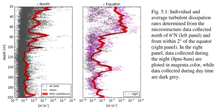
Fig. 5.1: Individual and average turbulent dissipation rates determined from the microstructure data collected north of 6°N (left panel) and from within 2° of the equator (right panel). In the right panel, data collected during the night (8pm-8am) are ploted in magenta color, while data collected during day time are dark grey.
In the upper 100m, the average turbulent dissipation rate was in the order of 3x10⁻⁷ m2s-3 for stations north of 6°N (Fig. 5.1). However, below 100m water depth, turbulence is weaker and its dissipation rate is mostly smaller than 10-8 m2s-3. In the vicinity of the equator, a decay with depth is even more evident. Turbulent dissipation rates regularly exceeded values of 5x10⁻⁶ m2s-3 within the upper 80m, but was several orders of magnitude weaker below that depth. In the upper equatorial ocean, a nighttime enhancement of turbulence was clearly observed.
5.5 Biochemical measurements 5.5.1 Tracermeasurements
(Tim Stöven, Sören Gutekunst)
During the cruise, a gas chromatographic - electron capture detector system was used in connection with a purge and trap unit (GC-ECD/PT5) for the measurements of the transient tracers CFC-12, SF6 and the deliberately released tracer CF3SF5. The system is a modified version of the set-up normally used for the analysis of CFCs (Bullister and Weiss, 1988). The PT5 instrument was used for measuring the transient tracers SF6 and CFC-12 as well as the released tracer CF3SF5
on all depths. Samples around the target density of the released tracer were taken with high volume ampoules of 1 L and the adjoining depths with syringes of 250 mL.
The trap consisted of 100 cm 1/16” tubing packed with 70 cm Heysep D kept at temperatures between -60 and -68°C during the purge and trap process. The traps were desorbed by heating to 110°C and injected onto a pre-column of 20 cm Porasil C followed by 20cm Molsieve 5A in a 1/8” stainless steel tubing. The main column consisted of 1/8” packed stainless steel tubing with 180 cm Carbograph 1AC (60-80 mesh) and a 50 cm Molsieve 5A post-column. All columns were kept isothermal at 50°C. Detection was performed on an Electron Capture Detector (ECD). This set-up allowed efficient and simultaneous analysis of all three tracers with some restrictions for CFC-12 due to the high sample volume in the target depth range.
The transient tracer samples were collected in 250 ml ground glass syringes, of which an aliquot about 200 ml was injected to the purge-and-trap system. The SF5CF3 samples were collected in
~1300 ml ampoules, of which an aliquot of ~990 ml was injected to the vacuum-sparge system by evacuating the purge chamber and then sucking in the water through an orifice.
Standardization was performed by injecting small volumes of gaseous standard containing SF6, SF5 and CFC-12. The company Dueste-Steiniger (Germany) prepared this working standard. The CFC-12 concentration in the standard has been calibrated vs. a reference standard obtained from R.F Weiss group at SIO, and the CFC-12 data are reported on the SIO98 scale. Another calibration of the working standard will take place in the lab after the cruise. Calibration curves were measured roughly once a week in order to characterize the non-linearity of the system, depending on workload and system performance. Point calibrations were always performed between stations to determine the short-term drift in the detector. Replicate measurements were taken on several stations for data statistics. The final processing and calibration of the obtained transient tracer data will be performed onshore at the GEOMAR in Kiel. At several stations along the 23°W section water samples for determination of HFCs, HCFCs and PFCs were flame-sealed in ~1300ml ampoules for measurement onshore at GEOMAR.
The fourth survey of the deliberately released transient tracer CF3SF5 showed a lateral distribution from south of Cap Verdi Islands down to 4°30’ N along the 23°W section. Eight depths around the target density covered the vertical distribution of the tracer patch within the control
volume. This provides additional information about the total amount of tracer remaining in the control volume and contributes to the preceding calculations on spreading rates and diffusion coefficients of the OMZ.
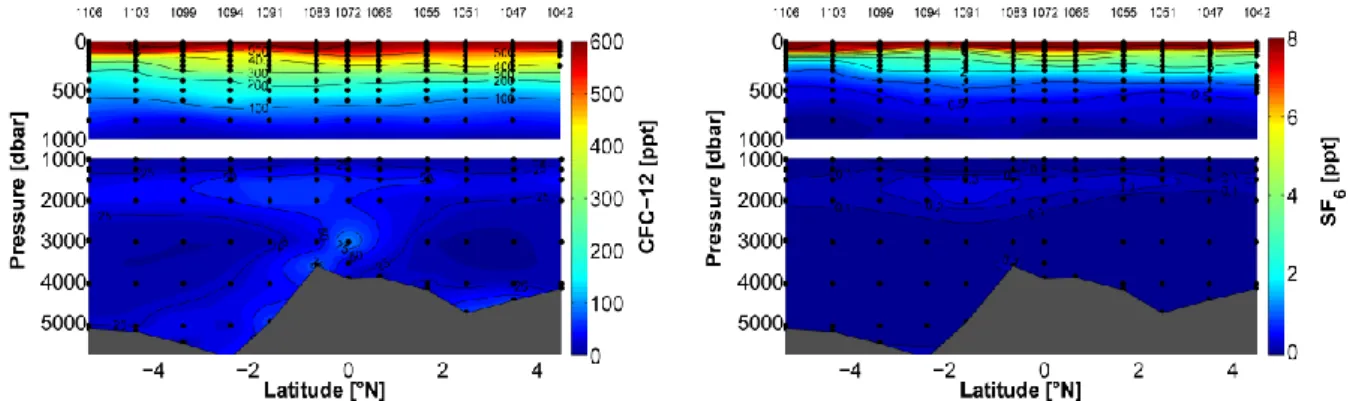
The distribution of CFC-12 and SF6 along 23°W and the two sections along the shelf break off Brazil describes the specific ventilation pattern of the different water masses (Fig. 3). The different distribution of both tracers is based on their different atmospheric histories so that CFC-12 already covers the deeper and less ventilated water masses. However, both tracers show a tracer maximum between 1800-2000 m originating from the Labrador Sea Water (LSW) situated in that depth range. The bottom water north of the mid-Atlantic ridge shows Denmark Strait Overflow water supplied by an eastward current whereas the elevated CFC-12 concentrations in bottom water south of the ridge indicate the cold and dens Antarctic Bottom Water (AABW). The two tracer sections along the Brazilian shelf break covering the boundary currents at ~5°S and 10°S were not processed until the end of the cruise.
All sections are an important contribution to the transient tracer data collection. The time series and repeat hydrography sections in the Atlantic Ocean allow for additional investigations on changes in ventilation and the adjoining parameters such as the anthropogenic carbon column inventory, i.e. the carbon uptake by the ocean, and the oxygen budgets in the ocean, especially in the oxygen minimum zones.
Fig. 5.2: Distribution of CFC-12 (left panel) and SF6 (right panel) partial pressure along 23°W.
5.5.2 Zooplankton ecology and particle dynamics (Rainer Kiko, Iris Kriest, Jannik Faustmann)
A Hydrobios® Multinet Midi with an aperture of 0.25 m2 and 5 net bags (mesh size 200 µm) was deployed at 7 daytime and 12 nighttime stations for vertically stratified hauls (sampling depths:
1000-600 m, 600-300 m, 300-200 m, 200-100 m, 100-0 m). Samples were fixed in 4%
formaldehyde in seawater solution. They will be scanned and analyzed in the home laboratory using automated imaging software allowing taxonomical classification and biomass estimation.
During 112 CTD casts, an UVP 5 (serial number 10) was operated on the CTD rosette. The instrument consists of one down-facing HD camera in a 6000 dbar pressure-proof case and two red LED lights, which illuminate a 0.88 L-water volume. During the downcast, the UVP takes 3- 11 pictures of the illuminated field per second. For each picture, the number and size of particles are counted and stored for later data analysis. Furthermore, images of particles with a size > 500 µm are saved as a separate “Vignettes” - small cut-outs of the original picture – which allow for later, computer-assisted identification of these particles and their grouping into different particle,
phyto- and zooplankton classes. Since the UVP was integrated in the CTD rosette and interfaced with the CTD sensors, fine-scale vertical distribution of particles and major planktonic groups can be related to environmental data.
During CTD casts and mooring work on 17 different stations a modified Working Party 2 (WP2) net was deployed by hand as a driftnet to collect different Rhizaria species from surface waters (1 to 5 m). Incubation experiments to determine respiration and NH4 excretion rates were conducted with the retrieved specimens at 18˚C and 23˚C. The collected organisms were scanned on an Epson Perfection V750 scanner to obtain size measurements and dried for later biomass analysis in the home laboratory. Additional 79 samples were collected for species identification via DNA analysis in the home laboratory.
5.5.3 Nutrient sampling and analysis
(Matthew Patey, Evangelia Louropoulou, Iris Kriest, Rainer Kiko)
Samples for inorganic nutrient and dissolved organic phosphorus were collected and frozen for transport to Kiel. Samples were also taken for dissolved nitrate + nitrite (NO2- and NO3-) (hereinafter nitrate) and dissolved phosphate (PO43-), at nanomolar concentration, and for dissolved ammonium (NH4+). Nanomolar nitrate and phosphate measurements were made on board using a purpose-built, segmented-flow autoanalyser following a method described in Patey et al. (2008) with some changes to reagent flow rates. Ammonium was measured using the OPA fluorescence method, as described by Holmes et al. (1999). Please note throughout this report molar concentrations are reported in concentrations per unit volume (i.e. nM, μM and mM refer to nmol l-1, μmol l-1, mmol l-1, respectively).
To determine nanomolar concentrations of nitrate and phosphate two liquid waveguide capillary flow cells (LWCCs) were used to provide a two-meter path-length, enabling the detection of nanomolar concentrations. A single tungsten-halogen lamp (HL2000-HP, Ocean Optics) provided illumination for both LWCCs, with a bifurcated fibre-optic cable being used to divide the light between the two channels. Two Ocean Optics USB spectrometers monitored the absorbance in each cell. Samples were introduced manually by switching a sample line between a reference solution (low nutrient surface seawater) and sample or standard solution and the resulting change in absorbance was monitored. Absorbance versus time was continuously recorded for each channel and stored electronically in a plain text format. Calibration curves and results were generated manually from the peak heights using spreadsheet software.
Ortho-phosphate is measured by formation of a blue reduced Molybdophosphate-complex at pH 0.9-1.1. Potassium Antimonyltartrate used as the catalyst and ascorbic acid as a reducing agent.
The absorbance is measured at 700 nm rather than the usual 880 nm due to low optical transmission at wavelengths longer than 700 nm (Murphy and Riley, 1962). Nitrate is first reduced in a copperized cadmium-coil using imidazole as buffer and is then measured as nitrite at 540 nm with reference correction using 700 nm (Grasshof, 1983).
Nanomolar concentrations of ammonium were determined by overnight incubation of 20 mL of sample with 2 mL of OPA reagent, prepared as described by Holmes et al. (1999). Standard additions were prepared using seawater taken from 600 – 1000 m depth and a 25 µM standard solution prepared from ammonium sulphate. Sample fluorescence were measured in a Trilogy Fluorometer equipped with an ammonium module and a 1 cm quartz cuvette. Data quality and consistency of the nanomolar nitrate and phosphate measurements was checked by daily monitoring of various parameters, including the Cu-Cd column reduction efficiency (for nitrate
measurements) and measurement of nutrient reference samples containing a stable nutrient concentration.
The sampling approach for nanomolar nitrate and phosphate, and ammonium included that all apparatus coming into contact with the samples or reagents were cleaned by soaking in 1M HCl and rinsing thoroughly with ultrapure water from a MilliQ system (hereafter referred to as MQ).
Samples were taken from the CTD rosette using 60 mL acid-washed LDPE bottles (nitrate and phosphate) and 50 mL polypropylene tubes (ammonium), rinsing three times before filling, and were stored in the fridge until analysis. Analysis was typically undertaken within 12 hours, although some samples collected during the night were not measured until the following afternoon (typically 18 – 20 hours later). For each CTD profile, typically 4 to 5 samples for nitrate and phosphate and 6 to 7 samples for ammonium were taken from the uppermost depths. Additionally, a number of surface samples were collected from a towed fish sampler.
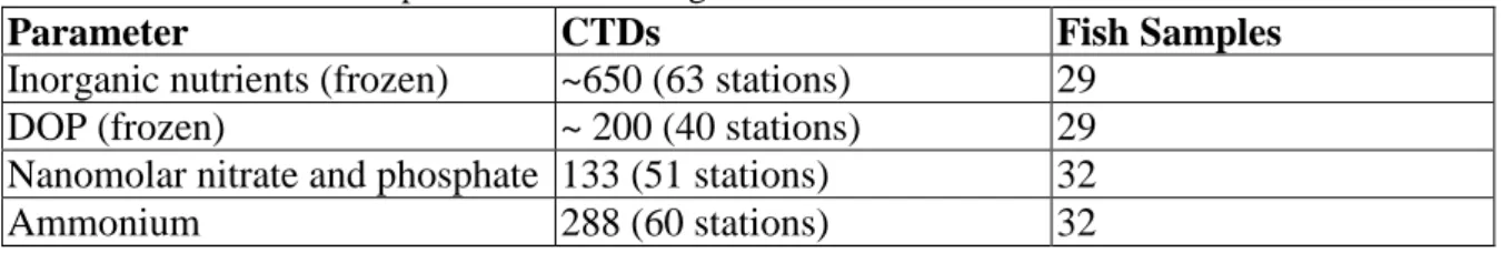
Samples from the CTD for dissolved organic phosphorus (DOP) and inorganic nutrients were sampled into 40 mL or 50 mL polypropylene tubes, rinsing three times before filling. Inorganic nutrient samples were frozen (-25 °C) immediately for transport to Kiel. DOP samples were first filtered using 0.2 µm cellulose acetate syringe filters before freezing (-25 °C). Samples from the towed fish sampler for DOP and inorganic nutrients were filtered directly using a Sartobran 0.2 µm filter and frozen for transport to Kiel. A total of 106 samples were measured from the underway system and 85 samples were taken from Niskin bottles (Table 5.4).
Table 5.4: Nutrient samples collected during M130.
Parameter CTDs Fish Samples
Inorganic nutrients (frozen) ~650 (63 stations) 29
DOP (frozen) ~ 200 (40 stations) 29
Nanomolar nitrate and phosphate 133 (51 stations) 32
Ammonium 288 (60 stations) 32
5.5.4 N2 fixation, primary productivity
(Ajit Subramaniam, Ana Fernández Carrera, Julia Dürschlag)
Size-fractionated N2 fixation and carbon uptake of the planktonic community were estimated following a dual 15N2 and 13C-bicarbonate tracer technique (Montoya et al. 1996) with water from 10 m at 36 stations (Table 7.4). In addition, “profile” measurements were made from three depths at seven stations. At each station, triplicate 4.4-L, clear polycarbonate bottles were filled directly from the CTD-rosette. After removing all air bubbles, 3 ml of 15N2 (98 atom%, SerCon) and 250 µL of 13C-bicarbonate were injected to each bottle. The 24-hour incubation was carried out on- deck in a system of re-circulating water simulating in situ photosynthetically active radiation levels, using neutral density screens/meshes. Particles for defining the natural abundance of carbon and nitrogen isotopes were collected at several sampling depth at each station by passing 1–15 L of water through pre-combusted 47 mm GF/F filters under gentle pressure. The abundance of carbon (C) and nitrogen (N) stable isotopes in incubated and natural abundance samples will be measured using the methods described in Montoya et al. (1996).
Samples were collected for analysis of High Performance Liquid Chromatography for estimating phytoplankton pigment concentrations from the upper 120m at 45 stations (Table 7.4).
Three liters of water were collected from 3-4 depths in the euphotic zone and filtered through a
GF/F filter. The filters were frozen in liquid nitrogen until analysis. The samples will be analyzed following the method of (Van Heukelem and Thomas 2001) at the NASA GSFC sample analysis facility. Samples were also collected from the same depths for enumerating bacterial, cyanobacterial, and picoeukaryote abundance and frozen in liquid nitrogen until analysis using a BD Influx Flowcytometer following the methods described in Duhamel et al. (2014).
The in-water light field was studied using a multichannel free falling spectroradiometer (Satlantic Micropro) that measured downwelling irradiance and upwelling radiance. A surface reference sensor mounted on the ship was used to measure the above water downwelling irradiance. This data was collected at 14 stations and was used to calculate the attenuation of light in the water column and depth of the euphotic zone.
Phytoplankton pigments were measured using Advanced Laser Fluorometry (ALF), a dual laser fluorescence sensor that was plumbed to the ship’s flow-through seawater system. This data was integrated with the ship’s GPS and thermosalinograph data to provide surface maps of chlorophyll concentration, a measure of phytoplankton abundance and phycoerythrin, a measure of cyanobacterial abundance. Profile measurements were also done using the ALF at 46 stations (Table 7.4).
In addition to the measurements described above, a total of 14 stations including three stations off the coast of Brazil (Table 7.2) were sampled for N2 fixation and primary production measurements (MPI-Bremen). A depth profile of four different depths were obtained; surface (10 m), above chlorophyll a maximum (Chl a max), Chl a max and below Chl a max. N2 fixation and primary production rates are determined through a 24h- incubation of collected seawater directly from the CTD with stable isotopes, i.e. 15N2 and 13C-bicarbonate, respectively. Incubations lasted 24 hours in on-deck incubators, which were kept at surface water temperature via seawater flow- through and were adjusted to three different light levels or kept in dark. The incubations were started in triplicate 4.7-L bottles by the addition of the stable isotopes using tested and recommended protocols (Klawonn et al. 2015) after methodological difficulties had been identified earlier (Mohr et al. 2010, Grosskopf et al. 2012, Wilson et al. 2012). After the 24-h incubation period, the seawater was filtered onto pre-combusted GF/F filters (0.7μm nominal pore size); the filters were frozen for later determination of the concentration of particulate organic carbon (POC) and particulate organic nitrogen (PON) as well as the carbon and nitrogen isotopic composition using an elemental analyser coupled to an continuous-flow isotope ratio mass spectrometer (EA-IRMS) at the Max-Planck-Institute for Marine Microbiology in Bremen.
For natural isotope abundance in particulate organic carbon and nitrogen at sampled depths, 4.7 L of seawater was filtered onto pre-combusted 25 mm GF/F filters. In addition, t0 samples was obtained from the respectively depth, which was filtered immediately on pre-combusted GF/F filter. Further, Chl a samples from the respectively depth were obtained.
In addition, also subsamples from the incubated samples will be selected for single-cell analyses of targeted organism to determine the individual activity of selected organisms as well as their contribution to total N2 fixation and primary production rates. Single-cell analyses will be carried out using a NanoSIMS 50L instrument located at the MPI Bremen. To clarify and study diazotrophic organisms, subsamples were transferred into glycerol to obtain isolates (not in Brazilian waters). Furthermore, samples for DNA and CARD-FISH analysis were collected (DNA not in Brazilian waters) by filtering of seawater through 0.22 µm polycarbonate filters The exact volumes were determined and recorded for each sample. CARD-FISH analyses were conducted