ORIGINAL ARTICLE
The Stability of Fe‑Isotope Signatures During Low Salinity Mixing in Subarctic Estuaries
Sarah Conrad1 · Kathrin Wuttig2,3 · Nils Jansen2,4 · Ilia Rodushkin5 · Johan Ingri1
Received: 28 January 2019 / Accepted: 5 October 2019 / Published online: 6 November 2019
© The Author(s) 2019
Abstract
We have studied iron (Fe)-isotope signals in particles (> 0.22 µm) and the dissolved phase (< 0.22 µm) in two subarctic, boreal rivers, their estuaries and the adjacent sea in northern Sweden. Both rivers, the Råne and the Kalix, are enriched in Fe and organic carbon (up to 29 µmol/L and up to 730 µmol/L, respectively). Observed changes in the particulate and dissolved phase during spring flood in May suggest different sources of Fe to the rivers during different seasons. While particles show a positive Fe-isotope signal during winter, during spring flood, the values are negative. Increased discharge due to snowmelt in the boreal region is most times accompanied by flushing of the organic-rich sub-surface lay- ers. These upper podzol soil layers have been shown to be a source for Fe-organic carbon aggregates with a negative Fe-isotope signal. During winter, the rivers are mostly fed by deep groundwater, where Fe occurs as Fe(oxy)hydroxides, with a positive Fe-isotope sig- nal. Flocculation during initial estuarine mixing does not change the Fe-isotope compo- sitions of the two phases. Data indicate that the two groups of Fe aggregates flocculate diversely in the estuaries due to differences in their surface structure. Within the open sea, the particulate phase showed heavier δ56Fe values than in the estuaries. Our data indicate the flocculation of the negative Fe-isotope signal in a low salinity environment, due to changes in the ionic strength and further the increase of pH.
Keywords Fe-isotopes · Fe geochemistry · Dissolved and particulate Fe · Organically complexed Fe · Fe(oxy)hydroxides · Salinity gradient · Spring flood
1 Introduction
Despite its high abundance in the continental crust (Wedepohl 1995), Fe can be the limit- ing element in a third of the ocean surface waters (Martin et al. 1991; Morel and Price 2003). Riverine Fe input is the main source of Fe to the oceanic Fe budget, and estuarine Electronic supplementary material The online version of this article (https ://doi.org/10.1007/s1049 8-019-09360 -z) contains supplementary material, which is available to authorized users.
* Sarah Conrad sarah.conrad@ltu.se
Extended author information available on the last page of the article
mixing controls how much Fe reaches the oceans (Wells et al. 1995; Raiswell and Canfield 2012). Particles and colloids in river water (ranging from 0.01 to 1 µm) flocculate into larger particles and aggregates due to the increased ionic strength within estuaries and then precipitate close to the shoreline (Boyle et al. 1977; Sholkovitz et al. 1978). These Fe parti- cles and colloids consist mainly of two forms, Fe-rich organic carbon (OC) compounds and Fe-rich (oxy)hydroxides (Ingri et al. 2006; Ilina et al. 2013; Kritzberg et al. 2014). The sur- face properties of these compounds vary as aggregates with OC have fewer mineral phases exposed at their surface (Eusterhues et al. 2008). The amount of mineral phases, in turn, affects their chemical reactivity during estuarine mixing, which for example is defined by size and speciation (Poulton and Raiswell 2005; Tagliabue et al. 2017). Hence, the river input of Fe into the ocean is substantially modified by flocculation processes that occur at the estuarine interface and dependent on the initial Fe phase (Eckert and Sholkovitz 1976;
Boyle et al. 1977; Sholkovitz 1978). Various studies showed the ability of OC to keep Fe in solution along the salinity gradient of an estuary (Krachler et al. 2010; Kritzberg et al.
2014). The aggregation, sedimentation and resulting burial of OC associated with Fe in estuarine environments have been described as the “rusty carbon sink” (Lalonde et al.
2012; Shields et al. 2016).
Earlier studies have addressed the possibility of using Fe-isotopes as a tool to identify water sources and to differentiate between Fe phases, i.e. Fe–OC complexes and Fe(oxy) hydroxides (Ingri et al. 2006; Escoube et al. 2009; Ilina et al. 2013; Poitrasson et al.
2014). In low-temperature environments, stable Fe-isotope mass varies about 6.0–8.0‰
in 56Fe/54Fe ratios (Dauphas et al. 2017; Wu et al. 2018), expressed as δ56Fe relative to the reference material IRMM-14 (Dauphas and Rouxel 2006; Rouxel and Auro 2010). The Fe- isotope values of Fe phases entering the ocean via rivers range between −1.2 and +1.8‰
(Conrad 2019 and references therein), and this variation has been used as a tool to map the contribution of Fe sources to the ocean on temporal and geographical scales (Conway and John 2015). For example, subarctic and temperate rivers supply Fe phases with a negative δ56Fe value to seawater (Ingri et al. 2006; Severmann et al. 2006; Escoube et al. 2009; Ilina et al. 2013). It has been shown that Fe-isotope fractionation strongly depends on redox reactions (Wiederhold et al. 2006) and the fractionation can be used to trace the Fe-isotope composition of different Fe phases at their origin (Ingri et al. 2006; Ilina et al. 2013; Dos Santos Pinheiro et al. 2014; Poitrasson et al. 2014). In arctic and subarctic rivers, filtration yields towards a separation of a heavy dissolved (δ56Fe of +0.43‰ ± 0.04‰) and a par- ticulate δ56Fe between −0.09 and +0.10‰ (Escoube et al. 2009).
In spite of their importance, the knowledge about the fate of different Fe aggregates during estuarine transport is small. The Fe-isotope composition of the Fe-OC aggregates has the potential to be used as a tracer for the cycling of Fe-OC aggregates during transport from land to the open ocean.
Over the last decades, Fe concentrations in boreal rivers draining into the Baltic Sea have been increasing continuously (Kritzberg and Ekström 2012; Sarkkola et al. 2013).
Changing redox conditions in organic-rich soils are most likely responsible for the elevated Fe concentrations (Kritzberg and Ekström 2012; Knorr 2013). Higher Fe concentrations lead to increasing coastal export and may have important implications for the receiving aquatic systems.
In this study, we combine the Fe-isotope data from the river mouth, estuary and open sea in a subarctic, boreal environment, to access which Fe phase is present at the varying locations. We show the seasonal variation of dissolved and particulate Fe-isotope ratios in two boreal rivers and their estuaries. Our study provides further information on the sea- sonal availability of different Fe complexes by the use of their Fe-isotope composition. The
hypothesis was, can the Fe-isotope ratio be used to trace different Fe complexes from the river mouths into the open ocean. Therefore, we address the following research questions:
(1) quantify the variation of Fe-isotope values at the river mouths and along their estuaries;
(2) identify processes leading to temporal changes; and (3) reveal the effect of salinity- induced mixing on the Fe-isotope ratio.
2 Materials and Methods 2.1 Sampling Site
For this study, water samples were collected in two rivers, their estuaries, and the adjacent sea in Northern Sweden (Fig. 1). The boreal rivers Kalix and Råne have their origin in the Caledonian Mountains and the Råne Träsk, respectively. Both river catchments consist of forest, wetlands and lakes (Online resources ESM_1; SMHI 2018). The main differ- ence is the size of their catchment with the Kalix’s being approximately seven times larger than the Råne’s catchment. Additionally, the catchment of the Kalix River contains about 11% mountainous area. Both rivers drain into the northernmost part of the Baltic Sea, the so-called Bothnian Bay (Fig. 1b). The Råne estuary is a semi-closed water-body, partly isolated by several islands. The Kalix estuary is more open to the Bothnian Bay and is a so-called salt wedge estuary (Holliday and Liss 1976), where freshwater floats on top of the denser seawater, with the freshwater layer getting thinner towards the sea. The Both- nian Bay and its catchment area (including the Kalix and Råne River) are ice-covered up to 6 months per year (Vihma and Haapala 2009). The catchment area is about 260,700 km2,
A
Bothnian Bay
Råne River Kalix River 70°N
65°N
60°N
55°N
65°N 66°N
10°E 20°E 30°E64°N21°E 22°E 23°E 24°E 25°E
0 m 50 m 750 m 500 m 400 m 300 m 200 m
50 m 100 m
100 m
B
maslmbsl
Kalix Estuary
Råne Estuary
{ {
Råne River catchment
Kalix River catchment
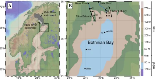
Fig. 1 A Overview map of Scandinavia and the Baltic Sea. The black dots display the sampling locations from five different sampling campaigns in Northern Sweden in 2013, 2014 and 2016. The dark and light grey areas mark the geographical locations of the Kalix and Råne River catchments, repectively. B Detailed map of the Bothnian Bay, with the sampling locations and their annotations. The two rivers Kalix (K1–4) and Råne (R1–4) drain into the Bothnian Bay (GOB1, GOB2, A5 and A13). Each station was sampled at three depths (0.5 m, 5 m and 10 m) if station depths allowed it. The legend on the right side of the maps shows metre above and below sea level (masl and mbsl, respectively). The Ocean Data View program, ver- sion 4.7.10 was used to generate the maps (Schlitzer, R., Ocean Data View, http://odv.awi.de, 2018)
and the high freshwater input and the low tide-influence lead to salinities below 4 (Kautsky and Kautsky 2000).
The boreal region has a subarctic climate, with extreme seasonal temperature varia- tions, with long, cold winters (− 20 to − 40 °C) and short, mild summers (20–30 °C), (Peel et al. 2007). Between 40 and 50% of the precipitation is snow (Ingri et al. 2005). With 5–7 months of winter, the moisture in the soils and subsoils freezes between 25 and 79 cm deep (Öquist and Laudon 2008; Haei et al. 2010). The river discharge has significant sea- sonal variations, and the main hydrological event is occurring in spring due to snow and ice melt (Fig. 2). There is an extended period of high discharge in the Kalix River, com- pared to the Råne River, resulting from snow and ice melt in mountainous regions (Fig. 2).
Discharge for both rivers was measured about 50 and 25 km upstream, respectively, at the stations Räktfors (Kalix River) and Niemisel (Råne River) by the Swedish Meteorological and Hydrological Institute (SMHI 2018).
For this study, the rivers, their estuaries and the Bothnian Bay were sampled during pre-flood, spring flood and post-flood (Table 1). Pre-flood samples were collected from beneath the ice-covered estuaries, in March 2014. Spring flood samples were collected in the estuaries and the Bothnian Bay in May and June 2013. Post-flood samples were col- lected in the Råne estuary and the Bothnian Bay in July 2014. In addition, pre-flood, spring flood and post-flood in Kalix and Råne River were sampled close to their river mouths between March and June 2016. The coordinates of each sampling location are summarized in the online resources (ESM_1).
2.2 Sampling and sample processing
All sampling stations were sampled at depths of 0.5, 5 and 10 m if they were deep enough (all except station K1 and R1). Water samples from the Kalix estuary, the Råne estuary and the Bothnian Bay were collected from the coast guard vessel KBV005 in May and June 2013. Four stations in each estuary (R1–R4 and K1–K4) and two stations in the Both- nian Bay (A5 and A13) were sampled. During the sampling in March 2014, samples were
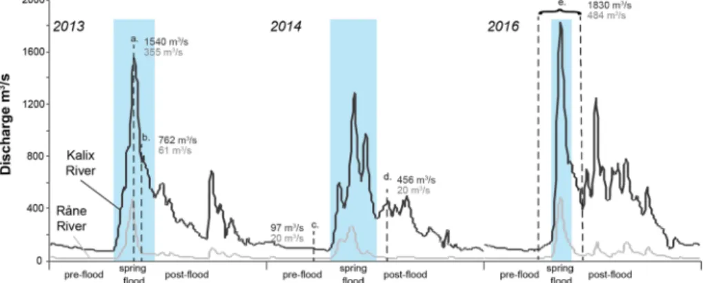
Fig. 2 Discharge from the Kalix (black) and Råne River (grey) during the sampling periods in 2013, 2014 and 2016 (SMHI). The dashed lines and letters indicate the five sampling events (a: 21–23 May 2013, b:
5–7 June 2013, c: 18 and 19 March 2014, d: 21 July 2014, and e: 25 March–15 June 2016). The discharge during each sampling is noted (for sampling event e, the maximum discharge during sampling is noted).
Below the x axis pre-flood, spring flood and post-flood are denoted for each year and the blue shaded areas mark the different spring flood events
obtained from the first three stations in the estuaries (R1–R3 and K1–K3), which were ice- covered. Details on the sampling in May and June 2013 and March 2014 can be found in Bauer et al. (2018). Briefly, the samples in 2013 were collected from the coast guard vessel KBV005 with 2 × 2 L Niskin bottles (Hydros-Bios, Kiel, Germany which had been custom- made trace metal clean containing only Ti screws, on a Dyneema rope, acid-cleaned 2-L LDPE bottles all parts acid cleaned) on a line in depths of 0.5, 5 and 10 m. In 2014, the samples were conducted through a hole in the ice, drilled with an ice auger and pumped up from the depths of 0.5, 5 and 10 m. During July 2014, the Råne estuary (R2) and two stations in the Bothnian Bay (GOB1 and GOB2) were sampled from the M/S Fyrbyggaren following the procedures and methods by (Cutter et al. 2010). Water samples were obtained with 5-L Niskin bottles (Hydros-Bios, Kiel, Germany) on a line in depths of 0.5, 5 and 10 m. Once retrieved, the bottles were emptied into sample acid-cleaned LDPE bottles, wrapped in polyethylene bags. Salinity, temperature, pH, alkalinity and dissolved oxygen were monitored with a Hydrolab Multisonde 5 (Online resources ESM_1). The sampling stations in the Kalix River, Kamlunge, and in the Råne River, Orrbyn, were partly ice- covered until early May 2016. Samples were collected from a bridge in the middle of each river. Specific conductivity, temperature, pH and dissolved oxygen were monitored with a Hydrolab Multisonde 5 (Online resources ESM_1).
All materials in contact with samples consisted of LDPE and were acid cleaned (1.1 M HNO3; Merck Millipore pro analysis EMSURE), before and between samplings (Ödman et al. 1999). All water samples were filtered within 6 h through 0.22 -µm pore Table 1 Sampling stations and their sampling occasions
The sample notations are assembled by the station name and the sampling event (a: May 2013; b: June 2013; c: March 2014; d: July 2014; e: March to June 2016). Information on the flow environment can be found for each sampling
Station Estuaries and Bothnian Bay Rivers
Spring flood Pre-flood Post-flood Pre-flood Spring
flood Post-flood May 2013 Jun 2013 Mar 2014 Jul 2014 Mar–Jun 2016
Råne Estu-
ary R1 R1a R1b R1c – – – –
R2 R2a R2b R2c R2d – – –
R3 R3a R3b R3c – – – –
R4 – R4b – – – – –
Kalix
Estuary K1 K1a K1b K1c – – – –
K2 K2a K2b K2c – – – –
K3 K3a K3b K3c – – – –
K4 K4a K4b – – – – –
Bothian
Bay A5 A5a A5b – – – – –
A13 A13a A13b – – – – –
GOB1 – – – GOB1d – – –
GOB2 – – – GOB2d – – –
Råne
River RR – – – – RR1e–
RR3e RR4e–
RR9e RR10e–
RR13e Kalix
River KR – – – – KR1e–
KR3e KR4e–
KR9e KR10e–
KR13e
size membrane filters (Merck MF-Millipore Membrane Filter, mixed cellulose esters, hydrophilic, diameter 142 mm), which were locked in polycarbonate filter holders under a clean bench with a peristaltic pump, yielding into a particulate (PFe > 0.22 µm) and a dis- solved (DFe < 0.22 µm) fraction. Membrane filters were cleaned with ultrapure acetic acid (99–100%) and stored in Milli-Q ultrapure water (18.2 MΩ cm at 25 °C) before they were used. The filtered water was acidified with ultrapure distilled 10% HNO3 to a pH below 2 and stored at 4 °C. The filters were stored in petri dishes at −18 °C until analyses.
Furthermore, water samples from 2016 were filtered through 0.7-µm glass fibre filters (GF/F Whatman®) for dissolved and particulate organic carbon analyses (DOC and POC).
The filters were pre-combusted for four hours to limit the C blanks (Brodie et al. 2011).
The filters for POC analyses were stored at − 18 °C before analyses by UC Davis Stable Isotope Facility (USA).
3 Analytical Methods
All samples were analysed for elemental composition and Fe-isotope composition in col- laboration with ALS (Australian Laboratory Services) Scandinavia AB, Luleå, Sweden.
All sample manipulations were performed in a clean laboratory (Class 10,000) by person- nel wearing clean room gear and following all general precautions to reduce contamination (Rodushkin et al. 2010). High-purity Suprapure® acids were used throughout sample treat- ment and analyses. Accredited DOC analyses were determined at the Umeå Marine Sci- ences Centre (Samples 2013 and 2014) and ALS Scandinavia (Samples 2016).
3.1 Element Concentration by Inductively Coupled Plasma Sector Field Mass Spectrometry (ICP‑SFMS)
For the elemental composition, the dissolved samples were diluted (2–200 fold) in 2.2 M HNO3; the degree of dilution depended on the salinity of the sample. The filters were treated with 10 mL of a 1000:1 mixture of HNO3/HF overnight followed by closed-vessel digestion in a microwave oven (600 W, 1 h). An aliquot of the digests was further diluted in 2.2.M HNO3 by the factors of 5 and 50 (2016 and 2013/2014, respectively) for the determi- nation of Fe concentrations.
Multi-elemental analyses (i.a. Fe, Rb, Sr) were performed in the dissolved and particu- late phases of the samples by ICP-SFMS (ELEMENT XR, Thermo Scientific, Bremen, Germany). A combination of internal standardization (indium added at 2 µgL−1 to all measurement solutions) and external calibration verified the measurements. All measured data fall within a 4-point calibration curve. Details of the analytical procedure as well as instrument parameters and analysis conditions can be found elsewhere (Rodushkin and Ruth 1997; Rodushkin et al. 2005). The analytical procedure was validated with SLRS-4 River Water CRM for Trace Metals, SLEW-2 Estuarine Water CRM for Trace Metals and NASS-4 open ocean water (supplied by National Research Council, Ottawa, Canada), (Rodushkin et al. 2005, 2016). Fe was analysed on three different instrument runs with an average detection limit (LOD) of 14 nM for the dissolved samples and 21 nM for the par- ticulate samples taken in 2013 and 2014 (LOD = Xbl + 3SDbl, Xbl = mean concentration of Fe in blanks; SDbl = Standard deviation of blanks). Replicated measurements showed a pre- cision of ± 1.3% (n = 8) for the particulate phase and ± 3.0% (n = 3) for the dissolved phase.
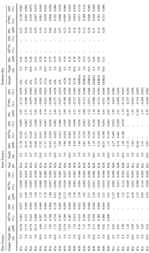
Table 2 Iron concentrations and Fe-isotope data for samples taken in the Kalix and the Råne estuary and the Bothnian Bay in 2013 and 2014 Råne EstuaryKalix EstuaryBothnian Bay SampleDepth (m)DFe (μM)Dδ56Fe (‰) 2SD (‰)
PFe (μM)Pδ56Fe (‰)
2SD (‰)
Sam- pleDepth (m)DFe (μM)Dδ56Fe (‰)
2SD (‰)
PFe (μM)δ56PFe (‰)
2SD (‰)
SampleDepth (m)DFe (μM)Dδ56Fe (‰)
2SD (‰)
PFe (μM)δ56PFe (‰)
2SD (‰)
R1a0.516.260.4840.0714.51− 0.0280.035K1a0.517.300.4200.0594.07− 0.1230.039A5a0.50.26––0.350.1200.062 R1a5.015.330.3250.0306.49− 0.0440.018K1a5.016.550.3710.0622.75− 0.0860.053A5a5.00.28––0.300.0910.064 R2a0.510.760.4420.0582.26− 0.0530.034K2a0.516.490.4360.0324.31− 0.0790.040A5a10.00.28––0.340.1050.072 R2a5.010.330.4000.0283.49− 0.0240.038K2a5.018.680.4110.0405.82− 0.0830.042A13a0.50.22––0.290.0870.074 R2a10.04.660.3870.0401.71− 0.0690.062K2a10.017.920.4110.0434.04− 0.0850.028A13a5.00.20––0.160.0810.040 R3a0.57.110.3290.0682.78− 0.0200.008K3a0.517.170.4490.0475.79− 0.0210.022A13a10.00.19––0.120.0780.042 R3a5.07.050.3400.0661.80− 0.0570.050K3a5.016.630.4540.0384.11− 0.0960.048A5b0.50.75––0.660.0460.028 R3a10.01.720.3180.1280.42− 0.0650.052K3a10.011.910.4250.0822.84− 0.1270.038A5b5.00.79––0.610.1020.006 R1b0.514.040.3870.04215.49− 0.0440.062K4a0.55.690.4120.0660.37− 0.0770.034A5b10.00.62––0.570.0860.016 R1b5.013.540.3660.05012.23− 0.0300.032K4a5.05.680.4260.0582.04− 0.1080.028A13b0.50.10––0.22− 0.0950.066 R2b0.57.070.4870.0942.260.0650.024K4a10.05.000.4030.0501.61− 0.0840.046A13b5.00.10––0.190.0550.028 R2b5.07.160.4140.0582.360.0620.062K1b0.58.490.2200.0484.33− 0.1270.094A13b10.00.10––0.180.0540.028 R2b10.06.360.4350.0222.580.0910.046K1b5.01.880.3140.0761.52− 0.0350.042GOB1d0.50.20––0.180.6710.154 R3b0.57.270.3990.0303.820.0020.026K2b0.58.630.2760.0524.00− 0.1110.046GOB1d5.00.14––0.320.4890.110 R3b5.07.180.4340.0482.37− 0.0150.050K2b5.05.590.3380.0323.12− 0.0710.008GOB1d10.00.25––0.280.6080.068 R3b10.06.730.3900.0362.20− 0.0110.006K2b10.01.290.3210.2361.16− 0.0860.034GOB2d0.50.04––0.310.5490.058 R4b0.59.080.4690.0483.82− 0.0250.048K3b0.58.240.4490.0464.49− 0.1230.054GOB2d5.00.05––0.140.5830.094 R4b5.09.020.4880.0443.31− 0.0350.040K3b5.010.510.3990.0544.01− 0.0710.048GOB2d10.00.11––0.200.5330.086 R4b10.07.250.4900.0443.07− 0.0220.030K3b10.01.330.1560.0440.97− 0.1080.028 R1c0.58.65––13.320.0810.058K4b0.58.270.4840.0321.950.0150.086 R1c5.00.91––0.800.0710.046K4b5.06.340.4810.0302.91− 0.0560.036 R2c0.53.90––3.220.1220.054K4b10.01.400.1080.0701.10− 0.1240.032 R2c5.01.28––0.730.0490.072K1c0.513.29––10.390.1970.050 R2c10.00.50––0.460.0210.050K1c5.02.69––1.55− 0.0150.058 R3c0.53.67––2.520.0980.052K2c0.510.46––11.380.1740.050 R3c5.01.03––0.950.1410.054K2c5.02.33––1.37− 0.0500.052 R3c10.00.52––0.540.0480.048K2c10.00.83––0.55− 0.0490.062
Table 2 (continued) Råne EstuaryKalix EstuaryBothnian Bay SampleDepth (m)DFe (μM)Dδ56Fe (‰) 2SD (‰)
PFe (μM)Pδ56Fe (‰)
2SD (‰)
Sam- pleDepth (m)DFe (μM)Dδ56Fe (‰)
2SD (‰)
PFe (μM)δ56PFe (‰)
2SD (‰)
SampleDepth (m)DFe (μM)Dδ56Fe (‰)
2SD (‰)
PFe (μM)δ56PFe (‰)
2SD (‰)
R2d0.50.15––0.650.3160.062K3c0.510.74––11.420.2090.072 R2d5.00.22––0.850.3780.066K3c5.02.06––1.43− 0.0920.090 R2d10.00.34––0.530.3580.068K3c10.00.73––0.700.2610.118
The average detection limit for both phases in 2016 was 9 nM and replicated measurements showed a precision of ± 4.5% (n = 41).
3.2 Iron Isotope Ratio Measurements by MC‑ICP‑MS
For the Fe-isotope measurements, an aliquot of the dissolved samples and the digested fil- ters was evaporated. Depending on the Fe concentration, 50 and 1000 ml of sample solu- tion was evaporated. The residuals were re-dissolved in 1 mL 8 M HCl. Iron was sepa- rated from the matrix elements by using an AG-MP-1 M ion-exchange resin (microporous, 100–200 mm dry mesh size, 75–150 mm wet bead size, Bio-Rad Laboratories AB, Solna, Sweden). After the sample was loaded, the matrix was washed with 9.6 M HCl, and Cu was eluted with 8 ml 5 M Cl. Afterwards, Fe was eluted with 6 ml 2 M HCl and could be used for further steps (Rodushkin et al. 2016). After evaporating to dryness, 50 µL of con- centrated HNO3 was pipetted directly to the residue followed by the addition of 5 mL MQ- water. Samples with high Fe content were diluted with 0.2 M HNO3 to a concentration of 2 mg L−1 in the measurement solutions. Low Fe concentration water samples were fur- ther diluted to 0.7–0.9 µmol/L and measured using high-efficiency desolvation nebulizer (Aridus) in a separate analytical sequence. Iron was separated from the matrix by this ion exchange with a yield of > 95%.
Fe-isotope ratio measurements were performed on a multi-collector inductively coupled plasma mass spectrometer (MC-ICP-MS, NEPTUNE and NEPTUNE PLUS) in high-reso- lution static mode relative to IRMM-14 CRM. The 54(Fe and Cr), 56Fe, 57Fe, 58(Fe and Ni),
60Ni and 62Ni were collected by the eight adjustable Faraday cups of the NEPTUNE. The instruments were equipped with a micro-concentric nebulizer and tandem cyclonic/Scott Table 3 Iron concentrations and Fe-isotope data for the Kalix and the Råne River sampled in 2016
DFe (µM) Dδ 56Fe (‰) 2σ (‰) PFe (µM) Pδ56Fe (‰) 2σ (‰) Kalix River
KR2e 8.0 0.587 0.048 6.6 0.239 0.104
KR4e 9.0 0.483 0.050 8.9 0.149 0.052
KR5e 13.4 0.472 0.132 8.1 0.004 0.128
KR6e 13.5 0.472 0.102 11.2 − 0.025 0.132
KR7e 11.6 0.494 0.050 11.0 − 0.018 0.050
KR9e 6.7 0.576 0.050 5.0 − 0.064 0.080
KR10e 6.5 0.496 0.098 4.6 − 0.059 0.114
KR13e 5.1 0.521 0.060 4.3 0.068 0.080
Råne River
RR2e 11.3 0.615 0.044 13.1 0.302 0.058
RR4e 14.1 0.543 0.048 14.1 0.227 0.064
RR5e 14.2 0.549 0.082 12.2 0.127 0.070
RR6e 13.3 0.551 0.076 20.3 0.190 0.058
RR7e 11.0 0.545 0.104 18.4 0.047 0.096
RR9e 9.4 0.589 0.050 11.7 0.017 0.056
RR10e 7.6 0.589 0.044 9.0 − 0.072 0.152
RR13e 7.2 0.477 0.048 7.9 − 0.012 0.096
double-pass spray chamber. Instrumental mass biases were corrected by sample-standard bracketing using IRMM-14 CRM, while an internal standard (Ni) was added to all samples and used to correct for instrumental drift. The online data correction considered baseline subtraction (120 s before each measurement), calculation of ion beam intensity ratios and filtering of outliers by a 2σ test. Detailed information on the correction procedures can be found in Baxter et al. (2006).
Iron isotope data are expressed as δ56Fe, relative to the IRMM-14 standard.
In-house quality control samples (prepared by sequential dilutions of SPECTROSCAN 10,000 mg L−1 Fe element standard for atomic spectroscopy from TEKNOLAB, Drøbak, Norway) were analysed at the beginning and the end of each analytical session to ensure internal consistency of the analytical results. Each analysis was made as a sequence of standard, three samples, standard. All samples and standards were analysed in duplicates, and the internal analytical precision was better than ± 0.01% [± 2 standard deviations (SD)].
Fe-isotope ratios in this material were measured on a regular basis at ALS laboratory from 2003, and a mean δ56Fe of − 0.24 ± 0.03 ‰ (n > 120, one sigma) makes it a suit- able reproducibility control for Fe-isotope ratio measurements in low fractionated samples (Baxter et al. 2006). Within the analysed samples, the δ56Fe values were reproduced with a standard deviation of 8.03% for the particulate phase and 2.50% for the dissolved phase in 2013/2014. In 2016, iron isotope data in both phases were reproduced with a precision of 2.7%. In the three-isotope plot of δ56Fe and δ57Fe, all samples plot on a single-mass fractionation line similar to the theoretical kinetic fractionation line (Young et al. 2002;
Kavner et al. 2005), which shows the robustness of the measurements (Online resources ESM_2). In this study, we only discuss the δ56Fe, δ57Fe data which are reported in the online resources (ESM_1) including their errors (2SD).
4 Results 4.1 Spring Flood
The peak discharge in the Kalix River was about 3–4 times higher than in the Råne River (Fig. 2). The pH in the Kalix and the Råne River varied between 5.6 and 6.9 with no clear correlation to the discharge (ESM_2, Fig. S2). Within the estuaries, the pH was increas- ing with distance to the shoreline in both estuaries and showed little variation with depths (from 6.5 to 7.4). pH in the Bothnian Bay showed little variation between 7.7 and 7.9 (ESM_2, Figs. S3 to S5).
The salinity generally increased with distance to the shore and with depths (ESM_2, Fig. S3 to S5). The salinity at the northernmost station (A5) was about 0.5 points lower than at station A13 during late spring flood (2.5 and 2.9, respectively).
The DOC and POC concentrations in both rivers increased with increasing discharge (ESM_2, Fig. S2). DOC concentration ranged from 500 to 740 µmol/L, while POC ranged from 71 to 134 µmol/L. The high DOC concentrations were also found in the estuaries.
Overall, the DOC concentration decreased with distance to the shore, and the variations δ56Fe(‰) =
[ (56
Fe∕56Fe)
sample
(56
Fe∕56Fe)
IRMM-14
−1 ]
∗103
with depths were negligible (411–718 µmol/L) (ESM_2, Fg S3 and S4). In the Kalix estuary, during spring flood, the DOC concentration increased with distance to the shore (K1–K3) and then decreased towards station K4. During late spring flood, in the Kalix estuary, there is an overall increase towards the sea. In the Råne estuary, the DOC concen- tration was decreasing from land to sea (ESM_2, Fig. S4). The DOC concentration in the Bothnian Bay was homogenous between 348 and 396 µmol/L. Station A5 had the highest DOC concentrations within the Bothnian Bay during late spring flood (ESM_2, Fig. S5).
Both rivers showed a large increase in DFe and PFe concentration during the spring flood (Fig. 3; Table 2). The main increase in DFe occurred before the maximum discharge of the season, increasing from 5 and 14 µmol/L. Dissolved Fe concentrations measured in the Råne River were slightly higher than in the Kalix River. Particulate Fe increased later, compared to the DFe, with values ranging from 4 to 20 µmol/L.
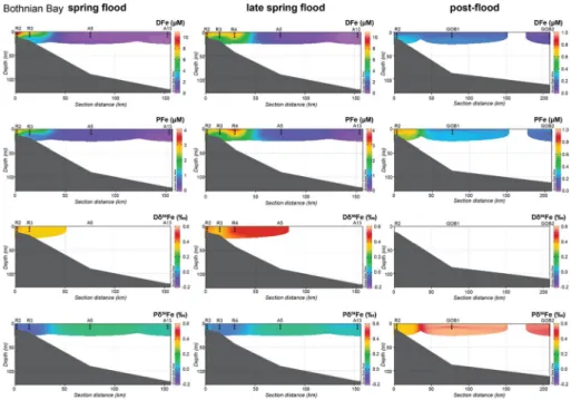
Riverine Fe input varies throughout the year and influences the Fe distribution along the estuaries and in the Bothnian Bay. The DFe concentration in the Kalix and Råne estuaries decreased with increasing salinities towards the open Bothnian Bay (Figs. 4, 5, Table 3). At most stations, the DFe concentration also decreased with depths as salinity increased. Dur- ing spring flood, DFe in the Kalix estuary varied between 18.7 and 1.4 µmol/L. In the Råne estuary, the DFe concentration varied between 1.7 and 16.3 µmol/L (Fig. 5) with the lowest concentrations at depths of 10 m, where the salinities were comparably high. During late spring flood, the DFe concentration was slightly lower, but the decrease in DFe with depths was less distinct (6.4–14 µmol/L). Within the Bothnian Bay at salinities around 3 g/kg, the DFe concentration ranged from 0.1 to 0.8 µmol/L with little variation in depth (Fig. 6). The highest concentrations occurred at station A5 in June. Along both estuaries, the depths pro- files suggest decreasing PFe concentrations from land to sea, but the trend was not as clear as in the dissolved fraction. In general, the PFe concentration decreased with depths. In the Kalix estuary, the PFe concentration ranged from 0.4 to 5.8 µmol/L during the spring flood. In the Råne estuary, the measured PFe concentration ranged from 0.4 to 6.5 µmol/L, whereas station R1 showed exceptional high PFe concentrations of 15.5 µmol/L. Partic- ulate Fe in the open Bothnian Bay showed little variation between 0.1 and 0.7 µmol/L, whereas the highest concentrations occurred at station A5 during June (Fig. 6).
All Fe-isotope compositions in the particulate and the dissolved phase are relative to the reference material IRMM-14. Our data fall within Fe-isotope ratios described for the boreal and arctic regions [Dδ56Fe: −1.2 to +1.8‰; Pδ56Fe: −1.0 to +0.6‰; (Ilina et al.
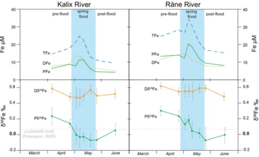
2013; Escoube et al. 2015; Zhang et al. 2015; Opfergelt et al. 2017)]. Within the rivers, the Dδ56Fe values varied between +0.47 ± 0.10 and +0.59 ± 0.05‰ in Kalix River and between +0.48 ± 0.05 and +0.62 ± 0.04‰ in Råne River (Fig. 3). The Pδ56Fe values ranged from +0.24 ± 0.10 to −0.06 ± 0.08 in Kalix River and from +0.30 ± 0.06 to −0.07 ± 0.15‰
in Råne River. The DFe-isotope composition was at all times higher than the PFe-isotope values. The Dδ56Fe composition showed small variations during the season, while the Pδ56Fe composition, in both rivers, was more negative during spring flood. Between the two phases, a difference of minimum 0.3‰ points and a maximum of about 0.7‰ points were measured. There was a significant difference of 0.40‰ in the results for DFe (average 0.54‰; SD = 0.05‰) and PFe (average 0.07‰; SD = 0.12‰); p < 0.001, n = 30.
During spring flood, the DFe in the Kalix and Råne estuaries showed positive δ56Fe values, which varied from +0.11 ± 0.07 to +0.48 ± 0.03‰ and from +0.32 ± 0.13‰ to +0.49 ± 0.04‰, respectively (Figs. 4, 5). Overall the transect profiles showed little var- iation with depths, the most distinct change occurs in the Kalix estuary between 5 and 10 m depth, with a shift from +0.40 to +0.16‰ (K3) and from +0.48 to +0.11‰ (K4) during late spring flood. The Fe-isotope composition of PFe showed negative values on
Fig. 3 Variation in Fe concentration and Fe-isotope composition in Kalix (left) and Råne River (right). The total Fe (TFe) concentration is calculated as the sum of DFe and PFe. The shaded area indicates the spring flood. Fe-isotopes are displayed as δ56Fe relative to the IRMM-14 standard material. The errors are pre- sented as 2SD
Fig. 4 Kalix estuary concentration transects for DFe (first row) and PFe (second row), as well as the Dδ56Fe (third row) and Pδ56Fe (fourth row) isotope composition. The stations were sampled during pre-flood, spring flood and late spring flood. The Ocean Data View program, version 4.7.10, was used to generate the transects (Schlitzer, R., Ocean Data View, http://odv.awi.de, 2018)
the average and little variation with depths. Within the Kalix estuary, the δ56Fe of PFe ranged from −0.13 ± 0.04 to +0.02 ± 0.09‰. The Pδ56Fe in the Råne estuary tended to be slightly more positive and ranged from −0.07 ± 0.06 to +0.09 ± 0.05‰. The Pδ56Fe within the Bothnian Bay showed little variation with an average of +0.07 ± 0.04‰. There was a significant difference of 0.44‰ in the results for DFe (average 0.39‰; SD = 0.09‰) and for PFe (average − 0.05‰; SD = 0.05‰); t(41) = 2.59, p = 0.011. Escoube et al. (2009) reported a difference between the two phases of 0.50‰.
4.2 Pre‑flood and Post‑flood
During pre-flood, discharge in the Kalix River is four to five times higher than in the Råne River. During post-flood on the other hand, the discharge of the Kalix River is about 23 times higher, due to the delayed snowmelt from the mountains in the catchment of the Kalix River (Fig. 2). The salinity in the estuaries during pre-flood varied between 0 and 2.6 g/kg (ESM_1 and _2), whereas just the surface water samples had salinities around 0 g/
kg, the deeper samples had values between 1.7 and 2.6 g/kg. During post-flood, the water column in the Råne estuary (R2) was well mixed and showed an average salinity of 2.4 g/
kg (ESM_1 and _2). The water column in the Bothnian Bay was well mixed with an aver- age salinity of 3.2 g/kg. Dissolved OC concentrations were lowest in the rivers and estuar- ies during base flow conditions (242–552 µmol/L) (ESM_2). During pre-flood, the DOC concentrations in the Kalix estuary were lowest in the surface samples (293–303 µmol/L), and values increased with depths to 415 µmol/L. In the Råne estuary, DOC concentrations Fig. 5 Råne estuary concentration transects for DFe (first row) and PFe (second row), as well as the Dδ56Fe (third row) and Pδ56Fe (fourth row) isotope composition. The stations were sampled during pre-flood, spring flood and late spring flood. The Ocean Data View program, version 4.7.10, was used to generate the transects (Schlitzer, R., Ocean Data View, http://odv.awi.de, 2018)
at the water surface were higher (425–469 µmol/L) compared to the deeper waters (328 µmol/L) (ESM_2), the concentrations were similar during pre- and post-flood. Within the Bothnian Bay, the DOC varied between 117 and 393 µmol/L, with decreasing concen- trations southwards. The DOC in these profiles increased with depth (ESM_2, Fig. S5).
During pre-flood, the DFe concentration varied between 0.2 and 13.2 µmol/L for both estuaries (Figs. 4, 5). The surface samples had very high concentrations (average 8.5 µmol/L) compared to the underlying water column (average 1.3 µmol/L). During post- flood, the DFe concentrations in the Råne estuary showed little variation with an average of 0.2 µmol/L (Fig. 6). The concentrations in the Bothnian Bay showed little variation around 0.1 µmol/L (Fig. 6). The surface waters sampled during pre-flood showed very high PFe concentrations (up to 13.3 µmol/L) values compared to the underlying water (on average 0.8 µmol/L). During post-flood, the PFe concentration in the Råne estuary ranged from 0.5 to 0.9 µmol/L. Samples from the Bothnian Bay after spring flood showed little variation between 0.1 and 0.3 µmol/L.
No dissolved Fe-isotope data are available for pre- and post-flood. The δ56Fe compo- sition of the PFe in the estuaries showed no clear trend during pre-flood (Figs. 4, 5). In the Kalix estuary, the Pδ56Fe ranged from −0.09 ± 0.09 to +0.21 ± 0.07‰, whereas just the surface water samples had a positive Fe-isotope composition. In the Råne estuary, the Pδ56Fe ranged from +0.02 ± 0.05 to +0.14 ± 0.05‰ pre-flood and from +0.32 ± 0.06 to +0.38 ± 0.07‰ post-flood conditions. Within the Bothnian Bay during post-flood, the Pδ56Fe composition ranged from +0.48 ± 0.11 to +0.67 ± 0.15‰.
Fig. 6 Bothnian Bay concentration transects for DFe (first row) and PFe (second row), as well as the Dδ56Fe (third row) and Pδ56Fe (fourth row) isotope composition. The stations were sampled during spring flood and late spring flood and post-flood. For reference data, the transects start at station R2 in the Råne estuary. The Ocean Data View program, version 4.7.10, was used to generate the transects (Schlitzer, R., Ocean Data View, http://odv.awi.de, 2018)
5 Discussion
5.1 Temporal Variations of Fe
Seasonal dynamics in the boreal region suggest varying hydro-geological pathways throughout the year (Dahlqvist et al. 2007; Rosenberg and Schroth 2017). During pre-flood, low Fe and DOC concentrations, as well as high pH values, indicate groundwater as source for riverine input (Dahlqvist et al. 2007; Wortberg et al. 2017). In boreal regions, up to 2/3 of the annual discharge is transported during the spring flood (Pontér et al. 1990; Lidman et al. 2011). Increased discharge has a significant influence on the chemical composition of rivers, estuaries and the open sea. During spring flood, increasing DOC, Fe and decreas- ing pH suggest the inflow from organic-rich soil layers into the rivers (Seibert et al. 2009;
Ledesma et al. 2015; Ingri et al. 2018). The riparian zone and its organic-rich soil layers are the main source for the increased DOC and Fe in subarctic, boreal forest rivers dur- ing the snow melt and the associated spring flood (Laudon and Bishop 1999; Bishop et al.
2004; Grabs et al. 2012). Recently, the flushing of the upper soil horizons in the catchment of the Kalix River has been validated with the use of the Rb/Sr ratio and Sr-isotope ratio by Wortberg et al. (2017). Our data show a clear correlation between the Pδ56Fe composition and the Rb/Sr ratio (R2 = 0.75), with positive Pδ56Fe values corresponding with low Rb/
Sr ratios, whereas a negative Pδ56Fe composition corresponds with the high Rb/Sr ratio—
the identified flushing component. This correlation implies that the origin of a negative δ56Fe composition is lying within the upper soil layers, available due to flushing events.
The decrease in Pδ56Fe values from +0.24 to −0.06‰ in the Kalix River and from +.30 to −0.07‰ in the Råne River reflects the changing hydro-geological pathways between pre-flood and spring flood for PFe. The Dδ56Fe composition, on the other hand, is almost stable with an average composition of +0.53 ± 0.05‰ throughout pre-flood, spring flood and post-flood, indicating no or little variation of the DFe source.
In boreal regions, Fe is transported in two primary forms in the rivers: Fe-OC complexes and Fe (oxy)hydroxides (Ilina et al. 2013; Neubauer et al. 2013; Sundman et al. 2014). In arc- tic and subarctic rivers, the high DOC concentration leads to the building of organo-mineral colloidal status for most metals, i.e. Fe (Pokrovsky et al. 2010; Schroth et al. 2011; Ingri et al.
2018). Organic carbon can stabilize Fe aggregates during transport (Kritzberg et al. 2014;
Herzog et al. 2017). Salinity-induced aggregation experiments in both rivers resulted in an aggregated phase dominated by Fe(oxy)hydroxides with a lower Fe-isotope composition than the remaining suspended phase, with a higher amount of Fe-OM (Herzog et al. 2019). There- fore, we assume that DFe is dominated by Fe-OM complexes with positive Fe-isotope values, while PFe seems to be dominated by Fe(oxy)hydroxides with lower δ56Fe. Evidence suggests that the decrease in Pδ56Fe is caused by the input of negative Fe-OC complexes from organic- rich surface soils, flushed during spring flood. The comparable heavier values during pre- and post-flood origin from Fe(oxy)hydroxides precipitated from anoxic groundwaters with high amounts of dissolved Fe(II) concentrations (Neubauer et al. 2013). Boreal first-order streams have mainly Fe-OC complexes, where the Fe occurs in the reduced Fe(II) or a mixed Fe(II)/
Fe(III) oxidation states (Emmenegger et al. 1998; Rose and Waite 2003; Sundman et al. 2013), the higher-order streams consist of Fe-OC complexes and nanoparticulate Fe(oxy)hydrox- ides, which aggregate and can be found in the > 0.22 µm fraction (Neubauer et al. 2013). With the decreasing amount of Fe-OC complexes, the amount of Fe(oxy)hydroxides with Fe(III) increases (Lofts et al. 2008; Neubauer et al. 2013).
Summarizing, we suggest that the DFe reaching the estuaries has a relatively stable δ56Fe (+0.53 ± 0.05‰) throughout the season, whereas the PFe reaching the estuaries is mainly Fe(oxy)hydroxides with a lower δ56Fe during pre- and post-flood and a negative δ56Fe signal during spring flood, caused by Fe-OC complexes from the riparian zone.
5.2 Fe in Low Salinity Mixing
The mixing of freshwater and seawater influences the salinity in the estuaries (Dyer 1973). During spring flood, the salinity within the estuaries is generally lower than during pre- and post-flood, due to the increased input of freshwater. The temporal and spatial measurements of salinity within the estuaries and the Bothnian Bay showed a fast-changing and responding system (ESM_2, Figs.
S3 to 5). During spring flood, salinity measurements showed, (1) at peak discharge the estuar- ies are freshwater dominated; (2) the influence of freshwater vanishes within 2 weeks; (3) peak discharge can be traced out to the open Bothnian Bay. During pre-flood, salinity measurements show a layering in the Kalix and Råne estuaries (ESM_2, Figs. S3 and 4), the high salinities in 5 and 10 m depths suggest seawater, with generally higher salinities, are the primary influencer of the salinity in these areas. The low surface salinities might be caused by the ice on top of the water column. By drilling into the ice, the ice melts and dilutes the surface water. Salinity has a signifi- cant effect on the Fe and DOC interaction and concentration in the estuaries (Boyle et al. 1974;
Holliday and Liss 1976). During spring flood, we observed about 50% removal of DOC along the estuaries, which is in accordance with data found for the Bothnian Bay and to other authors for the arctic region (Alling et al. 2010; Letscher et al. 2011; Deutsch et al. 2012).
During spring flood, Fe is transported out to the Bothnian Bay in a freshwater layer on top of the denser saltwater, which reaches as far as station K3 (Fig. 4). While the Bothnian Bay (A5 and A13) shows constant Fe values during spring flood, and during the late spring flood the freshwater input reached as far as station A5, where Fe concentration increased com- pared to earlier in the year (Fig. 6). Both DFe and PFe concentrations showed a non-conserv- ative behaviour in the Kalix and Råne estuary, which has been found in other estuaries before (Boyle et al. 1977; Sholkovitz et al. 1978; Gustafsson et al. 2000). Dissolved Fe often contains a significant amount of Fe colloids (Schroth et al. 2011; Pokrovsky et al. 2012; Ilina et al.
2013; Conrad et al. 2019). The destabilisation of Fe-rich colloids and particles by seawater cations are one of the major factors for the flocculation (Mosley et al. 2003; Gerringa et al.
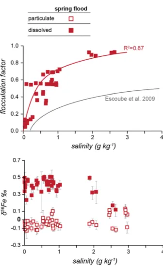
2007; Escoube et al. 2009). These flocculates might sink to the surface sediment or might be transported out of the estuaries (Daneshvar 2015). The amount of Fe flocculating at a certain salinity can be calculated. The flocculation factor F represents the fraction of DFe, which is removed by colloidal flocculation, with 1 equals 100% removal of DFe (Boyle et al. 1974;
Escoube et al. 2009). The flocculation factor is calculated using two system end members, DFe and the salinity (S) of each sample. The samples R1a_05 (16.3 µmol/L DFe) and K1a_05 (17.3 µmol/L) are defined as the river end members, as they have relatively high Fe values and low salinity (< 0.02 g kg−1). The seawater end member should have less than 1% of the initial Fe concentration, we defined sample A13b_05 (0.1 µmol/L; 3 g kg−1), as it showed the highest salinity concentration.
The flocculation factor was calculated for the spring flood estuary data (Fig. 7), about 75% of the DFe flocculated at salinities below 1 g/kg and about 90% at salinities below 3 g/
F=1− (FeSW
FeRW+FeS−FeSW FeRW ∗ 1
1−S∕35 )
kg. In comparison, Escoube et al. (2009) showed removal of DFe by colloidal floccula- tion of 50% below a salinity of 5 g/kg in the North River, which increased to 70% until a salinity of 10 g/kg. At salinities > 10 g/kg, the flocculation is stable between 70 and 80%.
Our values indicate a higher removal of DFe at lower salinities in the estuaries compared to the North River. Earlier studies have suggested major removal of Fe between salini- ties of 5–15 g/kg in the Mullica estuary (USA) and the Amazonas and Para River (Brasil) (Boyle et al. 1974; Sholkovitz et al. 1978). Within boreal estuaries in Finland, significant removal at salinities below 2 g/kg was observed (Asmala et al. 2014). Increasing pH along the estuaries can affect the flocculation and precipitation of Fe oxides and hydroxides. At pH values below 6.5, the oxidation rate normally is low, while at higher pH values [e.g.
7.4–8.6; (Daneshvar 2015)] Fe oxides precipitate as hydrated ferric oxides. In both the Kalix and Råne estuaries, we observed an increase of pH from 6.5 to 7.4 between May and June 2013, which would increase the possibility to form solid-phase ferric iron oxides or hydroxides within the estuaries (Daneshvar 2015). Furthermore, the stability of Fe colloids and particles depends on their composition. The relationship between Fe and OC controls the stability of Fe colloids and aggregates during estuarine mixing and is highly dependent
Fig. 7 Flocculation factor of Fe and δ56Fe versus salinity for Kalix and Råne estuaries during spring flood. The flocculation factor is calculated after Escoube et al. 2009 and for comparison their flocculation trend for the North River, Massachusetts, is displayed in grey in the upper panel. Open symbols display the particulate phase, while filled symbols display the dissolved phase. The error for δ56Fe is presented as 2SD
on the initial Fe:OC ratio (Asmala et al. 2014; Kritzberg et al. 2014; Jilbert et al. 2017).
The aggregates and flocculates are removed from the water column by gravitational set- tling. Small, and therefore light, flocculates might remain suspended in the estuarine waters and travel out to the open sea. Lower total Fe concentrations in the open Bothnian Bay (A5) compared to the estuaries indicate that more Fe is scavenged out between station A5 and the estuaries.
The DFe concentrations in the estuaries during pre- and post-flood are much lower than during spring flood. The only exceptions are the surface waters, which showed elevated DFe concentrations during pre-flood. Studies of DFe and PFe in sea ice showed that the two Fe phases are enriched in the newly built ice (Lannuzel et al. 2010; Janssens et al.
2016). Drilling through the ice and accompanied ice melting might have caused the high DFe and PFe concentrations in the surface waters. Contamination of the water profile by sediment, which got redistributed to the water column, might cause the extreme PFe con- centrations at station R1 during late spring flood.
Within both estuaries, we could observe the same two groups of Fe-isotopes that were observed in their rivers during spring flood (Fig. 7). In our study, DFe has a positive Fe- isotope composition from +0.11 to +0.49‰, within the range of earlier studies, which showed Fe-isotope compositions of various rivers between −1.2 and +1.8‰ (Ilina et al.
2013; Escoube et al. 2015; Zhang et al. 2015; Opfergelt et al. 2017). The PFe phase on the other hand shows lower and mostly negative Fe-isotope values (− 0.13 to 0.09‰) compa- rable to published values in the range of −0.87 to +0.40‰ (Ingri et al. 2006; Ilina et al.
2016; Cheng et al. 2017; Opfergelt et al. 2017). The Fe-isotope signal in both fractions is stable during spring flood, suggesting that the source of the signal is available over a longer period. The particles formed during spring flood in the organic-rich soils are transported along the river through the river mouth into the estuaries. Therefore, in contrast to the Fe concentrations, the Fe-isotope compositions are stable along the salinity gradient. Within the Bothnian Bay, PFe-isotope values are slightly heavier than in the estuaries. We could not detect the negative Fe-isotope signal in the Bothnian Bay. Hence, the negative par- ticles might be removed from the water column during estuarine mixing. The driver for the removal could be the different surface properties of the Fe-OC and Fe(oxy)hydroxide aggregates, which lead to different flocculation behaviours along the estuaries (Gustafsson et al. 2000).
Particulate Fe-isotope values during pre- and post-flood in the rivers, estuaries and the Bothnian Bay are generally heavier compared to values during spring flood. During pre- flood, the estuaries show values around +0.2‰, while during post-flood, the measured val- ues are higher around +0.4‰. Suggesting that PFe delivers positive Fe-isotope values dur- ing base flow conditions in contrast to the spring flood. The post-flood PFe-isotope values in the Bothnian Bay are as high as +0.6‰ exceeding values found during earlier research [+0.1 to +0.2‰, (Gelting 2009)].
6 Conclusions
First of all, this study shows the stability of a natural system over decades. Earlier research in the Kalix River [since 1982, e.g. (Pontér et al. 1990; Ingri 1996)] showed similar behav- iour of the Fe concentration and Fe-isotopes. The annual spring flood with the accompany- ing features of increasing Fe concentrations and decreasing Fe-isotope compositions is a regular and periodic event influencing the water geochemistry. Our data set complements