Seasonal prediction of equatorial Atlantic sea surface temperature using simple initialisation and bias correction techniques — Supporting Information —

Seasonal prediction of equatorial Atlantic sea surface temperature using simple initialisation and bias

correction techniques

— Supporting Information —

Tina Dippe

, Richard J. Greatbatch

, and Hui Ding

1

GEOMAR Helmholtz Centre for Ocean Research Kiel, Germany

2

Faculty of Mathematics and Natural Sciences, Christian Albrechts Universit¨ at, Kiel, Germany

3

Cooperate Institute for Research in Environmental Sciences - University of Colorado and NOAA Earth Systems Research Laboratory,

Boulder, USA

November 15, 2018

1 Bias Correction and Skill of Initial Conditions in the Equatorial Pacific

As for the equatorial Atlantic, heat flux correction improves the mean state and the simulated variability in the KCM’s equatorial Pacific (Figs. S1 and S2). The NINO3.4-region ( [-5 5]^◦N, [-170 -120]^◦E) in the KCM suffers from a cold bias (Fig.

S1) with a magnitude of 0.93 (1.21) and 1.17 (0.98)^◦C in FLX (STD) for the annual mean and September-December, respectively. Heat flux correction does not reduce the SST bias in Nino3.4 in boreal fall. It seems that in boreal fall in the equatorial Pacific, whatever is causing the cold SST bias is too strong to be ameliorated by our simple surface flux correction. The result is that FLX is hardly distinguishable from STD in boreal fall. In boreal spring and summer on the other hand (March- July), when the cold bias in the eastern cold tongue region is strongest (1.53^◦C), FLX reduces the bias to 0.80^◦.

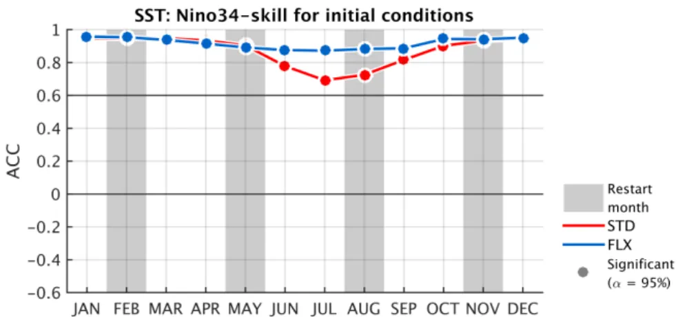
Initial conditions for SST are generally good in the tropical Pacific for the dynam- ical hindcasts (Fig. S2). ACCs between the initialisation runs and ERA-Interim are 0.92 (0.87) on average and minimum during July (July) with a value of 0.87 (0.69) in the FLX (STD) initialisation run. Note that heat flux correction improves the ability of the KCM to simulate interannual variability in boreal summer, particularly in July and August. This is interesting, because the SST bias during these months is comparable in both initialisation runs.

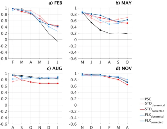
The predictive skill of the hindcasts for SST in the NINO3.4-region is shown in Fig. S3. Generally speaking, there are no consistent differences between STD and FLX hindcasts. Predictive skill shows a marked seasonality. The hindcasts lose skill relatively quickly for forecasts that are initialized in February and to some extent in May, although they generally do better than persistence, especially when initialised in May. In contrast, hindcasts that are started during August and November retain high skill until the end of the hindcasting period, although not better than persistence.

November hindcast skill is the best.

Note that the simple initialisation technique of partial coupling in the KCM pro- duces initial conditions that sustain rather successful hindcasts for the tropical Pacific.

Indeed, the skill of our NINO3.4 hindcasts is comparable to the skill of other seasonal forecasting systems (e.g.Baehr et al., 2014).

1

References

Baehr, J., K. Fr¨ohlich, M. Botzet, D. I. V. Domeisen, L. Kornblueh, D. Notz, R. Pio- ntek, H. Pohlmann, S. Tietsche, and W. A. M¨uller (2014), The prediction of surface temperature in the new seasonal prediction system based on the MPI-ESM coupled climate model,Climate Dynamics, pp. 1–13, doi:10.1007/s00382-014-2399-7.

2 List of supplementary Figures

Figure S1: Monthly mean SST in (black) ERA-Interim and the (blue) FLX and (red) STD initialisation runs, area-averaged over the NINO3.4 Region: [-5,5]^◦N, [- 170,-120]^◦E

3

Figure S2: Monthly anomaly correlation coefficient between ERA-Interim and the KCM initialisation runs for the (blue) FLX and (red) STD experiments in the NINO3.4-region. ACC-values that are significantly different from 0 at the 95%-level are shown as circles. Grey background bars show months during which seasonal hind- casts have been started from the initialisation runs.

Figure S3: Skill (ACC) for SST in NINO3.4 for hindcasts started at the beginning of (a) February, (b) May, (c) August, (d) November. Circles show ACCs that are significantly different from 0 at the 95%-level. Line colours show the different exper- iments (see main text for details): (black) reference persistence forecast, (light red) dynamical STD, (light blue) dynamical FLX, (red) corrected STD, (blue) corrected FLX.

5

Figure S4: Same as Figure S1 but for zonal wind stress in the WAtl region ([-3,3]^◦N, [-40,-20]^◦E).