Edwin L. Woollett October 21, 2010
Contents
6 Differential Calculus 3
6.1 Differentiation of Explicit Functions . . . . 4
6.1.1 All Aboutdiff . . . . 4
6.1.2 The Total Differential . . . . 5
6.1.3 Controlling the Form of a Derivative withgradef . . . . 6
6.2 Critical and Inflection Points of a Curve Defined by an Explicit Function . . . . 7
6.2.1 Example 1: A Polynomial . . . . 7
6.2.2 Automating Derivative Plots withplotderiv . . . . 9
6.2.3 Example 2: Another Polynomial . . . . 11
6.2.4 Example 3: x2/3, Singular Derivative, Use oflimit . . . . 12
6.3 Tangent and Normal of a Point of a Curve Defined by an Explicit Function . . . . 13
6.3.1 Example 1: x2 . . . . 14
6.3.2 Example 2: ln(x) . . . . 14
6.4 Maxima and Minima of a Function of Two Variables . . . . 15
6.4.1 Example 1: Minimize the Area of a Rectangular Box of Fixed Volume . . . . 16
6.4.2 Example 2: Maximize the Cross Sectional Area of a Trough . . . . 18
6.5 Tangent and Normal of a Point of a Curve Defined by an Implicit Function . . . . 19
6.5.1 Tangent of a Point of a Curve Defined byf(x,y) =0 . . . . 21
6.5.2 Example 1: Tangent and Normal of a Point of a Circle . . . . 23
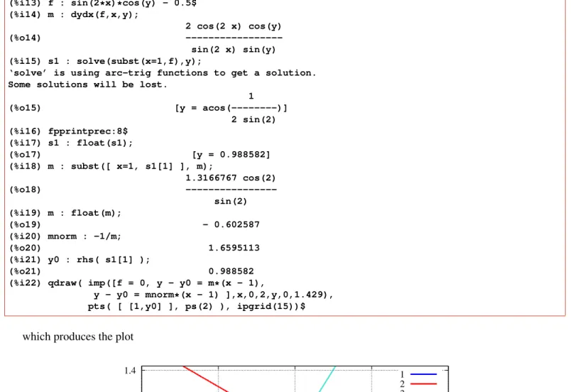
6.5.3 Example 2: Tangent and Normal of a Point of the Curvesin(2x) cos(y) = 0.5 . . . . 25
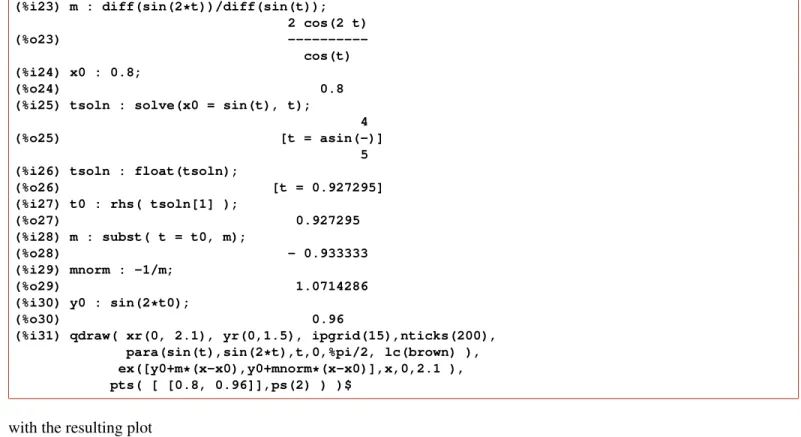
6.5.4 Example 3: Tangent and Normal of a Point on a Parametric Curve:x=sin(t),y=sin(2 t) . . . . 26
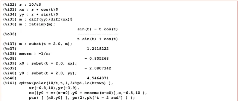
6.5.5 Example 4: Tangent and Normal of a Point on a Polar Plot:x=r(t)cos(t),y=r(t)sin(t) . . . . 27
6.6 Limit Examples Using Maxima’slimitFunction . . . . 28
6.6.1 Discontinuous Functions . . . . 29
6.6.2 Indefinite Limits . . . . 32
6.7 Taylor Series Expansions usingtaylor . . . . 34
6.8 Vector Calculus Calculations and Derivations usingvcalc.mac . . . . 36
6.9 Maxima Derivation of Vector Calculus Formulas inCylindrical Coordinates . . . . 40
6.9.1 The Calculus Chain Rule in Maxima . . . . 41
6.9.2 Laplacian ∇2f(ρ, ϕ, z) . . . . 43
6.9.3 Gradient ∇f(ρ, ϕ, z) . . . . 45
6.9.4 Divergence ∇ ·B(ρ, ϕ, z) . . . . 48
6.9.5 Curl ∇ ×B(ρ, ϕ, z) . . . . 49
6.10 Maxima Derivation of Vector Calculus Formulas inSpherical Polar Coordinates . . . . 50
∗This version uses Maxima 5.21.1 This is a live document. Check http://www.csulb.edu/˜woollett/ for the latest version of these notes. Send comments and suggestions towoollett@charter.net
1
This document is part of a series of notes titled
"Maxima by Example" and is made available
via the author’s webpage http://www.csulb.edu/˜woollett/
to aid new users of the Maxima computer algebra system.
NON-PROFIT PRINTING AND DISTRIBUTION IS PERMITTED.
You may make copies of this document and distribute them
to others as long as you charge no more than the costs of printing.
These notes (with some modifications) will be published in book form eventually via Lulu.com in an arrangement which will continue
to allow unlimited free download of the pdf files as well as the option of ordering a low cost paperbound version of these notes.
Feedback from readers is the best way for this series of notes to become more helpful to new users of Maxima. All comments and suggestions for improvements will be appreciated and carefully considered.
LOADING FILES
The defaults allow you to use the brief version load(fft) to load in the Maxima file fft.lisp.
To load in your own file, such as qxxx.mac
using the brief version load(qxxx), you either need to place qxxx.mac in one of the folders Maxima searches by default, or else put a line like:
file_search_maxima : append(["c:/work2/###.{mac,mc}"],file_search_maxima )$
in your personal startup file maxima-init.mac (see later in this chapter for more information about this).
Otherwise you need to provide a complete path in double quotes, as in load("c:/work2/qxxx.mac"),
We always use the brief load version in our examples, which are generated using the XMaxima graphics interface on a Windows XP computer, and copied into a fancy verbatim environment in a latex file which uses the fancyvrb and color packages.
Maxima.sourceforge.net. Maxima, a Computer Algebra System. Version 5.21.1 (2010). http://maxima.sourceforge.net/
The homemade functionfll(x)(first, last, length) is used to return the first and last elements of lists (as well as the length), and is automatically loaded in withmbe1util.macfrom Ch. 1. We will include a reference to this definition when working with lists.
This function has the definitions
fll(x) := [first(x),last(x),length(x)]$
declare(fll,evfun)$
Some of the examples used in these notes are from the Maxima html help manual or the Maxima mailing list:
http://maxima.sourceforge.net/maximalist.html.
The author would like to thank the Maxima developers for their friendly help via the Maxima mailing list.
2
6 Differential Calculus
The methods of calculus lie at the heart of the physical sciences and engineering.
The student of calculus needs to take charge of his or her own understanding, taking the subject apart and putting it back together again in a way that makes logical sense. The best way to learn any subject is to work through a large collection of problems. The more problems you work on your own, the more you “own” the subject. Maxima can help you make faster progress, if you are just learning calculus.
For those who are already calculus savvy, the examples in this chapter will offer an opportunity to see some Maxima tools in the context of very simple examples, but you will likely be thinking about much harder problems you want to solve as you see these tools used here.
After examples of usingdiff andgradef, we present examples of finding the critical and inflection points of plane curves defined by an explicit function.
We then present examples of calculating and plotting the tangent and normal to a point on a curve, first for explicit func- tions and then for implicit functions.
We also have two examples of finding the maximum or minimum of a function of two variables.
We then present several examples of using Maxima’s powerfullimitfunction, followed by several examples of using taylor.
The next section shows examples of using the vector calculus functions (as well as cross product) in the package vcalc.mac, developed by the author and available on his webpage with this chapter, to calculate the gradient, di- vergence, curl, and Laplacian in cartesian, cylindrical, and spherical polar coordinate systems. An example of using this package would becurl([r*cos(theta),0,0]);(if the current coordinate system has already been changed to spherical polar) orcurl([r*cos(theta),0,0], s(r,theta,phi) ); if the coordinate system needs to be shifted to spherical polar from either cartesian (the starting default) or cylindrical.
The order of list vector components corresponds to the order of the arguments ins(r,theta,phi). The Maxima output is the list of the vector curl components in the current coordinate system, in this case[0, 0, sin(theta)]
plus a reminder to the user of what the current coordinate system is and what symbols are currently being used for the independent variables.
Thus the syntax is based on lists and is similar (although better!) than Mathematica’s syntax.
There is a separate function to change the current coordinate system. To set the use of cylindrical coordinates(rho,phi,z):
setcoord( cy(rho,phi,z) );
and to set cylindrical coordinates(r,t,z):
setcoord( cy(r,t,z) );
The packagevcalc.macalso contains the plotting functionplotderivwhich is useful for “automating” the plotting of a function and its firstnderivatives.
The next two sections dicuss the use of the batch file mode of problem solving by presenting Maxima based derivations of the form of the gradient, divergence, curl, and Laplacian by starting with the cartesian forms and changing variables to (separately) cylindrical and spherical polar coordinates. (The batch files used arecylinder.macandsphere.mac.) These two sections show Maxima’s implementation of the calculus chain rule at work with use of bothdependsand gradef.
6.1 Differentiation of Explicit Functions
We begin with explicit functions of a single variable. After giving a few examples of the use of Maxima’sdifffunction, we will discuss critical and inflection points of curves defined by explicit functions, and the construction and plotting of the tangent and normal of a point of such curves.
6.1.1 All About diff
The commanddiff(expr,var,num)will differentiate the expresssion in slot one with respect to the variable entered in slot two a number of times determined by a positive integer in slot three. Unless a dependency has been established, all parameters and “variables” in the expression are treated as constants when taking the derivative.
Thusdiff(expr,x,2)will yield the second derivative ofexprwith respect to the variablex.
The simple formdiff(expr, var)is equivalent todiff(expr,var,1).
If the expression depends on more than one variable, we can use commands such asdiff(expr,x,2,y,1)to find the result of taking the second derivative with respect tox(holdingyfixed) followed by the first derivative with respect toy(holdingxfixed).
Here are some simple examples.
We first calculate the derivative ofxn.
(%i1) diff(xˆn,x);
n - 1
(%o1) n x
Next we calculate the third derivative ofxn.
(%i2) diff(xˆn,x,3);
n - 3
(%o2) (n - 2) (n - 1) n x
Here we take the derivative (with respect to x) of an expression depending on bothxandy.
(%i3) diff(xˆ2 + yˆ2,x);
(%o3) 2 x
You can differentiate with respect to any expression that does not involve explicit mathematical operations.
(%i4) diff( x[1]ˆ2 + x[2]ˆ2, x[1] );
(%o4) 2 x
1
Note thatx1 is Maxima’s way of “pretty printing”x[1]. We can use thegrindfunction to display the output%o4in the “non-pretty print mode” (what would have been returned if we had set thedisplay2dswitch tofalse).
(%i5) grind(%)$
2*x[1]$
(%i6) display2d$
Note the dollar signgrindadds to the end of its output.
Finally, an example of using one invocation ofdiffto differentiate with respect to more than one variable:
(%i7) diff(xˆ2*yˆ3,x,1,y,2);
(%o7) 12 x y
6.1.2 The Total Differential
If you use thediff function without a symbol in slot two, Maxima returns the “total differential” of the expression in slot one, and by default assumes every parameter is a variable.
If an expression contains a single parameter, sayx, thendiff(expr)will generate
d f (x) =
µ d f (x) d x
d x (6.1)
In the first example below, we calculate the differential of the expressionx2, that is, the derivative of the expression (with respect to the variablex) multiplied by “the differential of the independent variablex”,d x. Maxima usesdel(x)for the differential ofx, a small increment ofx.
(%i1) diff(xˆ2);
(%o1) 2 x del(x)
If the expression contains two parametersxandy, then the total differential is equivalent to the Maxima expression diff(expr,x)*del(x) + diff(expr,y)*del(y) ,
which generates (using conventional notation):
d f (x, y) =
µ ∂f (x, y)
∂x
y
d x +
µ ∂f (x, y)
∂y
x
d y. (6.2)
Each additional parameter induces an additional term of the same form.
(%i2) diff(xˆ2*yˆ3);
2 2 3
(%o2) 3 x y del(y) + 2 x y del(x)
(%i3) diff(a*xˆ2*yˆ3);
2 2 3 2 3
(%o3) 3 a x y del(y) + 2 a x y del(x) + x y del(a)
We can use thesubstfunction to replace, saydel(x), by anything else:
(%i4) subst(del(x) = dx, %o1);
(%o4) 2 dx x
(%i5) subst([del(x)= dx, del(y) = dy, del(a) = da],%o3 );
2 3 3 2 2
(%o5) da x y + 2 a dx x y + 3 a dy x y
You can use thedeclarefunction to prevent some of the symbols from being treated as variables when calculating the total differential:
(%i6) declare (a, constant)$
(%i7) diff(a*xˆ2*yˆ3);
2 2 3
(%o7) 3 a x y del(y) + 2 a x y del(x) (%i8) declare([b,c],constant)$
(%i9) diff( a*xˆ3 + b*xˆ2 + c*x );
2
(%o9) (3 a x + 2 b x + c) del(x)
(%i10) properties(a);
(%o10) [database info, kind(a, constant)]
(%i11) propvars(constant);
(%o11) [a, b, c]
(%i12) kill(a,b,c)$
(%i13) propvars(constant);
(%o13) []
(%i14) diff(a*x);
(%o14) a del(x) + x del(a)
We can “map”diffon to a list of functions ofx, say, and divide bydel(x), to generate a list of derivatives, as in
(%i15) map(’diff,[sin(x),cos(x),tan(x) ] )/del(x);
2
(%o15) [cos(x), - sin(x), sec (x)]
(%i16) map(’diff,%)/del(x);
2
(%o16) [- sin(x), - cos(x), 2 sec (x) tan(x)]
6.1.3 Controlling the Form of a Derivative with gradef
We can usegradefto select one from among a number of alternative ways of writing the result of differentiation. The large number of “trigonometric identities” means that any given expression containing trig functions can be written in terms of a different set of trig functions.
As an example, consider trig identities which expresssin(x),cos(x), andsec2(x)in terms oftan(x)andtan(x/2):
sec
2(x) = 1 + tan
2(x), (6.3)
sin x = 2 tan(x/2)/(1 + tan
2(x/2)), (6.4) cos x = (1 − tan
2(x/2))/(1 + tan
2(x/2)). (6.5)
The default Maxima result for the first derivatives ofsinx,cosx, andtanxis:
(%i1) map(’diff,[sin(x),cos(x),tan(x)] )/del(x);
2
(%o1) [cos(x), - sin(x), sec (x)]
Before usinggradefto alter the return value ofdifffor these three functions, let’s check that Maxima agrees with the trig “identities” displayed above. Variable amounts of expression simplification are needed to get what we want.
(%i2) trigsimp( 1 + tan(x)ˆ2 );
1
(%o2) ---
2 cos (x)
(%i3) ( trigsimp( 2*tan(x/2)/(1 + tan(x/2)ˆ2) ), trigreduce(%%) );
(%o3) sin(x)
(%i4) ( trigsimp( (1-tan(x/2)ˆ2)/(1 + tan(x/2)ˆ2) ), trigreduce(%%), expand(%%) );
(%o4) cos(x)
Recall thattrigsimpwill converttan,sec, etc tosinandcosof the same argument. Recall also thattrigreduce will convert an expression containingcos(x/2)andsin(x/2)into an expression containingcos(x)andsin(x).
Finally, remembering thatsecx= 1/cosx, we see that Maxima has “passed the test”.
Now let’s usegradefto express the derivatives in terms oftanxandtan(x/2):
(%i5) gradef(tan(x), 1 + tan(x)ˆ2 );
(%o5) tan(x)
(%i6) gradef(sin(x),(1-tan(x/2)ˆ2 )/(1 + tan(x/2)ˆ2 ) );
(%o6) sin(x)
(%i7) gradef(cos(x), -2*tan(x/2)/(1 + tan(x/2)ˆ2 ) );
(%o7) cos(x)
Here we check the behavior:
(%i8) map(’diff,[sin(x),cos(x),tan(x)] )/del(x);
2 x x
1 - tan (-) 2 tan(-)
2 2 2
(%o8) [---, - ---, tan (x) + 1]
2 x 2 x
tan (-) + 1 tan (-) + 1
2 2
6.2 Critical and Inflection Points of a Curve Defined by an Explicit Function
Thecritical pointsof a functionf(x)are the pointsxjsuch thatf0(xj) =0. We will usef0to indicate the first derivative, andf00 to indicate the second derivative. The extrema (ie., maxima and minima) are the values of the function at the critical points, provided the “slope”f0 actually has a different sign on the opposite sides of the critical point.
Maximum:f0(a) =0, f0(x) changes from+to− , f00(a)<0 Minimum:f0(a) =0, f0(x) changes from−to+ , f00(a)>0
Iff(x)is a function with a continuous second derivative, and if, asxincreases through the valuea,f00(x)changes sign, then the plot off(x)has aninflection pointatx=aandf00(a) =0. Theinflection pointrequirement thatf00(x)changes sign atx=ais equivalent tof000(a)6=0. We consider some simple examples taken from Sect. 126 of Analytic Geometry and Calculus, by Lloyd L. Smail, Appleton-Century-Crofts, N.Y., 1953 (a reference which “dates” the writer of these notes!).
6.2.1 Example 1: A Polynomial
To find the maxima and minima of the functionf(x) =2 x3−3 x2−12 x+13, we use an “expression” (called g) rather than a Maxima function. We usegp(g prime) for the first derivative, andgpp(g double prime) as notation for the second derivative. Since we will want to make some simple plots, we use the packageqdraw, available on the author’s webpage, and discussed in detail in chapter five of these notes.
(%i1) load(draw)$
(%i2) load(qdraw);
qdraw(...), qdensity(...), syntax: type qdraw();
(%o2) c:/work2/qdraw.mac
(%i3) g : 2*xˆ3 - 3*xˆ2 - 12*x + 13$
(%i4) gf : factor(g);
2
(%o4) (x - 1) (2 x - x - 13)
(%i5) gp : diff(g,x);
2
(%o5) 6 x - 6 x - 12
(%i6) gpf : factor(gp);
(%o6) 6 (x - 2) (x + 1)
(%i7) gpp : diff(gp,x);
(%o7) 12 x - 6
(%i8) qdraw( ex(g,x,-4,4), key(bottom) )$
Since the coefficients of the given polynomial are integral, we have tried outfactoron both the given expression and its first derivative. We see from output%o6 that the first derivative vanishes whenx = -1, 2 . We can confirm these critical points of the given function by usingqdrawwith the quick plotting argumentex, which gives us the plot:
-100 -80 -60 -40 -20 0 20 40
-4 -3 -2 -1 0 1 2 3 4
1
Figure 1: Plot of g over the range[−4,4]
We can use the cursor on the plot to find thatgtakes on the value of roughly-7whenx = 2and the value of about 20whenx = -1. We can usesolveto find the roots of the equationgp = 0, and then evaluate the given expression g, as well as the second derivativegppat the critical points found:
(%i9) solve(gp=0);
(%o9) [x = 2, x = - 1]
(%i10) [g,gpp],x=-1;
(%o10) [20, - 18]
(%i11) [g,gpp],x=2;
(%o11) [- 7, 18]
We next look for theinflection points, the points where the curvature changes sign, which is equivalent to the points where the second derivative vanishes.
(%i12) solve(gpp=0);
1
(%o12) [x = -]
2 (%i13) g,x=0.5;
(%o13) 6.5
We have found one inflection point, that is a point on a smooth curve where the curve changes from concave downward to concave upward, or visa versa (in this case the former).
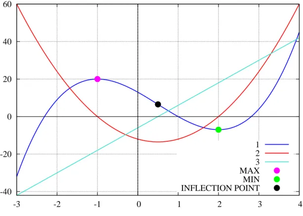
We next plotg, gp, gpptogether.
(%i14) qdraw2( ex([g,gp,gpp],x,-3,3), key(bottom),
pts([[-1,20]],ps(2),pc(magenta),pk("MAX") ), pts([[2,-7]],ps(2),pc(green),pk("MIN") ),
pts([[0.5, 6.5]],ps(2),pk("INFLECTION POINT") ) )$
with the resulting plot:
-40 -20 0 20 40 60
-3 -2 -1 0 1 2 3 4
1 2 3 MAX MIN INFLECTION POINT
Figure 2: Plot of 1: g, 2: gp, and 3: gpp
The curvegis concave downward untilx = 0.5and then is concave upward. Note that each successive differentia- tion tends to flatten out the kinks in the previous expression (function). In other words,gpis “flatter” thang, andgppis
“flatter” thangp. This behavior underdiffis simply because each successive differentiation reduces by one the degree of the polynomial.
6.2.2 Automating Derivative Plots with plotderiv
In a separate text file vcalc.mac(available on the author’s webpage) is a small homemade Maxima function called plotderivwhich will plot a given expression together with as many derivatives as you want, usingqdrawfrom Ch.5.
/* vcalc.mac */
plotderiv_syntax() :=
disp("plotderiv(expr,x,x1,x2,y1,y2,numderiv) constructs a list of the submitted expression expr and its first numderiv derivatives with respect to the independent variable, and then passes
this list to qdraw(..). You need to have used load(draw) and load(qdraw) before using this function ")$
/* version 1 commented out
plotderiv(expr,x,x1,x2,y1,y2,numderiv) :=
block([plist], plist : [],
for i thru numderiv do
plist : cons(diff(expr,x,i), plist), plist : reverse(plist),
plist : cons(expr, plist), display(plist),
apply( ’qdraw, [ ex( plist,x,x1,x2 ),yr(y1,y2), key(bottom) ]))$ */
/* version 2 slightly more efficient */
plotderiv(expr,x,x1,x2,y1,y2,numderiv) :=
block([plist,aa], plist : [], aa[0] : expr,
for i thru numderiv do ( aa[i] : diff(aa[i-1],x), plist : cons(aa[i], plist)
),
plist : reverse(plist), plist : cons(expr, plist), display(plist),
apply( ’qdraw, [ ex( plist,x,x1,x2 ),yr(y1,y2), key(bottom) ]))$
We have provided two versions of this function, the first version commented out. If the expression to be plotted is a very complicated function and you are concerned with computing time, you can somewhat improve the efficiency of plotderivby introducing a “hashed array” calledaa[j], say, to be able to simply differentiate the previous deriva- tive expression. That is the point of version 2 which is not commented out.
We have added the linedisplay(plist) to print a list containing the expression as well as all the derivatives re- quested. We testplotderivon the expressionuˆ3. Bothdraw.lisp andqdraw.macmust be loaded for this to work.
(%i15) load(vcalc)$
vcalc.mac: for syntax, type: vcalc_syntax();
CAUTION: global variables set and used in this package:
hhh1, hhh2, hhh3, uuu1, uuu2, uuu3, nnnsys (%i16) plotderiv(uˆ3,u,-3,3,-27,27,4)$
3 2
plist = [u , 3 u , 6 u, 6, 0]
which produces the plot:
-20 -10 0 10 20
-3 -2 -1 0 1 2 3
1 2 3 4 5
Figure 3: 1: u3, 2: 3 u2, 3:6 u, 4:6, 5:0
6.2.3 Example 2: Another Polynomial
We find the critical points, inflection points, and extrema of the expression3 x4−4 x3. We first look at the expression and its first two derivatives usingplotderiv.
(%i17) plotderiv(3*xˆ4 - 4*xˆ3,x,-1,3,-5,5,2)$
4 3 3 2 2
plist = [3 x - 4 x , 12 x - 12 x , 36 x - 24 x]
which produces the plot:
-4 -2 0 2 4
-1 -0.5 0 0.5 1 1.5 2 2.5 3
1 2 3
Figure 4: 1:f =3 x4−4 x3, 2: f0, 3: f00
We have inflection points atx=0, 2/3since the second derivative is zero at both points and changes sign as we follow the curve through those points. The curve changes from concave up to concave down passing throughx=0, and changes from concave down to concave up passing throughx=2/3. The following provides confirmation of our inferences from the plot:
(%i18) g:3*xˆ4 - 4*xˆ3$
(%i19) g1: diff(g,x)$
(%i20) g2 : diff(g,x,2)$
(%i21) g3 : diff(g,x,3)$
(%i22) x1 : solve(g1=0);
(%o22) [x = 0, x = 1]
(%i23) gcrit : makelist(subst(x1[i],g),i,1,2);
(%o23) [0, - 1]
(%i24) x2 : solve(g2=0);
2
(%o24) [x = -, x = 0]
3
(%i25) ginflec : makelist( subst(x2[i],g ),i,1,2 );
16
(%o25) [- --, 0]
27
(%i26) g3inflec : makelist( subst(x2[i],g3),i,1,2 );
(%o26) [24, - 24]
We have critical points where the first derivative vanishes atx=0, 1. Since the first derivative does not change sign as the curve passes through the pointx=0, that point is neither a maximum nor a mimimum point. The pointx=1is a minimum point since the first derivative changes sign from negative to positive as the curve passes through that point.
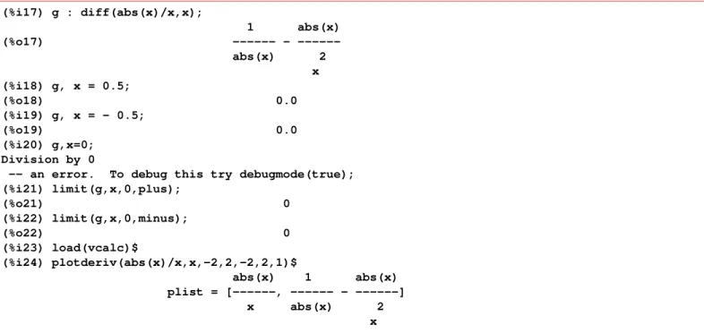
6.2.4 Example 3:x2/3, Singular Derivative, Use of limit
Searching for points where a function has a minimum or maximum by looking at points where the first derivative is zero is useful as long as the first derivative is well behaved. Here is an example in which the given function ofxhas a minimum atx=0, but the first derivative is singular at that point. Using the expressiong = xˆ(2/3)withplotderiv:
(%i27) plotderiv(xˆ(2/3),x,-2,2,-2,2,1)$
-2 -1.5 -1 -0.5 0 0.5 1 1.5 2
-2 -1.5 -1 -0.5 0 0.5 1 1.5 2
1 2
Figure 5: Plot of1: f(x) =x2/3, 2: f0
We see that the first derivative is singular atx=0and approaches either positive or negative infinity, depending on your direction of approaching the pointx=0. We can see from the plot off(x) =x2/3that the tangent line (the “slope”) of the curve is negative forx<0and becomes increasingly negative (approaching minus infinity) as we approach the point x=0from the negative side. We also see from the plot off(x) that the tangent line (“slope”) is positive for positive values ofxand as we passx=0, moving from smallerxto largerxthat the sign of the first derivativef0(x) changes from−to+, which is a signal of a local minimum of a function.
We can practice using the Maxima functionlimitwith this example:
(%i28) gp : diff(xˆ(2/3),x);
2
(%o28) ---
1/3 3 x (%i29) limit(gp,x,0,plus);
(%o29) inf
(%i30) limit(gp,x,0,minus);
(%o30) minf
(%i31) limit(gp,x,0);
(%o31) und
The most frequent use of the Maximalimitfunction has the syntax Function:limit (expr, x, val, dir)
Function:limit (expr, x, val)
The first form computes the limit ofexpras the real variablexapproaches the valuevalfrom the direction dir.dirmay have the valueplusfor a limit from above,minusfor a limit from below.
In the second form,diris omitted, implying a “two-sided limit” is to be computed.
limituses the following special symbols: inf(positive infinity) andminf(negative infinity). On output it may also useund(undefined),ind(indefinite but bounded) andinfinity(complex infinity).
Returning to our example, if we ignore the pointx=0, the slope is always decreasing, so the second derivative is always negative.
6.3 Tangent and Normal of a Point of a Curve Defined by an Explicit Function
The equation of a line with the formy=m(x−x0) +y0, wherem,x0, andy0are constants, is identically satisfied if we consider the point(x,y) = (x0,y0). Hence this line passes through the point(x0,y0). The “slope” of this line (the first derivative) is the constantm.
Now we also assume that the point(x0,y0) is a point of a curve given by some explicit function ofx, sayy=f(x);
hencey0=f(x0). The first derivative of this function, evaluated at the pointx0 is the local “slope”, which defines the local tangent line, y=m(x−x0) +y0, if we use formthe value off0(x0), where the notation means first take the derivative for arbitraryxand then evaluate the derivative atx=x0.
Let the two dimensional vectortvecbe a vector parallel to the tangent line (at the point of interest) with components (tx,ty), such that the vector makes an angleθwith the positivexaxis. Thentan(θ)=ty/tx=m=d y/d xis the slope of the tangent (line) at this point. Let the two dimensional vectornvecwith components(nx,ny)be parallel to the lineperpendicularto the tangent at the given point. Thisnormalline will be perpendicular to the tangent line if the vectorsnvecandtvecare perpendicular (i.e., “orthogonal”).
In Maxima, we can represent vectors by lists:
(%i1) tvec : [tx,ty];
(%o1) [tx, ty]
(%i2) nvec : [nx, ny];
(%o2) [nx, ny]
Two vectors are “orthogonal” if the “dot product” is zero. A simple example will illustrate this general property. Consider the pair of unit vectors:ivec = [1,0], parallel to the positivexaxis andjvec = [0,1], parallel to the positivey axis.
(%i3) ivec : [1,0]$
(%i4) jvec : [0,1]$
(%i5) ivec . jvec;
(%o5) 0
Since Maxima allows us to use aperiodto find the dot product (inner product) of two lists (two vectors), we will ensure that the normal vector is “at right angles” to the tangent vector by requiringnvec . tvec = 0
(%i6) eqn : nvec . tvec = 0;
(%o6) ny ty + nx tx = 0
(%i7) eqn : ( eqn/(nx*ty), expand(%%) );
tx ny
(%o7) -- + -- = 0
ty nx
We represent the normal (the line perpendicular to the tangent line) at the point (x0,y0) asy=mn(x−x0) +y0, wheremnis the slope of the normal line:mn = ny/nx = - (1/(ty/tx)) = -1/m .
In words,the slope of the normal line is the negative reciprocal of the slope of the tangent line.
Thus the equation of thelocal normal to the curve at the point (x0,y0) can be written asy=−(x−x0)/m+y0, wheremis the slope of the local tangent.
6.3.1 Example 1:x2
As an easy first example, let’s use the functionf(x) =x2 and construct the tangent line and normal line to this plane curve at the pointx = 1, y = f(1) = 1. (We have discussed this same example in Ch. 5). The first derivative is 2 x, and its value atx=1is2. Thus the equation of the local tangent to the curve at(x,y) = (1,1)isy=2 x−1.
The equation of the local normal at the same point isy=−x/2+3/2.
We will plot the curvey=x2, the local tangent, and the local normal together. Special care is needed to get the horizontal
“canvas” width about1.4times the vertical height to achieve a geometrically correct plot; otherwise the “normal” line would not cross the tangent line at right angles.
(%i8) qdraw( ex([xˆ2,2*x-1,-x/2+3/2],x,-1.4,2.8), yr(-1,2) , pts( [ [1,1]],ps(2) ) )$
The plot looks like:
-1 -0.5 0 0.5 1 1.5 2
-1 -0.5 0 0.5 1 1.5 2 2.5
1 2 3
Figure 6: Tangent and Normal tox2 at point(1,1)
We can see directly from the plot that the slope of the tangent line has the value2. Remember that we can think of
“slope” as being the number derived from dividing the “rise” by the “run”. Thus if we choose a “run” to be thexinterval (0,1), from the plot this corresponds to the “rise” of1−(−1) =2. Hence “rise/run” is2.
6.3.2 Example 2:ln(x)
Our next example repeats the analysis of Example 1 for the functionln(x), using the point(x=2,y=ln(2)). Maxima’s natural log function is writtenlog. Maxima does not have a “log to the base 10 function”, although you can “roll your own” with a definition likelog10(x) := log(x)/log(10), which is equivalent to log(x)/2.303. Thus in Maxima, log(10) = 2.303, log(2) = 0.693, etc. We are constructing the local tangent and normal at the point(x=2,y=0.693). The derivative of the natural log is
(%i9) diff(log(x),x);
1
(%o9) -
x
so the “slope” of our curve (and the tangent) at the chosen point is 1/2, and the slope of the local normal is -2.
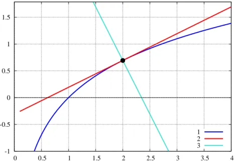
The equation of the tangent is then (y−ln(2)) = (1/2) (x−2), or y=x/2−0.307. The equation of the normal
is(y−ln(2)) =−2(x−2), ory=−2 x+4.693. In order to get a decent plot, we need to stay away from the sin- gular pointx=0, so we start the plot withxa small positive number. We choose to use the x-axis range(0.1,4), then
∆x=3.9. Since we want the “canvas width”∆x≈1.4 ∆y, we need∆y=2.786, which is satisfied if we choose the y-axis range to be(−1,1.786).
(%i10) qdraw(key(bottom), yr(-1,1.786),
ex([log(x), x/2 - 0.307, -2*x + 4.693],x,0.1,4), pts( [ [2,0.693]],ps(2) ) );
which produces the plot:
-1 -0.5 0 0.5 1 1.5
0 0.5 1 1.5 2 2.5 3 3.5 4
1 2 3
Figure 7: Tangent and Normal toln(x)at point(2,ln(2))
6.4 Maxima and Minima of a Function of Two Variables You can find proofs of the following criteria in calculus texts.
Iff(x,y)and its first derivatives are continuous in a region including the point(a,b), a necessary condition thatf(a,b) shall be an extreme (maximum or minimum) value of the functionf(x,y)is that (I):
∂f(a, b)
∂x = 0, ∂f(a, b)
∂y = 0 (6.6)
in which the notation means first take the partial derivatives for arbitraryxandyand then evaluate the resulting deriva- tives at the point(x,y) = (a,b).
Examples show that these two conditions (I) do not guarantee that the function actually takes on an extreme value at the point(a,b), although in many practical problems the existence and nature of an extreme value is often evident from the problem itself and no extra test is needed; all that is needed is thelocationof the extreme value.
If condition (I) is satisfied and if, in addition, at the point(a,b)we have (II):
∆ = µ∂2f
∂ x2
¶ µ∂2f
∂ y2
−
µ ∂2f
∂x ∂y
¶2
> 0 (6.7)
thenf(x,y)will have a maximum value or a minimum value given byf(a,b)according as∂2f /∂ x2
( or∂2f /∂ y2) is negative or positive forx=a,y=b. If condition (I) holds and∆<0thenf(a,b)is neither a maximum nor a minimum; if∆ = 0the test fails to give any information.
6.4.1 Example 1: Minimize the Area of a Rectangular Box of Fixed Volume
Let the sides of a “rectangular box” (rectangular prism, or cuboid, if you wish) of fixed volumevbex,y, andz. We wish to determine the shape of this box (for fixedv) which minimizes the surface areas=2(x y+y z+z x). We can use the fixed volume relation to expresszas a function ofxandyand then achieve an expression for the surface area which only depends of the two variablesxandy. We then know that a necessary condition that the surface area be an extremum is that the two equations of condition I above be satisfied. We need to expose the hidden dependence ofzonxandyvia the volume constraint before we can correctly derive the two equations of condition I.
You probably already know the answer to this shape problem is a cube, in which all sides are equal in length, and the length of a side is the same as the cube root of the volume.
We require three equations to be satisfied, the first being the fixed volumev=x y z, and the other two being the equations of condition I above. There are multiple paths to such a solution in Maxima. Perhaps the simplest is to usesolveto generate a solution of the three equations for the variables(x,y,z), although the solutions returned will include non- physical solutions and we must select the physically realizable solution.
(%i1) eq1 : v = x*y*z;
(%o1) v = x y z
(%i2) solz : solve(eq1,z);
v
(%o2) [z = ---]
x y
(%i3) s : ( subst(solz,2*(x*y + y*z + z*x) ), expand(%%) );
2 v 2 v
(%o3) 2 x y + --- + ---
y x
(%i4) eq2 : diff(s,x)=0;
2 v
(%o4) 2 y - --- = 0
2 x (%i5) eq3 : diff(s,y) = 0;
2 v
(%o5) 2 x - --- = 0
2 y (%i6) solxyz: solve([eq1,eq2,eq3],[x,y,z]);
1/3 1/3 1/3
(%o6) [[x = v , y = v , z = v ],
1/3 1/3
2 v (sqrt(3) %i + 1) v
[x = ---, y = - ---,
sqrt(3) %i - 1 2
1/3 1/3
(sqrt(3) %i + 1) v 2 v
z = - ---], [x = - ---,
2 sqrt(3) %i + 1
1/3 1/3
(sqrt(3) %i - 1) v (sqrt(3) %i - 1) v y = ---, z = ---]]
2 2
Since the physical solutions must be real, the first sublist is the physical solution which implies the cubical shape as the answer.
An alternative solution path is to solveeq2 above foryas a function of xandv and use this to eliminateyfrom eqn3.
(%i7) soly : solve(eq2,y);
v
(%o7) [y = --]
2 x (%i8) eq3x : ( subst(soly, eq3),factor(%%) );
3 2 x (x - v)
(%o8) - --- = 0
v
The factored form%o7shows that, sincex6=0, the solution must havex=v1/3. We can then use this solution forxto generate the solution foryand then forz.
(%i9) solx : x = vˆ(1/3);
1/3
(%o9) x = v
(%i10) soly : subst(solx, soly);
1/3
(%o10) [y = v ]
(%i11) subst( [solx,soly[1] ], solz );
1/3
(%o11) [z = v ]
We find that∆>0 and that the second derivative ofs(x,y) with respect toxis positive, as needed for the cubical solution to define a minimum surface solution.
(%i12) delta : ( diff(s,x,2)*diff(s,y,2) - diff(s,x,1,y,1), expand(%%) );
2 16 v
(%o12) --- - 2
3 3 x y (%i13) delta : subst([xˆ3=v,yˆ3=v], delta );
(%o13) 14
(%i14) dsdx2 : diff(s,x,2);
4 v
(%o14) ---
3 x (%i15) dsdy2 : diff(s,y,2);
4 v
(%o15) ---
3 y
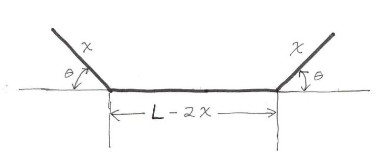
6.4.2 Example 2: Maximize the Cross Sectional Area of a Trough
A long rectangular sheet of aluminum of widthLis to be formed into a flat bottom trough by bending both a left and right hand lengthxup by an angleθwith the horizontal. A cross section view is then:
Figure 8: Flat Bottomed Trough
The lower base isl=L−2 x, the upper base isu=l+2 x cos(θ). The altitude ish=x sin(θ). The area of a trape- zoid whose parallel sides arelanduand whose altitude ish is(h/2) (l+u) (ie., the height times the average width:
Exercise: check this by calculating the area of a rectangeh u, whereuis the larger base, and then subtracting the area of the two similar right triangles on the left and right hand sides.) Hence the area of the cross section (calledsin our Maxima work) isA =L x sin(θ)−2x2 sin(θ) +x2 sin(θ) cos(θ)
Using condition I equations, we proceed to find the extremum solutions forxandθ (which is calledthin our Maxima work). Our method is merely one possible path to a solution.
(%i1) s : L*x*sin(th) - 2*xˆ2*sin(th) + xˆ2*sin(th)*cos(th);
2 2
(%o1) sin(th) x L + cos(th) sin(th) x - 2 sin(th) x (%i2) dsdx : ( diff(s,x), factor(%%) );
(%o2) sin(th) (L + 2 cos(th) x - 4 x)
We see thatone waywe can getdsdxto be zero is to setsin(θ) = 0, however this would mean the angle of bend was zero degrees, which is not the solution of interest. Hence our first equation comes from setting the second factor ofdsdxequal to zero.
(%i3) eq1 : dsdx/sin(th) = 0;
(%o3) L + 2 cos(th) x - 4 x = 0
(%i4) solx : solve(eq1,x);
L
(%o4) [x = - ---]
2 cos(th) - 4 (%i5) dsdth : ( diff(s,th), factor(%%) );
2 2
(%o5) x (cos(th) L - sin (th) x + cos (th) x - 2 cos(th) x)
We see that we can getdsdthto be zero if we setx=0, but this is not the physical situation we are examining. We assume (of course) thatx6=0, and arrive at our second equation of condition I by setting the second factor ofdsdth equal to zero.
(%i6) eq2 : dsdth/x = 0;
2 2
(%o6) cos(th) L - sin (th) x + cos (th) x - 2 cos(th) x = 0 (%i7) eq2 : ( subst(solx,eq2), ratsimp(%%) );
2 2
(sin (th) + cos (th) - 2 cos(th)) L (%o7) --- = 0
2 cos(th) - 4
The only way we can satisfyeq2 is to set the numerator of the left hand side equal to zero, and divide out the factorL which is positive:
(%i8) eq2 : num(lhs(eq2) )/L = 0;
2 2
(%o8) sin (th) + cos (th) - 2 cos(th) = 0 (%i9) eq2 : trigsimp(eq2);
(%o9) 1 - 2 cos(th) = 0
(%i10) solcos : solve( eq2, cos(th) );
1
(%o10) [cos(th) = -]
2 (%i11) solx : subst(solcos, solx);
L
(%o11) [x = -]
3 (%i12) solth : solve(solcos,th);
‘solve’ is using arc-trig functions to get a solution.
Some solutions will be lost.
%pi
(%o12) [th = ---]
3
6.5 Tangent and Normal of a Point of a Curve Defined by an Implicit Function In the following, Maxima assumes thatyis independent ofx:
(%i1) diff(xˆ2 + yˆ2,x);
(%o1) 2 x
We can indicate explicitly thatydepends onxfor purposes of taking this derivative by replacingybyy(x).
(%i2) diff(xˆ2 + y(x)ˆ2,x);
d
(%o2) 2 y(x) (-- (y(x))) + 2 x
dx
Instead of using the functional notation to indicate dependency, we can use thedependsfunction before taking the derivative.
(%i3) depends(y,x);
(%o3) [y(x)]
(%i4) g : diff(xˆ2 + yˆ2, x);
dy
(%o4) 2 y -- + 2 x
dx (%i5) grind(g)$
2*y*’diff(y,x,1)+2*x$
(%i6) gs1 : subst(’diff(y,x) = xˆ3, g );
3
(%o6) 2 x y + 2 x
In%i4 we definedgas the derivative (with respect tox) of the expressionxˆ2 + yˆ2, after telling Maxima that the symbolyis to be considered dependent on the value ofx. Since Maxima, as yet, has no specific information about the nature of the dependence ofyonx, the output is expressed in terms of the ”noun form” ofdiff, which Maxima’s pretty print shows as d yd x. To see the ”internal” form, we again use thegrindfunction, which shows the explicit noun form
’diff(y,x,1). This is useful to know if we want to later replace that unknown derivative with a known result, as we do in input%i6.
However, Maxima doesn’t do anything creative with the derivative substitution done in%i6, like working backwards to what the explicit function ofxthe symbolymight stand for (different answers differ by a constant). The output%o6still contains the symboly.
Two ways to later implement our knowledge ofy(x)are shown in steps%i7and%i8, which use theevfunction. (In Chapter 1 we discussed usingevfor making substitutions, although the use ofsubstis more generally recommended for that job.)
(%i7) ev(g,y=xˆ4/4,diff);
7 x
(%o7) -- + 2 x
2 (%i8) ev(g,y=xˆ4/4,nouns);
7 x
(%o8) -- + 2 x
2 (%i9) y;
(%o9) y
(%i10) g;
dy
(%o10) 2 y -- + 2 x
dx
We see that Maxima does not bind the symbolyto anything when we callevwith an equation likey = xˆ4/4, and that the binding ofghas not changed.
A list which reminds you of all dependencies in force is dependencies. The Maxima functiondiff is the only core function which makes use of thedependencieslist. The functionsintegrateandlaplacedo not use the dependsassignments; one must indicate the dependence explicitly by using functional notation.
In the following, we first ask for the contents of thedependencieslist and then ask Maxima to remove the above dependency ofyonx, usingremove, then check the list contents again, and carry out the previous differentiation with Maxima no longer assuming thatydepends onx.
(%i11) dependencies;
(%o11) [y(x)]
(%i12) remove(y, dependency);
(%o12) done
(%i13) dependencies;
(%o13) []
(%i14) diff(xˆ2 + yˆ2,x);
(%o14) 2 x
On can also remove the properties associated with the symbolyby usingkill (y), although this is more drastic than usingremove.
(%i15) depends(y,x);
(%o15) [y(x)]
(%i16) dependencies;
(%o16) [y(x)]
(%i17) kill(y);
(%o17) done
(%i18) dependencies;
(%o18) []
(%i19) diff(xˆ2+yˆ2,x);
(%o19) 2 x
There are many varieties of using thekillfunction. The way we are using it here corresponds to the syntax:
Function:kill (a_1, ..., a_n)
Removes all bindings (value, function, array, or rule) from the argumentsa_1, ..., a_n. An argumenta_kmay be a symbol or a single array element.
The listdependenciesis one of the lists Maxima uses to hold information introduced during a work session. You can use the commandinfoliststo obtain a list of the names of all of the information lists in Maxima.
(%i1) infolists;
(%o2) [labels, values, functions, macros, arrays, myoptions, props, aliases, rules, gradefs, dependencies, let_rule_packages, structures]
When you first start up Maxima, each of the above named lists is empty.
(%i2) functions;
(%o2) []
6.5.1 Tangent of a Point of a Curve Defined byf(x,y) =0
Suppose some plane curve is defined by the equationf(x,y) =0. Every point(x,y)belonging to the curve must satisfy that equation. For such pairs of numbers, changingxforces a change inyso that the equation of the curve is still satisfied.
When we start plotting tangent lines to plane curves, we will need to evaluate the change iny, given a change inx, such that the numbers(x,y) are always points of the curve. Let’s then regardy as depending onxvia the equation of the curve. Given that the equationf(x,y) =0is valid, we obtain another valid equation by taking the derivative of both sides of the equation with respect tox. Let’s work just on the left hand side of the resulting equation for now:
(%i1) depends(y,x);
(%o1) [y(x)]
(%i2) diff(f(x,y),x);
d
(%o2) -- (f(x, y))
dx
We can make progress by assigning values to the partial derivative off(x,y) with respect to the first argumentx and also to the partial derivative off(x,y)with respect to the second argumenty, using thegradeffunction. The assigned values can be explicit mathematical expressions or symbols. We are going to adopt the symboldfdx to stand for the partial derivative
dfdx=
µ∂f(x,y)
∂x
y
,
where theysubscript means “treatyas a constant when evaluating this derivative”.
Likewise, we will use the symbol dfdy to stand for the partial derivative off(x,y) with respect to y, holdingx constant:
dfdy=
µ∂f(x,y)
∂y
x
.
(%i3) gradef(f(x,y), dfdx, dfdy );
(%o3) f(x, y)
(%i4) g : diff( f(x,y), x );
dy
(%o4) dfdy -- + dfdx
dx (%i5) grind(g)$
dfdy*’diff(y,x,1)+dfdx$
(%i6) g1 : subst(’diff(y,x) = dydx, g);
(%o6) dfdy dydx + dfdx
We have adopted the symboldydxfor the “rate of change” ofyasxvaries, subject to the constraint that the numbers (x,y)always satisfy the equation of the curvef(x,y) =0, which implies thatg1 = 0.
(%i7) solns : solve(g1=0, dydx);
dfdx
(%o7) [dydx = - ----]
dfdy
We see that Maxima knows enough about the rules for differentiation to allow us to get to a famous calculus formula. If xandyare constrained by the equationf(x,y) =0, then the “slope” of the local tangent to the point(x,y)is
d y d x = −
³
∂f(x,y)∂x
´
³
y∂f(x,y)
∂y
´
x
. (6.8)
Of course, this formal expression has no meaning at a point where the denominator is zero.
In your calculus book you will find the derivation of the differentiation rule embodied in our output%o4above:
d
d x f (x, y(x)) =
µ ∂f (x, y)
∂x
y
+
µ ∂f (x, y)
∂y
x
d y(x)
d x (6.9)
Remember that Maxima knows only what the code writers put in; we normally assume that the correct laws of mathemat- ics are encoded as an aid to calculation. If Maxima were not consistent with the differentiation rule Eq. (6.9), then a bug would be present and would have to be removed.
The result Eq.(6.8) provides a way to find the slope (which we callm) at a general point(x,y).
This “slope” should be evaluated at the curve point(x0,y0)of interest to get the tangent and normal in numerical form. Recall our discussion in the first part of Section(6.3) where we derived the relation between the slopes of the tangent and normal. If the numerical value of the slope ism0, then the tangent (line) is the equationy=m0(x−x0) +y0, and the normal (line) is the equationy=−(x−x0)/m0+y0
A Function which Solves ford y/d xgiven thatf(x,y) =0
Given an equation relatingxandy, we assume we can rewrite that equation in the formf(x,y) =0, and then define the following function:
(%i1) dydx(expr,x,y) := -diff(expr,x)/diff(expr,y);
- diff(expr, x) (%o1) dydx(expr, x, y) := ---
diff(expr, y)
As a first example, consider findingd y/d xgiven thatx3+y3=1.
(%i2) dydx( xˆ3+yˆ3-1,x,y);
2 x
(%o2) - --
2 y
Next findd y/d xgiven thatcos(x2−y2) =ycos(x).
(%i3) r1 : dydx( cos(xˆ2 - yˆ2) - y*cos(x),x,y );
2 2
- 2 x sin(y - x ) - sin(x) y (%o3) ---
2 2
- 2 y sin(y - x ) - cos(x) (%i4) r2 : (-num(r1))/(-denom(r1));
2 2
2 x sin(y - x ) + sin(x) y
(%o4) ---
2 2
2 y sin(y - x ) + cos(x)
Maxima does not simplifyr1by cancelling the minus signs automatically, and we have resorted to dividing the negative of the numerator by the negative of the denominator(!) to get the form ofr2. Notice also that Maxima has chosen to writesin(y2−x2)instead ofsin(x2−y2).
Finally, findd y/d xgiven that3 y4+4 x−x2sin(y)−4=0.
(%i5) dydx(3*yˆ4 +4*x -xˆ2*sin(y) - 4, x, y );
2 x sin(y) - 4
(%o5) ---
3 2
12 y - x cos(y)
6.5.2 Example 1: Tangent and Normal of a Point of a Circle
As an easy first example, lets consider a circle of radiusrdefined by the equationx2+y2 =r2. Let’s chooser=1.
Thenf(x,y) =x2+y2−1=0defines the circle of interest, and we use the “slope” function above to calculate the slopemfor a general point(x,y).
(%i1) dydx(expr,x,y) := -diff(expr,x)/diff(expr,y)$
(%i2) f:xˆ2 + yˆ2-1$
(%i3) m : dydx(f,x,y);
x
(%o3) - -
y
![Figure 1: Plot of g over the range [−4, 4]](https://thumb-eu.123doks.com/thumbv2/1library_info/4347599.1574540/8.918.235.695.162.510/figure-plot-g-range.webp)