Ch. 3, Ordinary Differential Equation Tools
∗Edwin L. Woollett December 21, 2017
Contents
3.1 Solving Ordinary Differential Equations . . . 3
3.2 Solution of One First Order Ordinary Differential Equation (ODE) . . . 3
3.2.1 Summary Table . . . 3
3.2.2 Exact Solution with ode2 and ic1 . . . . 3
3.2.3 Exact Solution Using desolve . . . . 5
3.2.4 Numerical Solution and Plot with plotdf . . . 6
3.2.5 Numerical Solution with 4th Order Runge-Kutta: rk . . . . 7
3.3 Solution of One Second Order ODE or Two First Order ODE’s . . . 9
3.3.1 Summary Table . . . 9
3.3.2 Exact Solution with ode2, ic2, and eliminate . . . . 9
3.3.3 Exact Solution with desolve, atvalue, and eliminate . . . . 12
3.3.4 Numerical Solution and Plot with plotdf . . . 16
3.3.5 Numerical Solution with 4th Order Runge-Kutta: rk . . . . 17
3.4 Examples of ODE Solutions . . . 19
3.4.1 Ex. 1: Fall in Gravity with Air Friction: Terminal Velocity . . . 19
3.4.2 Ex. 2: One Nonlinear First Order ODE . . . 22
3.4.3 Ex. 3: One First Order ODE Which is Not Linear in Y’ . . . 23
3.4.4 Ex. 4: Linear Oscillator with Damping . . . 24
3.4.5 Ex. 5: Underdamped Linear Oscillator with Sinusoidal Driving Force . . . 28
3.4.6 Ex. 6: Regular and Chaotic Motion of a Driven Damped Planar Pendulum . . . 30
3.4.7 Free Oscillation Case . . . 31
3.4.8 Damped Oscillation Case . . . 32
3.4.9 Including a Sinusoidal Driving Torque . . . 33
3.4.10 Regular Motion Parameters Case . . . 33
3.4.11 Chaotic Motion Parameters Case. . . 37
3.5 Using contrib ode for ODE’s . . . 43
∗This version uses Maxima 5.18.1 Check http://www.csulb.edu/˜woollett/ for the latest version of these notes. Send comments and suggestions towoollett@charter.net
1
This document is part of a series of notes titled
"Maxima by Example" and is made available
via the author’s webpage http://www.csulb.edu/˜woollett/
to aid new users of the Maxima computer algebra system.
NON-PROFIT PRINTING AND DISTRIBUTION IS PERMITTED.
You may make copies of this document and distribute them
to others as long as you charge no more than the costs of printing.
These notes (with some modifications) will be published in book form eventually via Lulu.com in an arrangement which will continue
to allow unlimited free download of the pdf files as well as the option of ordering a low cost paperbound version of these notes.
Feedback from readers is the best way for this series of notes to become more helpful to new users of Maxima. All comments and suggestions for improvements will be appreciated and carefully considered.
LOADING FILES
The defaults allow you to use the brief version load(fft) to load in the Maxima file fft.lisp.
To load in your own file, such as qxxx.mac
using the brief version load(qxxx), you either need to place qxxx.mac in one of the folders Maxima searches by default, or else put a line like:
file_search_maxima : append(["c:/work2/###.{mac,mc}"],file_search_maxima )$
in your personal startup file maxima-init.mac (see later in this chapter for more information about this).
Otherwise you need to provide a complete path in double quotes, as in load("c:/work2/qxxx.mac"),
We always use the brief load version in our examples, which are generated using the XMaxima graphics interface on a Windows XP computer, and copied into a fancy verbatim environment in a latex file which uses the fancyvrb and color packages.
Maxima.sourceforge.net. Maxima, a Computer Algebra System. Version 5.18.1 (2009). http://maxima.sourceforge.net/
The homemade functionfll(x)(first, last, length) is used to return the first and last elements of lists (as well as the length), and is automatically loaded in withmbe1util.macfrom Ch. 1. We will include a reference to this definition when working with lists.
This function has the definitions
fll(x) := [first(x),last(x),length(x)]$
declare(fll,evfun)$
Some of the examples used in these notes are from the Maxima html help manual or the Maxima mailing list:
http://maxima.sourceforge.net/maximalist.html.
The author would like to thank the Maxima developers for their friendly help via the Maxima mailing list.
2
3.1 Solving Ordinary Differential Equations
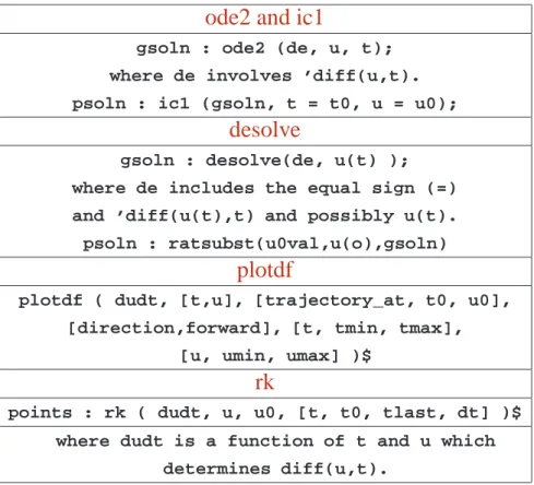
3.2 Solution of One First Order Ordinary Differential Equation (ODE) 3.2.1 Summary Table
ode2 and ic1
gsoln : ode2 (de, u, t);
where de involves ’diff(u,t).
psoln : ic1 (gsoln, t = t0, u = u0);
desolve
gsoln : desolve(de, u(t) );
where de includes the equal sign (=) and ’diff(u(t),t) and possibly u(t).
psoln : ratsubst(u0val,u(o),gsoln)
plotdf
plotdf ( dudt, [t,u], [trajectory_at, t0, u0], [direction,forward], [t, tmin, tmax],
[u, umin, umax] )$
rk
points : rk ( dudt, u, u0, [t, t0, tlast, dt] )$
where dudt is a function of t and u which determines diff(u,t).
Table 1: Methods for One First Order ODE
We will use these four different methods to solve the first order ordinary differential equation d u
d t =e−t+u (3.1)
subject to the condition that whent=2, u=−0.1.
3.2.2 Exact Solution with ode2 and ic1
Most ordinary differential equations have no known exact solution (or the exact solution is a complicated expression involving many terms with special functions) and one normally uses approximate methods. However, some ordinary differential equations have simple exact solutions, and many of these can be found using ode2, desolve, or contrib ode.
The manual has the following information about ode2 Function: ode2 (eqn, dvar, ivar)
The function ode2 solves an ordinary differential equation (ODE) offirst or second order. It takes three arguments: an ODE given by eqn, the dependent variable dvar, and the independent variable ivar. When successful, it returns either an explicit or implicit solution for the dependent variable.%cis used to represent the integration constant in the case of first-order equations, and%k1and%k2the constants for second-order equations. The dependence of the dependent variable on the independent variable does not have to be written explicitly, as in the case of desolve, but the independent variable must always be given as the third argument.
If the differential equation has the structure Left(dudt,u,t) = Right(dudt,u,t) ( here u is the dependent variable and t is the independent variable), we can always rewrite that differential equation as de = Left(dudt,u,t) - Right(dudt,u,t) = 0, or de = 0.
We can use the syntax ode2(de,u,t), with the first argument an expression which includes derivatives, instead of the com- plete equation including the ” = 0” on the end, and ode2 will assume we mean de = 0 for the differential equation. (Of course you can also use ode2 ( de=0, u, t)
We rewrite our example linear first order differential equation Eq. 3.1 in the way just described, using the noun form
’diff, which uses a single quote. We then use ode2, and call the general solution gsoln.
(%i1) de : ’diff(u,t)- u - exp(-t);
du - t
(%o1) -- - u - %e
dt (%i2) gsoln : ode2(de,u,t);
- 2 t
%e t
(%o2) u = (%c - ---) %e
2
The general solution returned by ode2 contains one constant of integration%c, and is an explicit solution for u as a func- tion of t, although the above does not bind the symbolu.
We next find the particular solution which hast=2, u=−0.1 using ic1, and call this particular solution psoln. We then check the returned solution in two ways: 1. does it satisfy the conditions given to ic1?, and 2. does it produce a zero value for our expression de?
(%i3) psoln : ic1(gsoln,t = 2, u = -0.1),ratprint:false;
- t - 4 2 2 t 4
%e ((%e - 5) %e + 5 %e ) (%o3) u = - ---
10 (%i4) rhs(psoln),t=2,ratsimp;
1
(%o4) - --
10 (%i5) de,psoln,diff,ratsimp;
(%o5) 0
Both tests are passed by this particular solution. We can now make a quick plot of this solution using plot2d.
(%i6) us : rhs(psoln);
- t - 4 2 2 t 4
%e ((%e - 5) %e + 5 %e ) (%o6) - ---
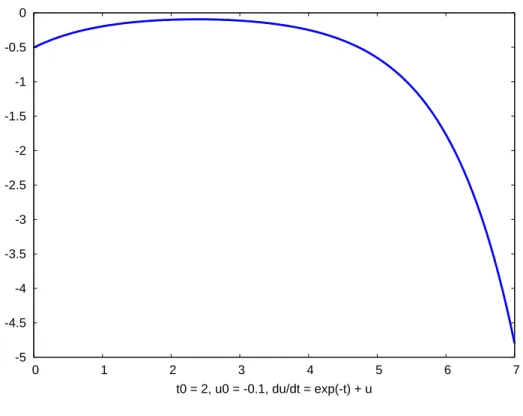
10 (%i7) plot2d(us,[t,0,7],
[style,[lines,5]],[ylabel," "],
[xlabel,"t0 = 2, u0 = -0.1, du/dt = exp(-t) + u"])$
which looks like
-5 -4.5 -4 -3.5 -3 -2.5 -2 -1.5 -1 -0.5 0
0 1 2 3 4 5 6 7
t0 = 2, u0 = -0.1, du/dt = exp(-t) + u
Figure 1: Solution for whicht=2, u=−0.1
3.2.3 Exact Solution Using desolve
desolve uses Laplace transform methods to find an exact solution. To be able to use desolve, we need to write our example differential equation Eq.3.1 in a more explicit form, with everyu -> u(t), and include the=sign in the definition of the differential equation.
(%i1) eqn : ’diff(u(t),t) - exp(-t) - u(t) = 0;
d - t
(%o1) -- (u(t)) - u(t) - %e = 0
dt (%i2) gsoln : desolve(eqn,u(t));
t - t
(2 u(0) + 1) %e %e
(%o2) u(t) = --- - ---
2 2
(%i3) eqn,gsoln,diff,ratsimp;
(%o3) 0 = 0
(%i4) bc : subst ( t=2, rhs(gsoln)) = - 0.1;
2 - 2
%e (2 u(0) + 1) %e
(%o4) --- - --- = - 0.1
2 2
(%i5) solve ( eliminate ( [gsoln, bc],[u(0)]), u(t) ),ratprint:false;
- t t - 2 t - 4
- 5 %e - %e + 5 %e (%o5) [u(t) = ---]
10 (%i6) us : rhs(%[1]);
- t t - 2 t - 4
- 5 %e - %e + 5 %e
(%o6) ---
10
(%i7) us, t=2, ratsimp;
1
(%o7) - --
10 (%i8) plot2d(us,[t,0,7],
[style,[lines,5]],[ylabel," "],
[xlabel,"t0 = 2, u0 = -0.1, du/dt = exp(-t) + u"])$
and we get the same plot as before. The function desolve returns a solution in terms of the “initial value”u(0), which here meansu(t = 0), and we must go through an extra step to eliminateu(0)in a way that assures our chosen bound- ary conditiont = 2, u - -0.1is satisfied.
We have checked that the general solution satisfies the given differential equation in %i3, and have checked that our particular solution satisfies the desired condition att = 2in%i7.
If your problem requires that the value of the solutionusbe specified att = 0, the route to the particular solution is much simpler than what we used above. You simply usesubst ( u(0) = -1, rhs (gsoln) )if, for example, you wanted a particular solution to have the property that whent = 0,u = -1.
(%i9) us : subst( u(0) = -1,rhs(gsoln) ),ratsimp;
- t 2 t
%e (%e + 1)
(%o9) - ---
2 (%i10) us,t=0,ratsimp;
(%o10) - 1
3.2.4 Numerical Solution and Plot with plotdf
We next use plotdf to numerically integrate the given first order ordinary differential equation, draw a direction field plot which governs any particular solution, and draw the particular solution we have chosen.
The default color choice of plotdf is to use small blue arrows give the local direction of the trajectory of the partic- ular solution passing though that point. This direction can be defined by an angle α such that if u′ =f(t,u), then tan(α) =f(t,u), and at the point(t0,u0),
d u=f(t0,u0)× d t=d t ×
d u
d t
t=t0,u=u0
(3.2) This equation determines the increase d u in the value of the dependent variable u induced by a small increase d t in the independent variable t at the point(t0,u0). We then define a local vector with t component d t and u component d u, and draw a small arrow in that direction at a grid of chosen points to construct a direction field associated with the given first order differential equation. The length of the small arrow can be increased some to reflect large values of the magnitude ofd u/d t.
For one first order ordinary differential equation, plotdf, has the syntax
plotdf( dudt,[t,u], [trajectory_at, t0, u0], options ... )
in whichdudtis the function of(t,u)which determines the rate of changed u/d t.
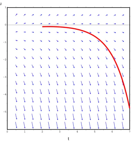
(%i1) plotdf(exp(-t) + u, [t, u], [trajectory_at,2,-0.1], [direction,forward], [t,0,7], [u, -6, 1] )$
produces the plot
0 1 2 3 4 5 6 7
-5 -4 -3 -2 -1 0 1
u
t
Figure 2: Direction Field for the Solutiont=2, u=−0.1
(We have thickened the red curve using the Config, Linewidth menu option of plotdf, followed by Replot).
The help manual has an extensive discussion and examples of the use of the direction field plot utility plotdf.
3.2.5 Numerical Solution with 4th Order Runge-Kutta: rk
Although the plotdf function is useful for orientation about the shapes and types of solutions possible, if you need a list with coordinate points to use for other purposes, you can use the fourth order Runge-Kutta function rk.
For one first order ordinary differential equation, the syntax has some faint resemblance to that of plotdf:
rk ( dudt, u, u0, [ t, t0, tlast, dt ] )
in which we are assuming that u is the dependent variable and t is the independent variable, anddudtis that function of (t, u) which locally determines the value ofd u/d t. This will numerically integrate the corresponding first order ordinary differential equation and return a list of pairs of (t, u) on the solution curve which has been requested:
[ [t0, u0], [t0 + dt, y(t0 + dt)], .... ,[tlast, y(tlast)] ]
For our example first order ordinary differential equation, choosing the same initial conditions as above, and choosing dt = 0.01,
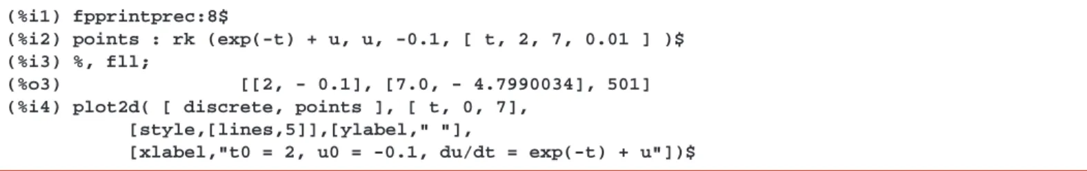
(%i1) fpprintprec:8$
(%i2) points : rk (exp(-t) + u, u, -0.1, [ t, 2, 7, 0.01 ] )$
(%i3) %, fll;
(%o3) [[2, - 0.1], [7.0, - 4.7990034], 501]
(%i4) plot2d( [ discrete, points ], [ t, 0, 7], [style,[lines,5]],[ylabel," "],
[xlabel,"t0 = 2, u0 = -0.1, du/dt = exp(-t) + u"])$
(We have used our homemade functionfll(x), loaded in at startup with the other functions defined inmbe1util.mac, available with the Ch. 1 material. We have provided the definition offllin the preface of this chapter. Instead of
%, fll ;, you could use[%[1],last(%),length(%)];to get the same information.) The plot looks like
-5 -4.5 -4 -3.5 -3 -2.5 -2 -1.5 -1 -0.5 0
2 3 4 5 6 7
t0 = 2, u0 = -0.1, du/dt = exp(-t) + u
Figure 3: Runge-Kutta Solution witht=2, u=−0.1
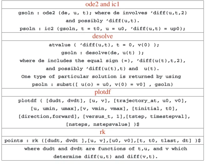
3.3 Solution of One Second Order ODE or Two First Order ODE’s 3.3.1 Summary Table
ode2 and ic1
gsoln : ode2 (de, u, t); where de involves ’diff(u,t,2) and possibly ’diff(u,t).
psoln : ic2 (gsoln, t = t0, u = u0, ’diff(u,t) = up0);
desolve
atvalue ( ’diff(u,t), t = 0, v(0) );
gsoln : desolve(de, u(t) );
where de includes the equal sign (=), ’diff(u(t),t,2), and possibly ’diff(u(t),t) and u(t).
One type of particular solution is returned by using psoln : subst([ u(o) = u0, v(0) = v0] , gsoln)
plotdf
plotdf ( [dudt, dvdt], [u, v], [trajectory_at, u0, v0], [u, umin, umax],[v, vmin, vmax], [tinitial, t0], [direction,forward], [versus_t, 1],[tstep, timestepval],
[nsteps, nstepsvalue] )$
rk
points : rk ([dudt, dvdt ],[u, v],[u0, v0],[t, t0, tlast, dt] )$
where dudt and dvdt are functions of t,u, and v which determine diff(u,t) and diff(v,t).
Table 2: Methods for One Second Order or Two First Order ODE’s We apply the above four methods to the simple second order ordinary differential equation:
d2u
d t2 =4 u (3.3)
subject to the conditions that whent=2,u=1andd u/d t =0.
3.3.2 Exact Solution with ode2, ic2, and eliminate The main difference here is the use of ic2 rather than ic1.
(%i1) de : ’diff(u,t,2) - 4*u;
2 d u
(%o1) --- - 4 u
2 dt (%i2) gsoln : ode2(de,u,t);
2 t - 2 t
(%o2) u = %k1 %e + %k2 %e
(%i3) de,gsoln,diff,ratsimp;
(%o3) 0
(%i4) psoln : ic2(gsoln,t=2,u=1,’diff(u,t) = 0);
2 t - 4 4 - 2 t
%e %e
(%o4) u = --- + ---
2 2
(%i5) us : rhs(psoln);
2 t - 4 4 - 2 t
%e %e
(%o5) --- + ---
2 2
(%i6) us, t=2, ratsimp;
(%o6) 1
(%i7) plot2d(us,[t,0,4],[y,0,10],
[style,[lines,5]],[ylabel," "],
[xlabel," U versus t, U’’(t) = 4 U(t), U(2) = 1, U’(2) = 0 "])$
plot2d: expression evaluates to non-numeric value somewhere in plotting range.
which produces the plot
0 2 4 6 8 10
0 0.5 1 1.5 2 2.5 3 3.5 4
U versus t, U’’(t) = 4 U(t), U(2) = 1, U’(2) = 0
Figure 4: Solution for whicht=2, u=1, u′ =0
Next we make a “phase space plot” which is a plot ofv=d u/d tversusuover the range1≤t≤3.
(%i8) vs : diff(us,t),ratsimp;
- 2 t - 4 4 t 8
(%o8) %e (%e - %e )
(%i9) for i thru 3 do
d[i]:[discrete,[float(subst(t=i,[us,vs]))]]$
(%i10) plot2d( [[parametric,us,vs,[t,1,3]],d[1],d[2],d[3] ], [x,0,8],[y,-12,12],
[style, [lines,5,1],[points,4,2,1], [points,4,3,1],[points,4,6,1]], [ylabel," "],[xlabel," "],
[legend," du/dt vs u "," t = 1 ","t = 2","t = 3"] )$
which produces the plot
-10 -5 0 5 10
0 1 2 3 4 5 6 7 8
du/dt vs u t = 1 t = 2 t = 3
Figure 5: t=2, y=1, y′=0Solution
If your boundary conditions are, instead, fort=0, u = 1, and for t = 2, u = 4, then one can eliminate the two constants “by hand” instead of using ic2 (see also next section).
(%i4) bc1 : subst(t=0,rhs(gsoln)) = 1$
(%i5) bc2 : subst(t = 2, rhs(gsoln)) = 4$
(%i6) solve(
eliminate([gsoln,bc1,bc2],[%k1,%k2]), u ), ratsimp, ratprint:false;
- 2 t 4 4 t 8 4
%e ((4 %e - 1) %e + %e - 4 %e ) (%o6) [u = ---]
8
%e - 1 (%i7) us : rhs(%[1]);
- 2 t 4 4 t 8 4
%e ((4 %e - 1) %e + %e - 4 %e ) (%o7) ---
8
%e - 1 (%i8) us,t=0,ratsimp;
(%o8) 1
(%i9) us,t=2,ratsimp;
(%o9) 4
3.3.3 Exact Solution with desolve, atvalue, and eliminate
The function desolve uses Laplace transform methods which are set up to expect the use of initial values for dependent variables and their derivatives. (However, we will show how you can impose more general boundary conditions.) If the dependent variable isu(t), for example, the solution is returned in terms of a constantu(0), which refers to the value ofu(t = 0)(here we are assuming that the independent variable ist). To get a simple result from desolve which we can work with (for the case of a second order ordinary differential equation), we can use the atvalue function with the syntax (for example):
atvalue ( ’diff(u,t), t = 0, v(0) )
which will allow desolve to return the solution to a second order ODE in terms of the pair of constants( u(0), v(0) ).
Of course, there is nothing sacred about using the symbolv(0)here. The function atvalue should be invoked before the use of desolve.
If the desired boundary conditions for a particular solution refer tot = 0, then you can immediately find that particular solution using the syntax (ifugis the general solution, say)
us : subst( [ u(0) = u0val, v(0) = v0val], ug ),
or else by using ratsubst twice.
In our present example, the desired boundary conditions refer to t = 2 , and impose conditions on the value of u and its first derivative at that value oft. This requires a little more work, and we use eliminate to get rid of the constants (u(0), v(0))in a way that allows our desired conditions to be satisfied.
(%i1) eqn : ’diff(u(t),t,2) - 4*u(t) = 0;
2 d
(%o1) --- (u(t)) - 4 u(t) = 0
2 dt
(%i2) atvalue ( ’diff(u(t),t), t=0, v(0) )$
(%i3) gsoln : desolve(eqn,u(t));
2 t - 2 t
(v(0) + 2 u(0)) %e (v(0) - 2 u(0)) %e (%o3) u(t) = --- - ---
4 4
(%i4) eqn,gsoln,diff,ratsimp;
(%o4) 0 = 0
(%i5) ug : rhs(gsoln);
2 t - 2 t
(v(0) + 2 u(0)) %e (v(0) - 2 u(0)) %e (%o5) --- - ---
4 4
(%i6) vg : diff(ug,t),ratsimp$
(%i7) ubc : subst(t = 2,ug) = 1$
(%i8) vbc : subst(t = 2,vg) = 0$
(%i9) solve (
eliminate([gsoln, ubc, vbc],[u(0), v(0)]), u(t) ), ratsimp,ratprint:false;
- 2 t - 4 4 t 8
%e (%e + %e )
(%o9) [u(t) = ---]
2
(%i10) us : rhs(%[1]);
- 2 t - 4 4 t 8
%e (%e + %e )
(%o10) ---
2 (%i11) subst(t=2, us),ratsimp;
(%o11) 1
(%i12) vs : diff(us,t),ratsimp;
- 2 t - 4 4 t 8
(%o12) %e (%e - %e )
(%i13) subst(t = 2,vs),ratsimp;
(%o13) 0
(%i14) plot2d(us,[t,0,4],[y,0,10],
[style,[lines,5]],[ylabel," "],
[xlabel," U versus t, U’’(t) = 4 U(t), U(2) = 1, U’(2) = 0 "])$
plot2d: expression evaluates to non-numeric value somewhere in plotting range.
(%i15) for i thru 3 do
d[i]:[discrete,[float(subst(t=i,[us,vs]))]]$
(%i16) plot2d( [[parametric,us,vs,[t,1,3]],d[1],d[2],d[3] ], [x,0,8],[y,-12,12],
[style, [lines,5,1],[points,4,2,1], [points,4,3,1],[points,4,6,1]], [ylabel," "],[xlabel," "],
[legend," du/dt vs u "," t = 1 ","t = 2","t = 3"] )$
which generates the same plots found with the ode2 method above.
If the desired boundary conditions are that uhave given values at t = 0and t = 3, then we can proceed from the same general solution above as follows withupbeing a partially defined particular solution (assumeu(0) = 1 and u(3) = 2):
(%i17) up : subst(u(0) = 1, ug);
2 t - 2 t
(v(0) + 2) %e (v(0) - 2) %e (%o17) --- - ---
4 4
(%i18) ubc : subst ( t=3, up) = 2;
6 - 6
%e (v(0) + 2) %e (v(0) - 2) (%o18) --- - --- = 2
4 4
(%i19) solve(
eliminate ( [ u(t) = up, ubc ],[v(0)] ), u(t) ), ratsimp, ratprint:false;
- 2 t 6 4 t 12 6
%e ((2 %e - 1) %e + %e - 2 %e ) (%o19) [u(t) = ---]
12
%e - 1 (%i20) us : rhs (%[1]);
- 2 t 6 4 t 12 6
%e ((2 %e - 1) %e + %e - 2 %e ) (%o20) ---
12
%e - 1 (%i21) subst(t = 0, us),ratsimp;
(%o21) 1
(%i22) subst (t = 3, us),ratsimp;
(%o22) 2
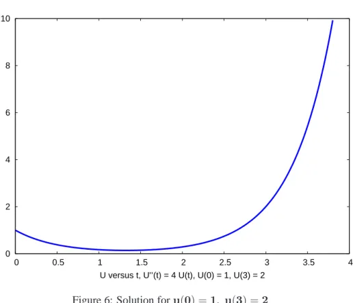
(%i23) plot2d(us,[t,0,4],[y,0,10],
[style,[lines,5]],[ylabel," "],
[xlabel," U versus t, U’’(t) = 4 U(t), U(0) = 1, U(3) = 2 "])$
plot2d: expression evaluates to non-numeric value somewhere in plotting range.
which produces the plot
0 2 4 6 8 10
0 0.5 1 1.5 2 2.5 3 3.5 4
U versus t, U’’(t) = 4 U(t), U(0) = 1, U(3) = 2
Figure 6: Solution foru(0) =1, u(3) =2
If instead, you need to satisfyu(1) = -1andu(3) = 2, you could proceed fromgsolnandugas follows:
(%i24) ubc1 : subst ( t=1, ug) = -1$
(%i25) ubc2 : subst ( t=3, ug) = 2$
(%i26) solve(
eliminate ( [gsoln, ubc1, ubc2],[u(0),v(0)]), u(t) ), ratsimp, ratprint:false;
- 2 t 4 4 t 12 8
%e ((2 %e + 1) %e - %e - 2 %e ) (%o26) [u(t) = ---]
10 2
%e - %e (%i27) us : rhs(%[1]);
- 2 t 4 4 t 12 8
%e ((2 %e + 1) %e - %e - 2 %e ) (%o27) ---
10 2
%e - %e (%i28) subst ( t=1, us), ratsimp;
(%o28) - 1
(%i29) subst ( t=3, us), ratsimp;
(%o29) 2
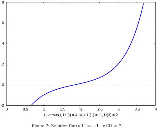
(%i30) plot2d ( us, [t,0,4], [y,-2,8], [style,[lines,5]],[ylabel," "],
[xlabel," U versus t, U’’(t) = 4 U(t), U(1) = -1, U(3) = 2 "])$
which produces the plot
-2 0 2 4 6 8
0 0.5 1 1.5 2 2.5 3 3.5 4
U versus t, U’’(t) = 4 U(t), U(1) = -1, U(3) = 2
Figure 7: Solution foru(1) =−1, u(3) =2
The simplest case of using desolve is the case in which you impose conditions on the solution and its first derivative at t = 0, in which case you simply use:
(%i4) psoln : subst([u(0) = 1,v(0)=0],gsoln);
2 t - 2 t
%e %e
(%o4) u(t) = --- + ---
2 2
(%i5) us : rhs(psoln);
2 t - 2 t
%e %e
(%o5) --- + ---
2 2
in which we have chosen the initial conditionsu(0) = 1, andv(0) = 0.
3.3.4 Numerical Solution and Plot with plotdf
Given a second order autonomous ODE, one needs to introduce a second dependent variablev(t), say, which is defined as the first derivative of the original single dependent variableu(t). Then for our example, the starting ODE
d2u
d t2 =4 u (3.4)
is converted into two first order ODE’s
d u
d t =v, d v
d t =4 u (3.5)
and the plotdf syntax for two first order ODE’s is
plotdf ( [dudt, dvdt], [u, v], [trajectory_at, u0, v0], [u, umin, umax], [v, vmin, vmax], [tinitial, t0], [versus_t, 1],
[tstep, timestepval], [nsteps, nstepsvalue] )$
in which att = t0, u = u0and v = v0. If t0 = 0you can omit the option [tinitial, t0]. The options [u, umin, umax]and [v, vmin, vmax]allow you to control the horizontal and vertical extent of the phase space plot (herevversusu) which will be produced. The option[versus_t,1]tells plotdf to create a separate plot of bothuandvversus the dependent variable. The last two options are only needed if you are not satisfied with the plots and want to experiment with other than the default values oftstepandnsteps.
Another option you can add is[direction,forward], which will display the trajectory fortgreater than or equal tot0, rather than for a default interval around the valuet0which corresponds to[direction,both].
Here we invoke plotdf for our example.
(%i1) plotdf ( [v, 4*u], [u, v], [trajectory_at, 1, 0], [u, 0, 8], [v, -10, 10], [versus_t, 1],
[tinitial, 2])$
The plot versustis
0.8 1.2 1.6 2 2.4 2.8 3.2
-8 -4 0 4 8
u v
t
Figure 8: u(t) and u’(t) vs.tforu(2) =1, u′(2) =0
and the phase space plot is
1 2 3 4 5 6 7
-8 -4 0 4 8
v
u
Figure 9: u’(t) vs. u(t) foru(2) =1, u′(2) =0
In both of these plots we used theConfigmenu to increase the linewidth, and then clicked onReplot. We also cut and pasted the colorredto be the second choice on the color cycle (instead of green) used in the plot versus the independent variablet. Note that no matter what you call your independent variable, it will always be called ton the plot of the dependent variables versus the independent variable.
3.3.5 Numerical Solution with 4th Order Runge-Kutta: rk
To use the fourth order Runge-Kutta numerical integrator rk for this example, we need to follow the procedure used in the previous section using plotdf, converting the second order ODE to a pair of first order ODE’s.
The syntax for two first order ODE’s with dependent variables[u,v]and independent variabletis rk ( [ dudt, dvdt ], [u,v], [u0,v0], [t, t0, tmax, dt] )
which will produce the list of lists:
[ [t0, u0,v0],[t0+dt, u(t0+dt),v(t0+dt)], ..., [tmax, u(tmax),v(tmax)] ]
For our example, following our discussion in the previous section with plotdf, we use points : rk ( [v, 4*u], [u, v], [1, 0], [t, 2, 3.6, 0.01] )
We again use the homemade functionfll(see the preface) to look at the first element, the last element, and the length of various lists.
(%i1) fpprintprec:8$
(%i2) points : rk([v,4*u],[u,v],[1,0],[t,2,3.6,0.01])$
(%i3) %, fll;
(%o3) [[2, 1, 0], [3.6, 12.286646, 24.491768], 161]
(%i4) uL : makelist([points[i][1],points[i][2]],i,1,length(points))$
(%i5) %, fll;
(%o5) [[2, 1], [3.6, 12.286646], 161]
(%i6) vL : makelist([points[i][1],points[i][3]],i,1,length(points))$
(%i7) %, fll;
(%o7) [[2, 0], [3.6, 24.491768], 161]
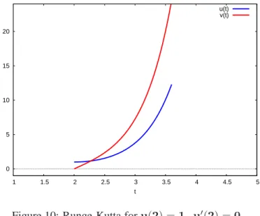
(%i8) plot2d([ [discrete,uL],[discrete,vL]],[x,1,5], [style,[lines,5]],[y,-1,24],[ylabel," "], [xlabel,"t"],[legend,"u(t)","v(t)"])$
which produces the plot
0 5 10 15 20
1 1.5 2 2.5 3 3.5 4 4.5 5
t
u(t) v(t)
Figure 10: Runge-Kutta foru(2) =1, u′(2) =0
Next we make a phase space plot ofvversusufrom the result of the Runge-Kutta integration.
(%i9) uvL : makelist([points[i][2],points[i][3]],i,1,length(points))$
(%i10) %, fll;
(%o10) [[1, 0], [12.286646, 24.491768], 161]
(%i11) plot2d( [ [discrete,uvL]],[x,0,13],[y,-1,25], [style,[lines,5]],[ylabel," "], [xlabel," v vs. u "])$
which produces the phase space plot
0 5 10 15 20 25
0 2 4 6 8 10 12
v vs. u
Figure 11: R-K Phase Space Plot foru(2) =1, u′(2) =0
3.4 Examples of ODE Solutions
3.4.1 Ex. 1: Fall in Gravity with Air Friction: Terminal Velocity
Let’s explore a problem posed by Patrick T. Tam (A Physicist’s Guide to Mathematica, Academic Press, 1997, page 349).
A small body falls downward with an initial velocityv0 from a height hnear the surface of the earth. For low velocities (less than about 24 m/s), the effect of air resistance may be approximated by a frictional force proportional to the velocity. Find the displacement and velocity of the body, and determine the terminal velocity. Plot the speed as a function of time for several initial velocities.
The net vector forceFacting on the object is thus assumed to be the (constant) force of gravity and the (variable) force due to air friction, which is in a direction opposite to the direction of the velocity vectorv. We can then write Newton’s Law of motion in the form
F=mg−bv=mdv
d t (3.6)
In this vector equation, m is the mass in kg., g is a vector pointing downward with magnitude g, and bis a positive constant which depends on the size and shape of the object and on the viscosity of the air. The velocity vectorvpoints down during the fall.
If we choose theyaxis positive downward, with the pointy= 0the launch point, then the netycomponents of the force and Newton’s Law of motion are:
Fy =m g−b vy =md vy
d t (3.7)
wheregis the positive number 9.8m/s2 and since the velocity component vy >0during the fall, the effects of gravity and air resistance are in competition.
We see that the rate of change of velocity will become zero at the instant thatm g−b vy = 0, orvy = m g/b, and the downward velocity stops increasing at that moment, the ”terminal velocity” having been attained.
While working with Maxima, we can simplify our notation and letvy → v and (b/m) → aso bothv andarepresent positive numbers. We then use Maxima to solve the equationd v/d t = g−a v. The dimension of each term of this equation must evidently be the dimension ofv/t, soahas dimension1/t.
(%i1) de : ’diff(v,t) - g + a*v;
dv
(%o1) -- + a v - g
dt (%i2) gsoln : ode2(de,v,t);
a t - a t g %e
(%o2) v = %e (--- + %c)
a (%i3) de, gsoln, diff,ratsimp;
(%o3) 0
We then use ic1 to get a solution such thatv=v0whent= 0.
(%i4) psoln : expand ( ic1 (gsoln,t = 0, v = v0 ) );
- a t
- a t g %e g
(%o4) v = %e v0 - --- + -
a a
(%i5) vs : rhs(psoln);
- a t
- a t g %e g
(%o5) %e v0 - --- + -
a a
For consistency, we must get the correct terminal speed for larget:
(%i6) assume(a>0)$
(%i7) limit( vs, t, inf );
g
(%o7) -
a
which agrees with our analysis.
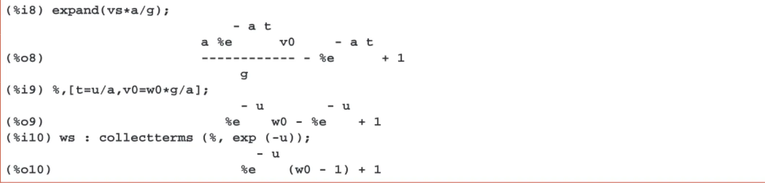
To make some plots, we can introduce a dimensionless timeuwith the replacement t → u =a t, and a dimensionless speedwwith the replacementv→w=a v/g.
(%i8) expand(vs*a/g);
- a t
a %e v0 - a t
(%o8) --- - %e + 1
g (%i9) %,[t=u/a,v0=w0*g/a];
- u - u
(%o9) %e w0 - %e + 1
(%i10) ws : collectterms (%, exp (-u));
- u
(%o10) %e (w0 - 1) + 1
As our dimensionless timeugets large,ws→1, which is the value of the terminal speed in dimensionless units.
Let’s now plot three cases, two cases with initial speed less than terminal speed and one case with initial speed greater than the terminal speed. (The use of dimensionless units for plots generates what are called “universal curves”, since they are generally valid, no matter what the actual numbers are).
(%i11) plot2d([[discrete,[[0,1],[5,1]]],subst(w0=0,ws),subst(w0=0.6,ws), subst(w0=1.5,ws)],[u,0,5],[y,0,2],
[style,[lines,2,7],[lines,4,1],[lines,4,2],[lines,4,3]], [legend,"terminal speed", "w0 = 0", "w0 = 0.6", "w0 = 1.5"], [ylabel, " "],
[xlabel, " dimensionless speed w vs dimensionless time u"])$
which produces:
0 0.5 1 1.5 2
0 1 2 3 4 5
dimensionless speed w vs dimensionless time u terminal speed
w0 = 0 w0 = 0.6 w0 = 1.5
Figure 12: Dimensionless Speed Versus Dimensionless Time
An object thrown down with an initial speed greater than the terminal speed (as in the top curve) slows down until its speed is the terminal speed.
Thus far we have been only concerned with the relation between velocity and time. We can now focus on the implications for distance versus time. A dimensionless lengthz isa2y/g and the relation d y/d t =vbecomes d z/d u=w, or d z=w d u, which can be integrated over corresponding intervals: zover the interval [0,zf], and uover the interval [0,uf].
(%i12) integrate(1,z,0,zf) = integrate(ws,u,0,uf);
- uf uf
(%o12) zf = - %e (w0 - uf %e - 1) + w0 - 1 (%i13) zs : expand(rhs(%)),uf = u;
- u - u
(%o13) - %e w0 + w0 + %e + u - 1
(%i14) zs, u=0;
(%o14) 0
(Remember the object is launched at y=0 which means at z=0). Let’s make a plot of distance travelled vs time (dimensionless units) for the three cases considered above.
(%i15) plot2d([subst(w0=0,zs),subst(w0=0.6,zs),
subst(w0=1.5,zs)],[u,0,1],[style,[lines,4,1],[lines,4,2],
[lines,4,3]], [legend,"w0 = 0", "w0 = 0.6", "w0 = 1.5"], [ylabel," "],
[xlabel,"dimensionless distance z vs dimensionless time u"], [gnuplot_preamble,"set key top left;"])$
which produces:
0 0.2 0.4 0.6 0.8 1 1.2 1.4
0 0.2 0.4 0.6 0.8 1
dimensionless distance z vs dimensionless time u w0 = 0
w0 = 0.6 w0 = 1.5
Figure 13: Dimensionless Distance Versus Dimensionless Time
3.4.2 Ex. 2: One Nonlinear First Order ODE Let’s solve
x2yd y
d x =x y2+x3−1 (3.8)
for a solution such that whenx=1, y=1.
(%i1) de : xˆ2*y*’diff(y,x) - x*yˆ2 - xˆ3 + 1;
2 dy 2 3
(%o1) x y -- - x y - x + 1
dx (%i2) gsoln : ode2(de,y,x);
2 3
3 x y - 6 x log(x) - 2
(%o2) --- = %c
3 6 x (%i3) psoln : ic1(gsoln,x=1,y=1);
2 3
3 x y - 6 x log(x) - 2 1
(%o3) --- = -
3 6
6 x
This implicitly determinesyas a function of the independent variablexBy inspection, we see that x=0 is a singular point we should stay away from, so we assume from now on thatx6=0.
To look atexplicitsolutions y(x) we use solve, which returns a list of two expressions depending on x. Since theimplicit solution is a quadratic in y, we will get two solutions from solve, which we call y1 and y2.
(%i4) [y1,y2] : map(’rhs, solve(psoln,y) );
2 2 2 2 2 2
sqrt(6 x log(x) + x + -) sqrt(6 x log(x) + x + -)
x x
(%o4) [- ---, ---]
sqrt(3) sqrt(3)
(%i5) [y1,y2], x = 1, ratsimp;
(%o5) [- 1, 1]
(%i6) de, diff, y= y2, ratsimp;
(%o6) 0
We see from the values atx=1thaty2is the particular solution we are looking for, and we have checked thaty2satisfies the original differential equation. From this example, we learn the lesson that ic1 sometimes needs some help in finding the particular solution we are looking for.
Let’s make a plot of the two solutions found.
(%i7) plot2d([y1,y2],[x,0.01,5],
[style,[lines,5]],[ylabel, " Y "], [xlabel," X "] , [legend,"Y1", "Y2"],
[gnuplot_preamble,"set key bottom center;"])$
which produces:
-10 -8 -6 -4 -2 0 2 4 6 8 10
0.5 1 1.5 2 2.5 3 3.5 4 4.5 5
Y
X Y1 Y2
Figure 14: Positive X Solutions
3.4.3 Ex. 3: One First Order ODE Which is Not Linear in Y’
The differential equation to solve is
d x
d t 2
+5 x2=8 (3.9)
with the initial conditionst=0, x=0.
(%i1) de: ’diff(x,t)ˆ2 + 5*xˆ2 - 8;
dx 2 2
(%o1) (--) + 5 x - 8
dt (%i2) ode2(de,x,t);
dx 2 2
(%t2) (--) + 5 x - 8
dt
first order equation not linear in y’
(%o2) false
We see that direct use of ode2 does not succeed. We can use solve to get equations which are linear in the first derivative, and then using ode2 on each of the resulting linear ODE’s.
(%i3) solve(de,’diff(x,t));
dx 2 dx 2
(%o3) [-- = - sqrt(8 - 5 x ), -- = sqrt(8 - 5 x )]
dt dt
(%i4) ode2 ( %[2], x, t );
5 x asin(---)
2 sqrt(10)
(%o4) --- = t + %c
sqrt(5)
(%i5) solve(%,x);
2 sqrt(10) sin(sqrt(5) t + sqrt(5) %c) (%o5) [x = ---]
5 (%i6) gsoln2 : %[1];
2 sqrt(10) sin(sqrt(5) t + sqrt(5) %c) (%o6) x = ---
5 (%i7) trigsimp ( ev (de,gsoln2,diff ) );
(%o7) 0
(%i8) psoln : ic1 (gsoln2, t=0, x=0);
solve: using arc-trig functions to get a solution.
Some solutions will be lost.
2 sqrt(10) sin(sqrt(5) t)
(%o8) x = ---
5 (%i9) xs : rhs(psoln);
2 sqrt(10) sin(sqrt(5) t)
(%o9) ---
5 (%i10) xs,t=0;
(%o10) 0
We have selected only one of the linear ODE’s to concentrate on here. We have shown that the solution satisfies the original differential equation and the given boundary condition.
3.4.4 Ex. 4: Linear Oscillator with Damping
The equation of motion for a particle of mass m executing one dimensional motion which is subject to a linear restoring force proportional to|x|and subject to a frictional force proportional to its speed is
md2x
d t2 +bd x
d t +k x=0 (3.10)
Dividing by the mass m, we note that if there were no damping, this motion would reduce to a linear oscillator with the angular frequency
ω0 =
k
m 1/2
. (3.11)
In the presence of damping, we can define
γ= b
2 m (3.12)
and the equation of motion becomes
d2x
d t2 +2γ d x
d t +ω20x=0 (3.13)
In the presence of damping, there are now two natural time scales t1= 1
ω0
, t2= 1
γ (3.14)
and we can introduce a dimensionless timeθ=ω0tand the dimensionless positive constanta=γ/ω0, to get d2x
dθ2 +2 ad x
dθ +x=0 (3.15)
The “underdamped” case corresponds toγ <ω0, or a<1 and results in damped oscillations around the finalx=0.
The “critically damped” case corresponds toa=1, and the “overdamped” case corresponds toa>1. We specialize to solutions which have the initial conditionsθ=0, x=1, d x/d t=0 ⇒d x/dθ =0.
(%i1) de : ’diff(x,th,2) + 2*a*’diff(x,th) + x ; 2
d x dx
(%o1) ---- + 2 a --- + x
2 dth
dth (%i2) for i thru 3 do
x[i] : rhs ( ic2 (ode2 (subst(a=i/2,de),x,th), th=0,x=1,’diff(x,th)=0))$
(%i3) plot2d([x[1],x[2],x[3]],[th,0,10], [style,[lines,4]],[ylabel," "],
[xlabel," Damped Linear Oscillator " ], [gnuplot_preamble,"set zeroaxis lw 2"], [legend,"a = 0.5","a = 1","a = 1.5"])$
which produces
-0.2 0 0.2 0.4 0.6 0.8 1
0 2 4 6 8 10
Damped Linear Oscillator: x vs theta
a = 0.5 a = 1 a = 1.5 x = 0
Figure 15: Damped Linear Oscillator
and illustrates why engineers seek the critical damping case, which brings the system tox=0most rapidly.
Now for a phase space plot withdx/dthversusx, drawn for the underdamped case:
(%i4) v1 : diff(x[1],th)$
(%i5) fpprintprec:8$
(%i6) [x5,v5] : [x[1],v1],th=5,numer;
(%o6) [- 0.0745906, 0.0879424]
(%i7) plot2d ( [ [parametric, x[1], v1, [th,0,10],[nticks,80]], [discrete,[[1,0]]], [discrete,[ [x5,v5] ] ] ], [x, -0.4, 1.2],[y,-0.8,0.2], [style,[lines,3,7],
[points,3,2,1],[points,3,6,1] ], [ylabel," "],[xlabel,"th = 0, x = 1, v = 0"], [legend," v vs x "," th = 0 "," th = 5 "])$
which shows
-0.8 -0.6 -0.4 -0.2 0 0.2
-0.4 -0.2 0 0.2 0.4 0.6 0.8 1 1.2
th = 0, x = 1, v = 0
v vs x th = 0 th = 5
Figure 16: Underdamped Phase Space Plot
Using plotdf for the Damped Linear Oscillator
Let’s use plotdf to show the phase space plot of our underdamped linear oscillator, using the syntax plotdf ( [dudt, dvdt],[u,v], options...)
which requires that we convert our single second order ODE to an equivalent pair of first order ODE’s. If we let d x/dθ =v, assume the dimensionless damping parameter a=1/2, we then have d v/dθ=−v−x, and we use the plotdf syntax
plotdf ( [dxdth, dvdth], [x, v], options... ).
One has to experiment with the number of steps, the step size, and the horizontal and vertical views. Thev(θ) values determine the vertical position and thex(boldsymbolθ)values determine the horizontal position of a point on the phase space plot curve. The symbols used for the horizontal and vertical ranges should correspond to the symbols used in the second argument (here[x,v]). Since we want to get a phase space plot which agrees with our work above, we require the trajectory begin atθ=0, x=1, v=0, and we integrate forward in dimensionless timeθ.
(%i8) plotdf([v,-v-x],[x,v],[trajectory_at,1,0],
[direction,forward],[x,-0.4,1.2],[v,-0.6,0.2], [nsteps,400],[tstep,0.01])$
This will bring up the phase space plot v vs. x, and you can thicken the red curve by clicking the Config button (which brings up the Plot Setup panel), increasing the linewidth to 3, and then clickingok. To actually see the thicker line, you must then click on the Replot button. This plot is
0 0.5 1
-0.5 -0.25 0
v
x
Figure 17: Underdamped Phase Space Plot Using plotdf
To see the separate curvesv(θ)andx(θ), you can click on the Plot Versus t button. (The symboltis simply a placeholder for the independent variable, which in our case isθ.) Again, you can change the linewidth and colors (we changed green to red) via the Config and Replot button process, which yields
2 4 6 8 10
-0.5 0 0.5 1
x v
t
Figure 18:x(θ)andv(θ)Using plotdf
3.4.5 Ex. 5: Underdamped Linear Oscillator with Sinusoidal Driving Force
We extend our previous oscillator example by adding a sinusoidal driving force. The equation of motion is now md2x
d t2 +bd x
d t +k x=A cos(ωt) (3.16)
We again divide by the mass m and let
ω0 =
k
m 1/2
. (3.17)
As before, we define
γ= b
2 m. (3.18)
Finally, letB=A/m. The equation of motion becomes d2x
d t2 +2γd x
d t +ω20x=B cos(ωt) (3.19)
There are now three natural time scales
t1= 1 ω0
, t2= 1
γ, t3= 1
ω (3.20)
and we can introduce a dimensionless timeθ=ω0t, the dimensionless positive damping constanta=γ/ω0, the di- mensionless oscillator displacementy=x/B, and the dimensionless driving angular frequencyq=ω/ω0to get
d2y
dθ2 +2 ad y
dθ +y=cos(q θ) (3.21)
The “underdamped” case corresponds toγ<ω0, ora<1, and we specialize to the casea=1/2.
(%i1) de : ’diff(y,th,2) + ’diff(y,th) + y - cos(q*th);
2
d y dy
(%o1) ---- + --- + y - cos(q th)
2 dth dth
(%i2) gsoln : ode2(de,y,th);
2
q sin(q th) + (1 - q ) cos(q th) (%o2) y = ---
4 2
q - q + 1
- th/2 sqrt(3) th sqrt(3) th
+ %e (%k1 sin(---) + %k2 cos(---))
2 2
(%i3) psoln : ic2(gsoln,th=0,y=1,’diff(y,th)=0);
2
q sin(q th) + (1 - q ) cos(q th) (%o3) y = ---
4 2
q - q + 1
4 2 sqrt(3) th 4 sqrt(3) th
(q - 2 q ) sin(---) q cos(---)
- th/2 2 2
+ %e (--- + ---)
4 2 4 2
sqrt(3) q - sqrt(3) q + sqrt(3) q - q + 1
We now specialize to a high (dimensionless) driving angular frequency case,q=4, which means that we are assuming that the actual driving angular frequency is four times as large as the natural angular frequency of this oscillator.
(%i4) ys : subst(q=4,rhs(psoln));
sqrt(3) th sqrt(3) th
224 sin(---) 256 cos(---)
- th/2 2 2
(%o4) %e (--- + ---)
241 sqrt(3) 241
4 sin(4 th) - 15 cos(4 th) + ---
241 (%i5) vs : diff(ys,th)$
We now plot both the dimensionless oscillator amplitude and the dimensionless oscillator velocity on the same plot.
(%i6) plot2d([ys,vs],[th,0,12], [nticks,100],
[style,[lines,5]], [legend," Y "," V "],
[xlabel," dimensionless Y and V vs. theta"])$
-1 -0.8 -0.6 -0.4 -0.2 0 0.2 0.4 0.6 0.8 1
0 2 4 6 8 10 12
dimensionless Y and V vs. theta
Y V
Figure 19: Dimensionless Y and V versus Dimensionless Timeθ
We see that the driving force soon dominates the motion of the underdamped linear oscillator, which is forced to oscillate at the driving frequency. This dominance evidently has nothing to do with the actual strength A newtons of the peak driving force, since we are solving for a dimensionless oscillator amplitude, and we get the same qualitative curve no matter what the size of A is.
We next make a phase space plot for the early “capture” part of the motion of this system. (Note that plotdf cannot numerically integrate this differential equation because of the explicit appearance of the dependent variable.)
(%i7) plot2d([parametric,ys,vs,[th,0,8]], [style,[lines,5]],[nticks,100],
[xlabel," V (vert) vs. Y (hor) "])$
-1 -0.8 -0.6 -0.4 -0.2 0 0.2 0.4
-0.4 -0.2 0 0.2 0.4 0.6 0.8 1
V (vert) vs. Y (hor)
Figure 20: Dimensionless V Versus Dimensionless Y: Early History We see the phase space plot being driven to regular oscillations about y = 0 and v = 0.
3.4.6 Ex. 6: Regular and Chaotic Motion of a Driven Damped Planar Pendulum
The motion is pure rotation in a fixed plane (one degree of freedom), and if the pendulum is a simple pendulum with all the mass m concentrated at the end of a weightless support of length L, then the moment of inertia about the support point isI=m L2, and the angular acceleration isα, and rotational dynamics implies the equation of motion
Iα=m L2 d2θ
d t2 =τz=−m g L sinθ−cdθ
d t +A cos(ωdt) (3.22) We introduce a dimensionless timeτ =ω0tand a dimensionless driving angular frequencyω=ωd/ω0, whereω20 =g/L, to get the equation of motion
d2θ
dτ2 =−sinθ−adθ
dτ +b cos(ω τ) (3.23)
To simplify the notation for our exploration of this differential equation, we make the replacementsθ→u,τ →t, and ω→w( parameters a, b, and w are dimensionless) to work with the differential equation:
d2u
d t2 =−sin u−ad u
d t +b cos(w t) (3.24)
where now both t and u are dimensionless, with the measure of u being radians, and the physical values of the pendulum angle being limited to the range−π ≤u≤π, both extremes being the “flip-over-point” at the top of the motion.
We will use both plotdf and rk to explore this system, with d u
d t =v, d v
d t =−sin u−a v+b cos(w t) (3.25)