Multivariable Calculus with Maxima

(1)

Multivariable Calculus with Maxima

G. Jay Kerns December 1, 2009

The following is a short guide to multivariable calculus with Maxima. It loosely follows the treatment of Stewart’s Calculus, Seventh Edition. Refer there for definitions, theorems, proofs, explanations, and exercises. The simple goal of this guide is to demonstrate how to use Maxima to solve problems in that vein.

This was originally written for the students in my third semester Calculus class, but once it grew past twenty pages I thought it might be of interest to a wider audience. Here it is. I am releasing this as a FREE document, and other people are free to build on this to make it better. The source for this document is located at

http://people.ysu.edu/~gkerns/maxima/

It was inspired byMaxima by Exampleby Edwin Woollett, A Maxima Guide for Calculus Students by Moses Glasner, andTutorial on Maxima by unknown. I also received help from the Maxima mailing list archives and volunteer responses to my questions. Thanks to all of those individuals.

Permission is granted to copy, distribute and/or modify this document under the terms of the GNU Free Documentation License, Version 1.3 or any later version published by the Free Software Foundation; with no Invariant Sections, no Front-Cover Texts, and no Back-Cover Texts. A copy of the license is included in the section entitled “GNU Free Documentation License”.

(4)

1 Getting Maxima

There are many ways to get Maxima, and the choices are governed somewhat by the user’s operating system (although Maxima proper is platform independent). The home page for Maxima (which has links to download from SourceForge) is

http://maxima.sourceforge.net

This document was written with Emaxima on GNU-Emacs. Emacs is a powerful text editor, and Emaxima uses Emacs to integrate Maxima input/output with L^ATEX code to produce documents that look like they could have come from a textbook. That’s why the mathematical expressions below are so pretty. See the following link to learn more about Emaxima.

http://www.emacswiki.org/emacs/MaximaMode

If you do not want to write a paper but just want to work with Maxima interactively then another option isimaxima, which also works with Emacs and L^ATEX (and Ghostscript) to typeset Maxima input/output professionally. To learn more aboutimaximasee the following.

http://sites.google.com/site/imaximaimath/

Another option that exists is TeXmacs, but I do not have much experience with it. From what I can gather it has a good reputation.

1.1 How to Install imaxima for Microsoft Windowsr

The following instructions are to set upimaximaon a computer with a Microsoft Windowsr operating system (the majority of users). If you are running Mac-OS then instead go to

http://sites.google.com/site/imaximaimath/download-and-install/easy-install-on-mac-os-x, and if you are running Linux (like me) you can go to

http://sites.google.com/site/imaximaimath/download-and-install/easy-install-on-linux.

Please note that these instructions are NOT needed to install plain-old Maxima. It is already installed in Cushwa 1062, and you can install it at home with the ’Maxima’

instructions in the next subsection.

(5)

1.1.1 Install the software

In order to take advantage of the full power of imaximayou need several things.

MiKTEX 2.7 (pronounced “MICK - teck”) is an up-to-date implementation of TEX and related programs for Windowsr. Its official web site is www.miktex.org. You can go to http://www.miktex.org/2.7/Setup.aspx and click the Download button of the Basic MiKTeX 2.7 Installer on that page. You may save the .exe file anywhere, such as the Desktop. Start the installation with a double-click. You need to install it in the default place.

GPL Ghostscript 8.63 The main page for Ghostscript ishttp://www.cs.wisc.edu/~ghost/.

To download the latest Ghostscript 8.64 compiled for Windowsr, you go to http://pages.cs.wisc.edu/~ghost/doc/GPL/gpl864.htm.

In the middle of the page there there is a link to the file you need. Choosegs864w32.exe (or the latest release; if you have a 64-bit system then you will need gs864w64.exe, and if you do not know what I am talking about then you probably do not need the 64-bit version). You can double click the downloaded gs864w32.exe file to start the installation. You need to install it in the default place.

Maxima Go to http://sourceforge.net/projects/maxima/files/, and scroll down to theMaxima-Windowssection. Choosemaxima-5.19.2.exe(or the latest release) for the download of a Windowsrpre-compiled binary installer. Double click the downloaded maxima-5.19.2.exefile to start installation. You need to install it in the default place.

Emacs is a very powerful text editor. The very official precompiled release can be obained fromhttp://ftp.gnu.org/pub/gnu/emacs/windows/. However, the distributed precompiled binary does NOT support image features, hence it is not good enough for imaxima, by default. Thanks to Vincent Goulet, however, you can obtain a precompiled binary installer which has everything you need to use imaxima. Go to the web page http://vgoulet.act.ulaval.ca/en/ressources/emacs/windows and choose emacs-23.1-modified-3.exe for download. Just follow the instructions and install it in the default place.

1.1.2 Configure your system

Once you have installed all of the above, go to the Start Menu under GNU Emacs and click Update Site Configuration. In the file that opens add the following single line (and it has to be exactly right) to the top of the file and click theSave button. Note that there shouldn’t be any line break; it is one, big, long, line.

( load " C :/ Program Files / Maxima -5.19.2/ share / maxima /5. 19.2/ emacs / setup - imaxima - imath . el ")

If you have installed a different version of Maxima then the 5.19.2 appearing twice in the above line should be replaced with the version you have downloaded.

Then quit Emacs and restart. When it opens, type:

(6)

M - x imaxima

The symbol M means the Alt key (which is also known as the Meta key). Thus, the command M-x imaxima means

1. Hold down the Alt key and press x.

2. Let go, then type imaxima, then pressEnter.

If this is your first time using imaxima, MikTEX will probably ask you to install the mh package from CTAN. Please proceed with Yesfor installation. This may take some time, so be patient.

Then, you will see the initial screen of Maxima. Enjoy!!

2 Three Dimensional Geometry

2.1 Vectors and Linear Algebra

We set up vectors in a way which is slightly different from how we do it in Maple.

(%i1) a: [1,2,3];

(%o1)

[1,2,3]

(%i2) b: [2,-1,4];

(%o2)

[2,−1,4]

We can do the standard addition and scalar multiplication of vectors.

(%i3) 3 * a;

(%o3)

[3,6,9]

(%i4) a + b;

(%o4)

[3,1,7]

The dot product operator is a simple period "." between the vectors.

(%i5) a . b;

(7)

(%o5)

12

We can check our answer to make sure it is right.

(%i6) 1 * 2 + 2 * (-1) + 3 * 4;

(%o6)

12

To do cross products we must load a special package, thevectpackage, which is included with Maxima.

(%i7) load(vect);

(%o7)

/usr/local/share/maxima/5.19.2/share/vector/vect.mac

The symbol for the cross product is the tilde "~" up on the left corner of the keyboard (you need to do Shiftto get it).

(%i8) a ~ b;

(%o8)

([1,2,3],[2,−1,4])

(%i9) express(%);

(%o9)

[11,2,−5]

The cross product did not look like anything at the beginning; we had to express the cross product to get something recognizable.

The norm (length) of a vector is the square root of the dot product of the vector with itself.

(%i10) sqrt(a . a);

(%o10)

√14

(8)

Putting what we have learned all together we may do vector projections and scalar triple products (we will need another vector c for the STP to make sense).

(%i11) (a . b)/(a . a) * a;

(%o11)

6 7,12

7 ,18 7

(%i12) c: [-5, 2, 9];

(%o12)

[−5,2,9]

(%i13) a . (b ~ c);

(%o13)

[1,2,3]· ([−2,1,−4],[5,−2,−9]) (%i14) express(%);

(%o14)

−96

Again, we needed to express the cross product to get anything useful.

2.2 Lines, Planes, and Quadric Surfaces

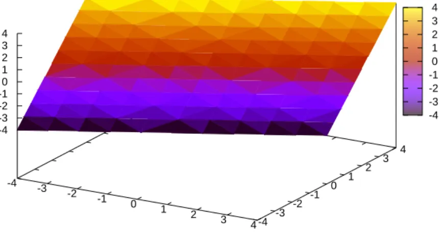
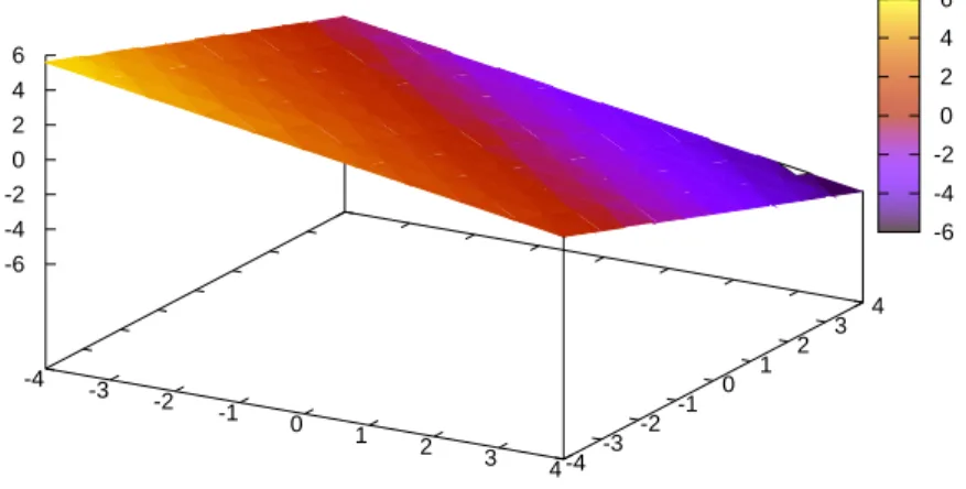
We can plot planes with implicitplot from thedraw package.

First let us define the plane with equation

3x+ 4y+ 5z = 0.

We store the equation of the plane in the variable plane1.

(%i1) plane1: 3*x + 4*y + 5*z = 0;

(%o1)

5z+ 4y+ 3x= 0 (%i2) load(draw);

(%o2)

/usr/local/share/maxima/5.19.2/share/draw/draw.lisp

(%i3) draw3d(enhanced3d = true, implicit(plane1, x,-4,4, y,-4,4, z, -6,6));

(%o3)

[gr3d (implicit)]

(9)

-4 -3 -2 -1 0 1 2 3

4 -4

-3 -2 -1 0 1 2 3 4 -6

-4 -2 0 2 4 6

-6 -4 -2 0 2 4 6

Figure 1: A plot of a plane

Let us next plot an ellipsoid with equation x²

3 +y²+z² = 3.

We plot it just like we plot the plane.

(%i4) ellips1: x^2/3 + y^2 + z^2 = 3;

(%o4)

z²+y²+x² 3 = 3

(%i5) draw3d(enhanced3d = true, implicit(ellips1, x,-3,3, y,-2,2, z, -2,2));

(%o5)

[gr3d (implicit)]

We can also use Maxima to help us find an equation of a plane based on defining vectors.

For instance, let’s find and plot the plane determined by the points A(1,1,1), B(1,2,3), and C(0,0,0).

First we define the position vectors for the three defining points.

(%i6) a: [1, 1, 1];

(%o6)

[1,1,1]

(10)

-3 -2

-1 0

1 2

3 -2

-1.5-1-0.5 0 0.5 1 1.5 2 -2

-1.5 -1 -0.5 0 0.5 1 1.5 2

-2 -1.5 -1 -0.5 0 0.5 1 1.5 2

Figure 2: A plot of an ellipsoid (%i7) b: [1, 2, 3];

(%o7)

[1,2,3]

(%i8) c: [0, 0, 0];

(%o8)

[0,0,0]

Next, we find the vectors from A to B, and A toC.

(%i9) ab: b - a;

(%o9)

[0,1,2]

(%i10) ac: c - a;

(%o10)

[−1,−1,−1]

Then, we find the normal vector to the plane. (Recall that we need the vectpackage to do cross products.)

(%i11) load(vect);

(11)

(%o11)

(%i12) n: express(ab ~ ac);

(%o12)

[1,−2,1]

Finally, we set up the defining equation of the plane, which takes the form n·r =n·r0.

(%i13) r: [x, y, z];

(%o13)

[x, y, z]

(%i14) r0: a;

(%o14)

[1,1,1]

(%i15) plane: n . r = n . r0;

(%o15)

z−2y+x= 0

The only remaining task is to make the plot. See Figure BLANK.

(%i16) draw3d(enhanced3d = true,implicit(plane,x,-4,4,y,-4,4,z,-4,4));

(%o16)

[gr3d (implicit)]

We can do more exotic plots, like cones. Let’s do a standard cone with equation x²+y² =z²

(%i17) cone: x^2 + y^2 = z^2;

(%o17)

y²+x² =z²

(%i18) draw3d(enhanced3d = true, implicit(cone, x,-1,1, y,-1,1, z,-0.5,0.5));

(12)

-4 -3

-2 -1 0 1 2 3 4 -4

-3 -2 -1 0 1 2 3 4 -4

-3 -2 -1 0 1 2 3 4

-4 -3 -2 -1 0 1 2 3 4

Figure 3: Another plot of a plane

-1

-0.5

0

0.5

1 -1 -0.5

0 0.5

1 -0.4

-0.2 0 0.2 0.4

-0.6 -0.4 -0.2 0 0.2 0.4 0.6

Figure 4: A plot of a cone

(13)

-2 -1.5 -1 -0.5 0 0.5 1 1.5

2 -2

-1.5-1-0.5 0 0.5 1 1.5 2 -1.5

-1 -0.5 0 0.5 1 1.5

-1.5 -1 -0.5 0 0.5 1 1.5

Figure 5: A plot of a hyperboloid (%o18)

[gr3d (implicit)]

See Figure BLANK. See how the center of the cone looks distorted? It is because we are plotting the cone in rectangular coordinates. We get a much better plot with spherical coordinates. More on that later.

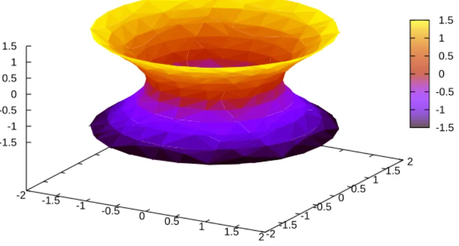
Let’s next try a hyperboloid with equation

x²+y²−z² = 1

See Figure BLANK.

(%i19) hyperboloid: x^2 + y^2 - z^2 = 1;

(%o19)

−z²+y²+x² = 1

(%i20) draw3d(enhanced3d = true, implicit(hyperboloid, x,-2,2, y,-2,2, z,-1.5,1.5));

(%o20)

[gr3d (implicit)]

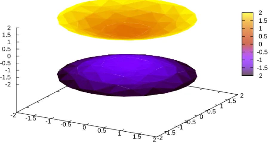
And we can do a hyperboloid of two sheets, with the equation

−x²−y²+z² = 1.

(14)

-2 -1.5 -1 -0.5 0 0.5 1 1.5

2 -2

-1.5-1-0.5 0 0.5 1 1.5 2 -2

-1.5 -1 -0.5 0 0.5 1 1.5 2

-2 -1.5 -1 -0.5 0 0.5 1 1.5 2

Figure 6: Another plot of a hyperboloid See Figure BLANK.

(%i21) hyprbld2: -x^2 - y^2 + z^2 = 1;

(%o21)

z²−y²−x² = 1

(%i22) draw3d(enhanced3d = true, implicit(hyprbld2, x,-2,2, y,-2,2, z, -2,2));

(%o22)

[gr3d (implicit)]

2.3 Vector Valued Functions

We define vector functions in Maxima just like we would any other function; the only differ- ence is that the return value is a vector.

(%i1) r(t) := [t, cos(t), sin(t)];

(%o1)

r(t) := [t,cost,sint]

Once we have the function we can plug in values of t to evaluate.

(%i2) r(1);

(15)

-1 -0.8 -0.6

-0.4 -0.2 0

0.2 0.4

0.6 0.8 1 -1-0.8-0.6-0.4-0.2 0 0.2 0.4 0.6 0.8 1 -0.8

-0.6 -0.4-0.2 0.2 0.4 0.6 0.8 0

Figure 7: A space curve in 3-d (%o2)

[1,cos 1,sin 1]

(%i3) float(%);

(%o3)

[1.0, .5403023058681398, .8414709848078965]

Now let’s try some plotting. Let’s first try a space curve of the vector function. We need the drawpackage to make this happen. Once we have it loaded, we do space curves with the parametric function inside of a draw command.

(%i4) load(draw);

(%o4)

(%i5) draw3d(parametric(cos(t), -cos(t), sin(t), t, -4, 4));

(%o5)

[gr3d (parametric)]

See Figure 1. Sometimes the line width of a space curve leaves something to be desired.

We can fix the issue with the line width argument to the draw command. See Figure 2.

(16)

Limits of vector functions operate just like limits of everything else. Notice below how to do limits from the right and left.

(%i6) limit(r(t), t, 2);

(%o6)

[2,cos 2,sin 2]

(%i7) float(%);

(%o7)

[2.0,−.4161468365471424, .9092974268256817]

(%i8) limit(r(t), t, 2, plus);

(%o8)

[2,cos 2,sin 2]

(%i9) limit(r(t), t, 3, minus);

(%o9)

[3,cos 3,sin 3]

Derivatives of vector-valued functions are, again, just like their one-valued counterparts.

(%i10) diff(r(t), t);

(%o10)

[1,−sint,cost]

We need to be careful, here. In both Maple and Maxima the return value of diff(r(t),t) is an expression, and is NOT a function (although it sure does look like one). Looks are deceptive in this case. Watch what happens if we try to use it like a function.

(%i11) wrong(t) := diff(r(t),t);

(%o11)

wrong (t) := diff (r(t), t) (%i12) wrong(1);

** error while printing error message **

~:M: second argument must be a variable; found ~M

#0: wrong(t=1)

– an error. To debug this try debugmode(true);

This is not right. The way to get around this in Maple is to do D(r(t),t), and the way to get around this in Maxima is to do the following.

(17)

(%i13) define(rp(t), diff(r(t), t));

(%o13)

rp (t) := [1,−sint,cost]

Now we get what we expect.

(%i14) float(rp(1));

(%o14)

[1.0,−.8414709848078965, .5403023058681398]

We may define the unit tangent vector T as the normalized derivative of r. We do this with the uvect function in the eigen package.

(%i15) load(eigen);

(%o15)

/usr/local/share/maxima/5.19.2/share/matrix/eigen.mac

(%i16) uvect(rp(t));

(%o16)

"

1

p(sint)²+ (cost)² + 1,− sint

p(sint)²+ (cost)²+ 1, cost

p(sint)² + (cost)²+ 1

#

(%i17) trigsimp(%);

(%o17)

1

√2,−sint

√2 ,cost

√2

(%i18) define(T(t), %);

(%o18)

T (t) :=

1

√2,−sint

√2,cost

√2

To get the unit normal vector we need to get the derivative of T and normalize.

(%i19) define(Tp(t), diff(T(t), t));

(%o19)

Tp (t) :=

0,−cost

√2 ,−sint

√2

(18)

(%i20) uvect(Tp(t));

(%o20)

"

0,− cost

p(sint)²+ (cost)²,− sint

p(sint)² + (cost)²

#

(%i21) trigsimp(%);

(%o21)

[0,−cost,−sint]

(%i22) define(N(t), %);

(%o22)

N(t) := [0,−cost,−sint]

Now we find the binormal vector, B, by calculating the cross product of T and N.

Remember to do load(vect) if you haven’t already during the session.

(%i23) load(vect);

(%o23)

/usr/local/share/maxima/5.19.2/share/vector/vect.mac (%i24) express(T(t) ~ N(t));

(%o24)

(sint)²

√2 +(cost)²

√2 ,sint

√2,−cost

√2

(%i25) trigsimp(%);

(%o25)

1

√2,sint

√2,−cost

√2

(%i26) define(B(t), %);

(%o26)

B(t) :=

1

√2,sint

√2,−cost

√2

(%i27) float(B(1));

(%o27)

[.7071067811865475, .5950098395293859,−.3820514243700898]

(19)

2.4 Arc Length and Curvature

There is no special Maxima function for the curvature but we can do it with the formulas we learned in class. Recall from the last section that r(t) =ht, cos t, sintiand

T(t) = 1

√2, −sin t

√2 , cost

√2

.

with derivative

T^′(t) =

0, −cos t

√2 , −sin t

√2

.

(%i1) r(t) := [t, cos(t), sin(t)];

(%o1)

r(t) := [t,cost,sint]

(%i2) rp(t) := [1 ,-sin(t), cos(t)];

(%o2)

rp (t) := [1,−sint,cost]

(%i3) Tp(t) := [0, -cos(t), sin(t)]/sqrt(2);

(%o3)

Tp (t) := [0,−cost,sint]

√2

(%i4) sqrt(Tp(t) . Tp(t))/sqrt(rp(t) . rp(t));

(%o4)

q(sint)²

2 + ^(cos₂^t)² p(sint)²+ (cost)²+ 1

(%i5) trigsimp(%);

(%o5)

1 2 (%i6) define(kappa(t), %);

(%o6)

κ(t) := 1 2

We have a lot of practice with derivatives, but we can integrate, too.

(%i7) integrate(r(t), t);

(20)

(%o7)

t²

2,sint,−cost

With integrals we can compute the arc length, but be warned, the arc length may only

*rarely* be calculated in closed form. More often than not the arc length can not be represented by an elementary function. We do an example for the sake of argument. We will define a simple vector function, calculate the derivative, and integrate the norm of the derivative.

(%i8) g(t) := [2 * t, 3 * sin(t), 3 * cos(t)];

(%o8)

g(t) := [2t,3 sint,3 cost]

(%i9) define(gp(t), diff(g(t), t));

(%o9)

gp (t) := [2,3 cost,−3 sint]

(%i10) integrate(trigsimp(sqrt(gp(t) . gp(t))), t, 0, 2*%pi);

(%o10)

2√ 13π

Note that we used the special notation %pi for our favorite mathematical constant. We need the same thing for Euler’s constant%e and the imaginary unit %i.

Also note that we wrapped sqrt(gp(t) . gp(t)) with trigsimp in the integrate call. As of the time of this writing, there is a bug in Maxima so that the integral is not computed correctly without the simplification. See Bug ID: 2880797 in the Maxima bug tracker.

Especially with arc lengths sometimes we need to do numerical integration instead of symbolic integration. We can do it with the romberg function.

(%i11) romberg(sqrt(gp(t) . gp(t)), t, 0, 2*%pi);

(%o11)

22.65434679827795

3 Functions of Several Variables

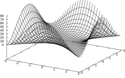
Now let’s try some multivariate functions.

(%i1) f(x,y) := (x^2 - y^2)^2;

(21)

-3 -2

-1 0

1 2

3 -3 -2

-1 0

1 2

3 0

10 20 30 40 50 60 70 80

Figure 8: A plain surface plot of a function of two variables (%o1)

f(x, y) := x²−y²₂

Let’s take a look at a plot.

(%i2) load(draw);

(%o2)

(%i3) draw3d(explicit(f(x,y), x, -3, 3, y, -3, 3));

(%o3)

[gr3d (explicit)]

See Figure BLANK.

The important part is to enclose the function with explicit(). We can get a fancier, colored plot if we put enhanced3d = trueat the beginning of the function call.

(%i4) draw3d(enhanced3d = true, explicit(f(x,y), x, -3, 3, y, -3, 3));

(%o4)

[gr3d (explicit)]

We can see level curves (also known as a contour map) of the function f with the following:

(22)

-3 -2

-1 0

1 2

3 -3 -2

-1 0

1 2

3 0

10 20 30 40 50 60 70 80

0 10 20 30 40 50 60 70 80 90

Figure 9: An enhanced surface plot of a function of two variables

(%i5) draw3d(explicit(f(x,y), x, -5, 5, y, -5, 5), contour_levels = 15,

contour = map);

(%o5)

[gr3d (explicit)]

An alternative is to use

(%i6) contour_plot(f(x,y), [x, -5, 5], [y, -5, 5] );

(%o6)

false

The contour map is a 2D plot. If we raise the contour lines up to the plot surface then the lines are more precisely called horizontal traces. Here is a plot of these.

(%i7) draw3d(enhanced3d = true,

explicit(f(x,y), x, -3, 3, y, -3, 3), contour_levels = 15,

contour = surface, surface_hide = true);

(%o7)

[gr3d (explicit)]

(23)

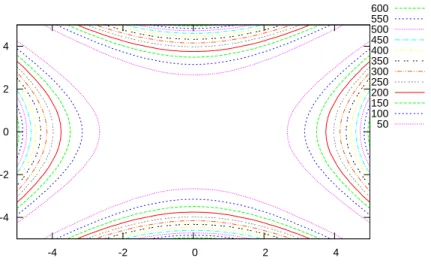
600 550 500 450 400 350 300 250 200 150 100 50

-4 -2 0 2 4

Figure 10: A contour plot, showing level curves of f.

See Figure 6. We do surfacehide = true so that we can see the traces better.

3.1 Partial Derivatives

We do partial derivatives in the natural way. For example, for the partial derivative with respect to xwe do

(%i1) diff(f(x,y), x);

(%o1)

d

d xf(x, y)

The long way to get higher order derivatives is to nest the diff calls. The second order partial derivative is

(%i2) diff(diff(f(x,y), x), x);

(%o2)

d²

d x² f(x, y) and the second partial with respect to x then y is (%i3) diff(diff(f(x,y), x), y);

(24)

80 70 60 50 40 30 20 10

-3 -2

-1 0

1 2

3 -3 -2

-1 0

1 2

3 0

10 20 30 40 50 60 70 80

0 10 20 30 40 50 60 70 80 90

Figure 11: Another form of contour plot which shows horizontal traces on f (%o3)

d²

d x d yf(x, y)

For higher order partial derivatives a quicker way is to do (%i4) G: x^7 * y^8;

(%o4)

x⁷y⁸

(%i5) diff(G, x, 1, y, 2, x, 3);

(%o5)

47040x³y⁶

The above first differentiates G with respect to x three times, then with respect to y two times, and finally with respect to xone time; that is, the arguments match the Leibnitz notation for partial derivatives.

3.2 Linear Approximation and Differentials

A function of two variables is differentiable at a point(x0, y0)when it is closely approximated by the tangent plane to the curve at(x₀, y₀). We saw in class how to find the tangent plane

(25)

at(x₀, y₀), and we also discussed how we could use the tangent plane to approximate values of f(x, y) for (x, y)near (x0, y0).

We will not bother with the tangent plane in Maxima, but we can quickly find the linear approximationLtof (which is essentially the same thing) by means of thetaylorfunction.

Let f(x, y) = e^x²sin(y) and let us find the linear approximation of f at the point (1,2).

(%i1) f(x,y) := exp(x^2) * sin(y);

(%o1)

f(x, y) := expx² siny

(%i2) taylor(f(x,y), [x,y], [1,2], 1);

(%o2)

sin 2e+ (2 sin 2e (x−1) + cos 2e (y−2)) +· · ·

The function Lis shown in the output as everything but the three dots. The ellipsis is a way to indicate that the returned expression is an approximation to the original function.

The linear approximation arguments are all self explanatory except the last. It represents the order of the Taylor series. When we find a linear approximation to a differentiable function what we are actually doing is finding a Taylor series of order 1, about the point (x0, y0).

We can get the total differential by doing diff without specifying any independent variables.

(%i3) diff(f(x,y));

(%o3)

e^x² cosydel (y) + 2x e^x² sinydel (x)

The symbols del(y) and del(x) stand for dy and dx, respectively.

3.3 Chain Rule and Implicit Differentiation

Suppose we have a function of two variables, f(x, y) = e^x² sin y.

(%i1) f(x,y) := exp(x^2) * sin(y);

(%o1)

We saw earlier what the partial derivatives of f were with respect to x and y. But suppose x and y are functions of some other variables, for instance,

(%i2) [x,y] : [s^2 * t, s * t^2];

(26)

(%o2)

s²t, s t²

Then what are the partial derivatives of f with respect to s and t? Happily for us, Maxima does the chain rule automatically.

(%i3) diff(f(x,y), s);

(%o3)

4s³t²e^s⁴^t² sin s t²

+t²e^s⁴^t² cos s t²

(%i4) diff(f(x,y), t);

(%o4)

2s⁴t e^s⁴^t² sin s t²

+ 2s t e^s⁴^t² cos s t²

That was easy. But be warned that the derivative with respect to x does not work anymore.

** error while printing error message **

~:M: second argument must be a variable; found ~M – an error. To debug this try debugmode(true);

We could fix this by using different letters, u and v:

(%i6) diff(f(u,v), u);

(%o6)

2u e^u² sinv

But that is cheating. A better way to fix it is to kill the relationship between x ands,t.

(%i7) kill(x, y);

(%o7)

done

(%o8)

2x e^x² siny

(27)

Implicit differentiation is relatively easy, given what we have already done. For example, let’s find the first partial derivatives of z when xyz+x²y³z⁴ =x+xz.

(%i9) F: x*y*z + x^2*y^3*z^4 - x - x*z;

(%o9)

x²y³z⁴+x y z−x z−x

(%i10) Fx: diff(F, x);

(%o10)

2x y³z⁴+y z−z−1

(%i11) Fy: diff(F, y);

(%o11)

3x²y²z⁴+x z

(%i12) Fz: diff(F, z);

(%o12)

4x²y³z³+x y−x

(%i13) [-Fx/Fy, -Fy/Fz];

(%o13)

−2x y³z⁴−y z+z+ 1

3x²y²z⁴+x z , −3x²y²z⁴−x z 4x²y³z³ +x y−x

3.4 Directional Derivatives and the Gradient

Remember to doload(vect) if you haven’t already during the session. By default Maxima assumes that the coordinate system is rectangular (cartesian) in the variables x,y, andz. If you do not want that then you need to change it by means of the scalefactorscommand.

Given the function of two variables, f(x, y) = e^x² siny.

(%i1) f(x,y) := exp(x^2) * sin(y);

(%o1)

We change to the correct coordinate system.

(%i2) load(vect);

(28)

(%o2)

(%i3) scalefactors([x,y]);

(%o3)

done

Next we find the gradient.

(%i4) gdf: grad(f(x,y));

(%o4)

grad

e^x² siny

(%i5) ev(express(gdf), diff);

(%o5)

h2x e^x² siny, e^x² cosyi

(%i6) define(gdf(x,y), %);

(%o6)

gdf (x, y) :=h

2x e^x² siny, e^x² cosyi

The directional derivative of f at the point(1,2)in the direction of the vectorv=h3,4i is

(%i7) v: [3,4];

(%o7)

[3,4]

(%i8) (gdf(1,2) . v)/sqrt(v . v);

(%o8)

6e sin 2 + 4e cos 2 5

(%i9) ev(%, diff);

(%o9)

6e sin 2 + 4e cos 2 5

(%i10) float(%);

(29)

(%o10)

2.061108499400332

We know from our theory that the directional derivative is maximized when v points in the direction of the gradient, and the maximum value is the length of the gradient vector.

Let’s see just how big that is.

(%i11) sqrt(gdf(1,2) . gdf(1,2));

(%o11)

p4e² (sin 2)²+e² (cos 2)²

(%i12) float(ev(%, diff));

(%o12)

5.071228088168654

3.5 Optimization and Local Extrema

To find critical points we need to solve the system of equations fx = 0 and fy = 0. Let f(x, y) = 2x⁴+ 2y⁴−8xy.

(%i1) f(x,y) := 2 * x^4 + 2 * y^4 - 8 * x * y;

(%o1)

f(x, y) := 2x⁴+ 2y⁴+ (−8) x y

Let’s take a look at a plot of f. (%i2) load(draw);

(%o2)

(%i3) draw3d(enhanced3d = true, explicit(f(x,y), x, -2, 2, y, -2, 2));

(%o3)

[gr3d (explicit)]

See Figure BLANK.

Now let’s take a look at a contour plot of f. We do it just like the plot of the surface, except we use the argument contour = map.

(30)

-2 -1.5 -1 -0.5 0 0.5 1 1.5

2 -2

-1.5-1-0.5 0 0.5 1 1.5 2 0

10 20 30 40 50 60 70 80 90

-10 0 10 20 30 40 50 60 70 80 90 100

Figure 12: A surface plot of f

(%i4) draw3d(explicit(f(x,y), x, -2, 2, y, -2, 2), contour = map);

(%o4)

[gr3d (explicit)]

See Figure BLANK.

Now let’s find the first order partial derivatives off, set them equal to zero, and solve for values of(x, y). We do this with thesolvefunction, which assumes that the expressions are set equal to zero by default. Keep in mind that solve finds all real and complex solutions;

we only care about the real valued solutions, however, and will ignore the rest.

(%i5) fx : diff(f(x,y), x);

(%o5)

8x³−8y

(%i6) fy : diff(f(x,y), y);

(%o6)

8y³−8x (%i7) solve([fx,fy], [x,y]);

(31)

90 85 80 75 70 65 60 55 50 45 40 35 30 25 20 15 10 5 0

-2 -1.5 -1 -0.5 0 0.5 1 1.5 2

Figure 13: The level curves of f which suggest two extrema and a saddle point (%o7)

hhx= (−1)¹⁴ i, y =−(−1)³⁴ ii ,h

x=−(−1)¹⁴, y =−(−1)³⁴i ,h

x=

−(−1)¹⁴ i, y = (−1)³⁴ ii ,h

x= (−1)¹⁴, y = (−1)³⁴i ,[x=

−i, y =i],[x=i, y =−i],[x=−1, y =−1],[x= 1, y = 1],[x= 0, y = 0]i Critical points are at(0,0),(1,1), and(−1,−1). (Note that both partial derivatives exist everywhere.) We need to see what the Hessian says at those locations.

(%i8) H: hessian(f(x,y), [x,y]);

(%o8)

24x² −8

−8 24y²

(%i9) determinant(H);

(%o9)

576x²y²−64

We do the Second Derivative Test by plugging in the above three points into fxx and det(H). (Of course we can do it mentally but let’s try it with Maxima.) A quick way to plug numbers into expressions is with the subst function.

(32)

(%i10) subst([x = -1, y = -1], diff(fx, x));

(%o10)

24

(%i11) subst([x = -1, y = -1], determinant(H));

(%o11)

512

From the above we conclude that (−1,−1)is a local minimum of f, and the value is (%i12) f(-1,-1);

(%o12)

−4

Doing the same for (0,0) and (1,1) shows that (0,0) is a saddle point and (1,1) is also a local minimum (we know this already by symmetry).

3.6 Lagrange Multipliers

Find the extreme values of the function f(x, y) = 2x²+y² on the circlex²+y² = 1.

(%i1) f(x,y) := 2 * x^2 + y^2;

(%o1)

f(x, y) := 2x²+y²

(%i2) g: x^2 + y^2;

(%o2)

y²+x²

We set up the system of equations grad(f) = h * grad(g), g = 1. (We do not use

"lambda" because that name is already reserved for an existing function in Maxima.) (%i3) eq1: diff(f(x,y), x) = h * diff(g, x);

(%o3)

4x= 2h x (%i4) eq2: diff(f(x,y), y) = h * diff(g, y);

(%o4)

2y = 2h y (%i5) eq3: g = 1;

(33)

(%o5)

y²+x² = 1

Now we solve the system for x,y, andh.

(%i6) solve([eq1, eq2, eq3], [x, y, h]);

(%o6)

[[x= 1, y = 0, h= 2],[x=−1, y = 0, h= 2],[x= 0, y =−1, h= 1],[x= 0, y = 1, h= 1]]

We see that the extreme values lie among (1,0), (−1,0), (0,−1), (0,1).

(%i7) [f(1,0), f(-1,0), f(0,-1), f(0,1)];

(%o7)

[2,2,1,1]

So the minima occur at (1,0)and (−1,0); the maxima occur at (0,−1) and (0,1).

4 Multiple Integration

4.1 Double Integrals

We can iterate integrate calls. For example, suppose we wanted to calculate Z Z

x³−3xy

dydx.

(%i1) f(x,y) := x^3 - 3*x*y;

(%o1)

f(x, y) :=x³−3x y

(%i2) integrate(integrate(f(x,y), y), x);

(%o2)

x⁴y

4 −3x²y² 4

Maxima does not provide arbitrary constants of integration; the user must remember them. It is easy to do definite integration, for example, we could do

Z 1Z 2−x

√ x³−3xy

dydx.

(34)

with

(%i3) integrate(integrate(f(x,y), y, x^1/2, 2 - x), x, 0, 1);

(%o3)

−173 160

4.2 Integration in Polar Coordinates

We can integrate in polar coordinates in the obvious way. We simply make the substitution x = rcos(theta) and y = rsin(theta), then don’t forget to multiply the integrand by r.

(%i1) f(x,y) := x^2 + y^2;

(%o1)

f(x, y) :=x²+y²

(%i2) [x,y]: [r * cos(theta), r * sin(theta)];

(%o2)

[r cosϑ, r sinϑ]

(%i3) integrate(integrate(f(x,y) * r, r, 0, 2*cos(theta)), theta, -%pi/2,

%pi/2);

(%o3)

3π 2

4.3 Triple Integrals

Triple integrals are done just like double integrals: by nestedintegrate calls.

Let’s do

Z 1

0

Z ₋x

0

Z x+y

0

x²yz dzdydx.

(%i1) integrate(integrate(integrate(x^2*y*z,z,0,x+y),y,0,-x),x,0,1);

(%o1)

1 168

(35)

4.4 Integrals in Cylindrical and Spherical Coordinates

These integrals are computed just like ordinary triple integrals except we multiply the integrand by r (in cylindrical coordinates) orρ²sin(φ) (in spherical coordinates). See the next section for a more general way of doing this. It is sometimes useful to use plots to decide how to represent the region of integration.

Let’s do an integral in cylindrical coordinates.

Z 2

−2

Z

√4−x²

0

Z 3

0

yz dzdydx.

Note that r goes from 0 to 2 and θ goes from 0 to π.

(%i1) f(x,y,z) := y*z;

(%o1)

f(x, y, z) :=y z

(%i2) [x,y,z] : [r*cos(theta), r*sin(theta), z];

(%o2)

[r cosϑ, r sinϑ, z]

(%i3) integrate(integrate(integrate(f(x,y,z)*r, z,0,3), r,0,2), theta,0,%pi);

(%o3)

24

Now let’s do an integral in spherical coordinates.

Z 1

−1

Z ^√1−x²

0

Z √

1−x²−y² 0

xz dzdydx.

Note that ρ goes from 0 to 1,θ goes from 0 to π, and φ goes from 0 to π/2.

(%i4) kill(f,x,y,z);

(%o4)

done

(%i5) f(x,y,z) := x*z;

(%o5)

f(x, y, z) :=x z

(%i6) [x,y,z] : [rho*sin(phi)*cos(theta), rho*sin(phi)*sin(theta), rho*cos(theta)];

(%o6)

[sinϕ ρcosϑ,sinϕ ρsinϑ, ρ cosϑ]

(36)

(%i7) integrate(integrate(integrate(f(x,y,z)*rho^2*sin(phi),rho,0,1),theta,0,%pi), phi,0,%pi/2);

(%o7)

π² 40

4.5 Change of Variables

For more general transformations x = x(u, v) and y = y(u, v) we can use the jacobian function in the linearalgebra package, which is loaded by default. Let f(x, y) = x+y, and we will calculate

Z Z

R

(x+y) dA.

(%i1) f(x,y) := x + y;

(%o1)

f(x, y) :=x+y

Let’s make the transformation x=u³−v⁴ and y= 5uv.

(%i2) [x,y]: [u^3 - v^4, 5 * u * v];

(%o2)

u³ −v⁴,5u v

We need the Jacobian:

(%i3) J: jacobian([x,y], [u,v]);

(%o3)

3u² −4v³ 5v 5u

(%i4) J: determinant(J);

(%o4)

20v⁴+ 15u³

We were lucky in this example because the Jacobian is positive as long asuis positive (or just not terribly negative). If this had not happened then we would need to be careful about the sign of J, which in principle could be a problem because Maxima does not integrate

(37)

absolute value. Nevertheless, we finish up with the integration. It takes the form (we will make up random limits of integration, but in a given problem we would need to determine these)

Z 4

3

Z 2

1

f(x(u, v), y(u, v))

∂(x, y)

∂(u, v)

dudv.

(%i5) integrate(integrate(f(x,y) * J, u,1,2), v,3,4);

(%o5)

−113349305 252

5 Vector Calculus

5.1 Vector Fields

A vector field is a vector function defined on a subset of R³ (or R²) that assigns a vector (of the same dimension) with each point in the set.

Two-dimensional

A two dimensional vector field associates a two-dimensional vector with each point in the plane (or a subset thereof). We may use thedrawpackage to plot vector fields with Maxima.

load ( draw );

Let us plot the 2D vector field F(x, y) =hcos y, xi.

The important parts of the following code are the first line where we specify that plotting should be done from-6to6and in thevf2dline where we specify function values[cos(y),x]

in the second list. The division by 6 in that same line is just to make the arrows smaller so that they may more easily be seen. The rest of the code is boilerplate and may be copied/pasted verbatim.

coord : setify ( makelist (k ,k , -4 ,4));

points2d : listify ( c a r t e s i a n _ p r o d u c t ( coord , coord ));

vf2d (x , y ):= vector ([ x , y ] ,[ cos ( y ) , x ]/6);

vect2 : makelist ( vf2d ( k [1] , k [2]) , k , points2d );

apply ( draw2d , append ([ color = blue ] , vect2 ));

See Figure BLANK.

Gradient vector fields

The gradient vector ∇f defines a vector field on the domain of f. We can plot this vector field in two ways: with the draw package, or with the ploteq function.

First we need a gradient function. Let’s start with f(x, y) = x²−y². Then, of course,

∇f =h2x, −2yi.

(38)

-4 -3 -2 -1 0 1 2 3 4

Figure 14: A plot of the vector field F(x, y) =hcos y, xi kill (f , x , y , gdf );

f (x , y ) := x ^2 - y ^2;

s c a l e f a c t o r s ([ x , y ]);

gdf (x , y ) := grad ( f (x , y ));

ev ( express ( gdf (x , y )) , diff );

define ( gdf (x , y ) , %);

Next we make the plot. (We have omitted the first few lines because we will use the same values from the last example. However, these lines should not ordinarily be skipped).

vf2d (x , y ) := vector ([ x , y ] , gdf (x , y )/8);

vect2 : makelist ( vf2d ( k [1] , k [2]) , k , points2d );

apply ( draw2d , append ([ h e a d _ l e n g t h =0.1 , color = blue ] , ve ct2 ));

Alternatively, we can do it in one line with theploteqfunction as long as we remember to put a minus sign in front of the original function (ploteqplots vectors that are the opposite of gradient vectors).

ploteq ( -( x ^2+ y ^2) ,[ x , y ] ,[ x , -4 ,4] ,[ y , -4 ,4] ,[ vectors ," blue "]);

Three-dimensional

This is almost identical to the 2D case, except that we need to account forz in the code and use draw3d instead of draw2d.

Note that with 3d plots the graph can be dynamically moved around with the mouse to look from different angles. Also note that the arrows in a vector field plot are often times difficult to see because of their length. I usually scale them down to see the relationships better.

(39)

-4 -3 -2 -1 0 1 2 3 4

-4 -2 0 2 4

Figure 15: The gradient vector field ∇f for the function f(x, y) = x²−y² Let’s plot the vector field

F(x, y, z) =hz, x, yi. coord : setify ( makelist (k ,k , -2 ,2));

points3d : listify ( c a r t e s i a n _ p r o d u c t ( coord , coord , coor d ));

vf3d (x ,y , z ):= vector ([ x ,y , z ] ,[ z ,x , y ]/8);

vect3 : makelist ( vf3d ( k [1] , k [2] , k [3]) , k , points3d );

apply ( draw3d , append ([ color = blue ] , vect3 ));

See Figure BLANK.

5.2 Line Integrals

We are given a smooth space curveC defined by the parametric equationsx=x(t),y=y(t), z =z(t), for a≤t ≤b, and a function f which is defined on C. Sometimes we work with a vector functionr instead of the parametric equations:

r(t) =hx(t), y(t), z(t)i, for a≤t≤b.

With respect to arc length These integrals are of the form

Z

C

f(x, y, z) ds which can be reparameterized as

Z b

f(x(t), y(t), z(t)) s

dx dt

2

+ dy

dt 2

+ dz

dt 2

dt

(40)

-2 -1.5 -1 -0.5 0 0.5 1 1.5 2 -2-1.5-1-0.5 0 0.5 1 1.5 2 -2

-1.5 -1 -0.5 0 0.5 1 1.5 2

Figure 16: A plot of the vector field F(x, y, z) =hz, x, yi or more compactly as

Z b

a

f(r(t)) |r^′(t)|dt.

For example, let’s start with f(x, y) = x² +y². We will integrate along the curve C parameterized byhcos t, sin 2tifor 0≤t≤1.

(%i1) f(x,y) := x^2 + y^2;

(%o1)

f(x, y) :=x²+y²

(%i2) [x,y]: [cos(t), sin(2*t)];

(%o2)

[cost,sin (2t)]

(%i3) rp: diff([x,y], t);

(%o3)

[−sint,2 cos (2t)]

(%i4) romberg(f(x,y)*sqrt(rp . rp), t, 0, 1);

(%o4)

1.635879048260743

(41)

Of vector fields

Here we are trying to compute integrals of the form Z

C

F·dr = Z

C

F(r(t)) · r^′(t) dt,

alternately written Z

C

P dx+Qdy+Rdz, whereF =Pi+Qj+Rk.

Let’s work with the vector field F(x, y, z) = h−xy³, xz, yz²i. We will integrate along the curve C parameterized byht², t³, t⁴i for 0≤t ≤1.

(%i5) F(x,y,z) := [-x*y^3, x*z, y*z^2];

(%o5)

F (x, y, z) :=

(−x) y³, x z, y z²

(%i6) [x,y,z]: [t^2, t^3, t^4];

(%o6)

t², t³, t⁴

(%i7) romberg(F(x,y,z) . diff([x,y,z], t), t, 0, 1);

(%o7)

.4461538461603605

5.3 Conservative Vector Fields and Finding Scalar Potentials

We know from theory that a vector field F is conservative if there exists a functionf such that F=∇f. Further, we know that fields defined on suitably nice regions are conservative if they are irrotational.

We can check whether a field is conservative with thecurlfunction in the vectpackage.

For example, let’s check the field F(x, y) = (4x³−5y²)i+ (5y³−3x)j.

(%i1) F(x,y) := [4*x^3 - 5*y^2, 5*y^3 - 3*x];

(%o1)

F (x, y) :=

4x³−5y²,5y³−3x

(%i2) load(vect);

(%o2)

/usr/local/share/maxima/5.19.2/share/vector/vect.mac (%i3) scalefactors([x,y]);

(42)

(%o3)

done

(%i4) curl(F(x,y));

(%o4)

curl

4x³−5y²,5y³−3x

(%i5) express(%);

(%o5)

d

d x 5y³−3x

− d

d y 4x³−5y² (%i6) ev(%, diff);

(%o6)

10y−3

Since the curl is not zero, the field is not conservative. How about F(x, y) = (x³+ 5y)i+ (5y³+ 5x)j?

(%i7) F(x,y) := [x^3 + 5*y, 5*y^3 + 5*x];

(%o7)

F(x, y) :=

x³+ 5y,5y³ + 5x

(%i8) ev(express(curl(F(x,y))), diff);

(%o8)

0

Since the curl is zero, this field is conservative. So the function f satisfying F = ∇f exists. We can find the scalar potential f in Maxima with the potential function (also in the vect package).

Note, however, that because of a bug in Maxima at the time of this writing we need to do a little fancy footwork. We cannot use the letter x in the function call; instead we will change it to another letter. When we do that, we must follow it by a call toscalefactors.

(%i9) F(u,v) := [u^3 + 5*v, 5*v^3 + 5*u];

(%o9)

F(u, v) :=

u³+ 5v,5v³+ 5u (%i10) scalefactors([u,v]);

(43)

(%o10)

done (%i11) potential(F(u,v));

(%o11)

5v⁴+ 20u v+u⁴ 4

We can easily check thatf(x, y) = (5x⁴+20xy+y⁴)/4satisfiesF=∇f. The fundamental theorem for line integrals now allows us to compute line integrals that look like

Z

C

F·dr = Z

C∇f ·dr,

which simplifies to f(r(b))−f(r(a)). So, for instance, for a curveC with initial point (0,1) and terminal point (2,3)we have

Z

C

F·dr = Z

C

(x³+ 5y)i+ (5y³+ 5x)j

·dr

to be equal to (using the result frompotential, above) (%i12) define(f(u,v), %);

(%o12)

f(u, v) := 5v⁴+ 20u v+u⁴ 4

(%i13) f(2,3) - f(0,1);

(%o13)

134

All of the above can be done in three dimensions, too. We need only to doscalefactors([x,y,z]) and scalefactors([u,v,w]), when appropriate.

6 Miscellaneous

6.1 Saving your plots

In most Microsoft Windowsr applications, you can save a plot either with a direct option in a File menu, or if nothing else, by right-clicking on the plot and selecting "Copy". Un- fortunately, with the plots described in this document (and on Linux, at least), this is not possible. Instead, the user must separately send the plot to a file.

In the drawpackage plots can be saved with the terminal argument. The following are a couple of examples of what this looks like, and see the documentation for terminal for more details and options. For a standard 2d plot you can usually get by with something like this:

(44)

draw3d ( e n h a n c e d 3 d = true ,

implicit ( plane1 , x , -4 ,4 , y , -4 ,4 , z , -6 ,6) , terminal = eps_color , file_name =" plot ");

But for the more complicated vector field plots you need something like this:

apply ( draw3d ,

append ([ color = blue ,

terminal = eps_color , file_name =" plot "] , vect3 ));

6.2 Saving your Maxima commands

Once you type a bunch of commands into Maxima you will often want to save those commands into a file to be opened and used again later. The following command will pick out all of the Maxima commands from the session and save them into a text file that can be opened later with any text editor.

Note that only commands since the last kill(all) statement will be saved.

stringout (" n a m e o f f i l e . txt " , input , f i l e _ o u t p u t _ a p p e n d = true );

(45)

7 GNU Free Documentation License

Version 1.3, 3 November 2008

Everyone is permitted to copy and distribute verbatim copies of this license document, but changing it is not allowed.

0. PREAMBLE

The purpose of this License is to make a manual, textbook, or other functional and useful document "free" in the sense of freedom: to assure everyone the effective freedom to copy and redistribute it, with or without modifying it, either commercially or noncommercially.

Secondarily, this License preserves for the author and publisher a way to get credit for their work, while not being considered responsible for modifications made by others.

This License is a kind of "copyleft", which means that derivative works of the document must themselves be free in the same sense. It complements the GNU General Public License, which is a copyleft license designed for free software.

We have designed this License in order to use it for manuals for free software, because free software needs free documentation: a free program should come with manuals providing the same freedoms that the software does. But this License is not limited to software manuals; it can be used for any textual work, regardless of subject matter or whether it is published as a printed book. We recommend this License principally for works whose purpose is instruction or reference.

1. APPLICABILITY AND DEFINITIONS

This License applies to any manual or other work, in any medium, that contains a notice placed by the copyright holder saying it can be distributed under the terms of this License.

Such a notice grants a world-wide, royalty-free license, unlimited in duration, to use that work under the conditions stated herein. The "Document", below, refers to any such manual or work. Any member of the public is a licensee, and is addressed as "you". You accept the license if you copy, modify or distribute the work in a way requiring permission under copyright law.

A "Modified Version" of the Document means any work containing the Document or a portion of it, either copied verbatim, or with modifications and/or translated into another language.

A "Secondary Section" is a named appendix or a front-matter section of the Document that deals exclusively with the relationship of the publishers or authors of the Document to the Document’s overall subject (or to related matters) and contains nothing that could fall directly within that overall subject. (Thus, if the Document is in part a textbook of mathematics, a Secondary Section may not explain any mathematics.) The relationship could be a matter of historical connection with the subject or with related matters, or of legal, commercial, philosophical, ethical or political position regarding them.

(46)

The "Invariant Sections" are certain Secondary Sections whose titles are designated, as being those of Invariant Sections, in the notice that says that the Document is released under this License. If a section does not fit the above definition of Secondary then it is not allowed to be designated as Invariant. The Document may contain zero Invariant Sections. If the Document does not identify any Invariant Sections then there are none.

The "Cover Texts" are certain short passages of text that are listed, as Front-Cover Texts or Back-Cover Texts, in the notice that says that the Document is released under this License. A Front-Cover Text may be at most 5 words, and a Back-Cover Text may be at most 25 words.

A "Transparent" copy of the Document means a machine-readable copy, represented in a format whose specification is available to the general public, that is suitable for revising the document straightforwardly with generic text editors or (for images composed of pixels) generic paint programs or (for drawings) some widely available drawing editor, and that is suitable for input to text formatters or for automatic translation to a variety of formats suitable for input to text formatters. A copy made in an otherwise Transparent file format whose markup, or absence of markup, has been arranged to thwart or discourage subsequent modification by readers is not Transparent. An image format is not Transparent if used for any substantial amount of text. A copy that is not "Transparent" is called "Opaque".

Examples of suitable formats for Transparent copies include plain ASCII without markup, Texinfo input format, L^ATEX input format, SGML or XML using a publicly available DTD, and standard-conforming simple HTML, PostScript or PDF designed for human modification. Examples of transparent image formats include PNG, XCF and JPG. Opaque formats include proprietary formats that can be read and edited only by proprietary word processors, SGML or XML for which the DTD and/or processing tools are not generally available, and the machine-generated HTML, PostScript or PDF produced by some word processors for output purposes only.

The "Title Page" means, for a printed book, the title page itself, plus such following pages as are needed to hold, legibly, the material this License requires to appear in the title page. For works in formats which do not have any title page as such, "Title Page" means the text near the most prominent appearance of the work’s title, preceding the beginning of the body of the text.

The "publisher" means any person or entity that distributes copies of the Document to the public.

A section "Entitled XYZ" means a named subunit of the Document whose title either is precisely XYZ or contains XYZ in parentheses following text that translates XYZ in another language. (Here XYZ stands for a specific section name mentioned below, such as "Acknowledgements", "Dedications", "Endorsements", or "History".) To "Preserve the Title" of such a section when you modify the Document means that it remains a section

"Entitled XYZ" according to this definition.

The Document may include Warranty Disclaimers next to the notice which states that this License applies to the Document. These Warranty Disclaimers are considered to be included by reference in this License, but only as regards disclaiming warranties: any other implication that these Warranty Disclaimers may have is void and has no effect on the meaning of this License.

(47)

2. VERBATIM COPYING

You may copy and distribute the Document in any medium, either commercially or noncommercially, provided that this License, the copyright notices, and the license notice saying this License applies to the Document are reproduced in all copies, and that you add no other conditions whatsoever to those of this License. You may not use technical measures to obstruct or control the reading or further copying of the copies you make or distribute.

However, you may accept compensation in exchange for copies. If you distribute a large enough number of copies you must also follow the conditions in section 3.

You may also lend copies, under the same conditions stated above, and you may publicly display copies.

3. COPYING IN QUANTITY

If you publish printed copies (or copies in media that commonly have printed covers) of the Document, numbering more than 100, and the Document’s license notice requires Cover Texts, you must enclose the copies in covers that carry, clearly and legibly, all these Cover Texts: Front-Cover Texts on the front cover, and Back-Cover Texts on the back cover. Both covers must also clearly and legibly identify you as the publisher of these copies. The front cover must present the full title with all words of the title equally prominent and visible.

You may add other material on the covers in addition. Copying with changes limited to the covers, as long as they preserve the title of the Document and satisfy these conditions, can be treated as verbatim copying in other respects.

If the required texts for either cover are too voluminous to fit legibly, you should put the first ones listed (as many as fit reasonably) on the actual cover, and continue the rest onto adjacent pages.

If you publish or distribute Opaque copies of the Document numbering more than 100, you must either include a machine-readable Transparent copy along with each Opaque copy, or state in or with each Opaque copy a computer-network location from which the general network-using public has access to download using public-standard network protocols a com- plete Transparent copy of the Document, free of added material. If you use the latter option, you must take reasonably prudent steps, when you begin distribution of Opaque copies in quantity, to ensure that this Transparent copy will remain thus accessible at the stated location until at least one year after the last time you distribute an Opaque copy (directly or through your agents or retailers) of that edition to the public.

It is requested, but not required, that you contact the authors of the Document well before redistributing any large number of copies, to give them a chance to provide you with an updated version of the Document.

4. MODIFICATIONS

You may copy and distribute a Modified Version of the Document under the conditions of sections 2 and 3 above, provided that you release the Modified Version under precisely this License, with the Modified Version filling the role of the Document, thus licensing distribution