High Frequency VLBI Studies of Sagittarius A* and NRAO 530

High Frequency VLBI Studies of Sagittarius A*

and NRAO 530

Inaugural-Dissertation zur

Erlangung des Doktorgrades

der Mathematisch-Naturwissenschaftlichen Fakult¨at der Universit¨at zu K¨oln

vorgelegt von

Ru-Sen Lu aus Hebei, China

K¨oln 2010

Berichterstatter:

1.Gutachter: Prof. Dr. J. Anton Zensus

2.Gutachter: Prof. Dr. Andreas Eckart

Tag der m¨undlichen Pr¨ufung: 13.07.2010

To my parents and the rest of my familly

Abstract

Compact radio sources (Kellermann & Pauliny-Toth 1981) are widely accepted to be associated with supermassive black holes at the centers of active galaxies. Very long baseline interferometry (VLBI) observations at short millimeter wavelengths offer the unique advantage to look “deeper” into the central core regions. In this thesis we study two compact radio sources (Sagittarius A* and NRAO 530) with high frequency VLBI techniques.

As a starting point, we give in Chapter 1 a general introduction to observational properties of Active galactic nuclei (AGNs) and a theoretical basis. In Chapter 2, the compact radio source at the center of the Milky Way, Sagittarius A*, is reviewed. In Chapter 3, the technical basis of VLBI is outlined and then the difficulties of VLBI (and therefore the ways to improve) at short millimeter wavelengths are discussed.

Due to its proximity, Sagittarius A* has the largest apparent event horizon of any black hole candidate and therefore it provides a unique opportunity for testing the SMBH paradigm. However, direct imaging of the nucleus is only accessible at short millimeter wavelengths due to the scatter broadening. In Chapter 4, we present results of an inter-day VLBI monitoring of Sagittarius A* at wavelengths of 13, 7, and 3 mm during a global observing campaign in 2007. We measure the flux density and source structure and study their variability on daily time scales.

In addition to the VLBI monitoring of the Galactic Center, we present in Chapter 5 results of multi-epoch multi-frequency VLBI observations of the blazar NRAO 530.

NRAO 530 is an optically violent variable (OVV) source and was observed as a VLBI calibrator in our observations of Sagittarius A*. We investigate the spectral properties of jet components, their frequency-dependent position shifts, and variability of flux density and structure on daily time scales. Analysis of archival data over the last ten years allows us to study the detailed jet kinematics.

Finally, a summary and future outlook is given in Chapter 6.

Zusammenfassung

Nach g¨angigem Verst¨andnis befinden sich in den Zentren aktiver Galaxienkerne große, sogenannte super-massive schwarze L¨ocher. Diese aktiven Galaxienkerne manifestieren sich als kompakte Radioquellen am Himmel. Mittels der Methode der interkontinen- talen radiointerferometrischen Beobachtung (VLBI: Very Long Baseline Interferometry) bei kurzen Millimeter-Wellen¨angen, ergibt sich die einzigartige M¨oglichkeit diese Zentralregionen mit h¨ochster Winkelaufl¨osung zu untersuchen. In dieser Doktorarbeit werden die Ergebnisse einer interferometrischen VLBI-Untersuchung von zwei beson- ders prominenten kompakten Radioquellen mittels der Methode von Millimeter-VLBI vorgestellt. Bei diesen beiden Quellen handelt es sich um die Zentralquelle im Galak- tischen Zentrum (Sagittarius A, Sgr A*) und um den entfernten Quasar NRAO530.

Im einleitenden Kapitel 1 dieser Arbeit wird zuerst eine allgemeine und zusammen- fassende Darstellung der Aktiven Galaxienkerne (AGK, engl. AGN), und der sie beschreibenden zu Grunde liegenden theoretischen Modelle gegeben. Im zweiten Kapitel wird die kompakte Radioquellen Sgr A* im galaktischen Zentrum und der mo- mentane Stand der wissenschaftlichen Forschung hierzu, in einer allgemeinen ¨ Ubersicht zusammengefaßt. Im Kapitel 3 werden die technischen Grundlagen und die technis- chen Grenzen von VLBI-Beobachtungen bei Millimeter-Wellenl¨angen dargestellt und diskutiert.

Auf Grund der relativ geringen Entfernung zur Erde, hat Sagittarius A * den gr¨oßten

scheinbaren Ereignishorizont-Durchmesser aller bekannten Schwarz-Loch Kandidaten,

und erlaubt somit auf einmalige Weise das Schwarz-Loch Paradigma eines (aktiven)

Galaxienkernes durch direkte Beobachtungen zu testen. Bedingt durch die Bildver-

schmierung bei langen Radiowellen durch interstellare Szintillation, ist eine direkte

Kartierung des Kerns und der unmittelbaren Umgebung des Schwarzen Loches nur

bei kurzen Millimeter-Wellenl¨angen und mit VLBI m¨oglich. In Kapitel 4 dieser Arbeit

pr¨asentiere ich die Resultate einer neuen VLBI-Beobachtungskampagne von 10 Tagen

Dauer, die Teil einer umfassenderen multi-spektralen Messkampagne auf Sgr A* im

Mai 2007 war. Die VLBI Beobachtungen wurden bei drei Wellenl¨angen (13 mm, 7 mm, und 3 mm) durchgef¨uhrt und durch Einzelteleskop-Messungen erg¨anzt. Ziel dieser Beobachtungen war das Erfassen m¨oglicher Flussdichtevariabilit¨at und die Suche nach Variationen der Quellstruktur mit hoher zeitlicher Aufl¨osung auf einer Skala von Tagen.

Erg¨anzend zum VLBI-Monitoring von Sgr A*, zeige und diskutiere ich in Kapitel 5 dieser Arbeit die Ergebnisse der 3-Frequenz-VLBI Beobachtungen des optisch stark variablen Quasars NRAO 530 (ein OVV Blazar). Diese kompakte extragalaktische Ra- dioquelle wurde als VLBI Kalibrator und System-Test Quelle in den oben beschriebe- nen VLBI Beobachtungen von Sgr A* mitbeobachtet. Die Daten erlauben eine de- tailierte Kartierung des Jets von NRAO530, die Untersuchung der spektralen Eigen- schaften der Jet-Komponenten, die Messung einer frequenzabh¨angigen Positionsver- schiebung, sowie die Charakterisierung der Flussdichte- und Strukturvariabilit¨at auf einer Zeitskala von 1-10 Tagen. Erg¨anzt werden die hier vorgestellten Millimeter- VLBI Beobachtungen durch eine umfassende Analyse vorliegender Archiv-VLBI- Daten aus den vergangenen 10 Jahren. Damit ist ein detailiertes Studium der Jet- Kinematik ¨uber diesen Zeitraum m¨oglich.

Im letzen Kapitel (Kap. 6) fasse ich die Ergebnisse der vorangegangenen Kapitel

nochmals zusammen und gebe einen Ausblick auf die m¨ogliche zuk¨unftige Entwick-

lung, besonders in Hinblick auf mm-VLBI bei noch k¨urzeren Wellenl¨angen.

Acknowledgements

In the beginning, I would like to thank the directors of the Max-Planck-Institut f¨ur Radioastronomie who supported me through the International Max Planck Research School (IMPRS) for Astronomy and Astrophysics. I am gratefull to Prof. Dr. Anton Zensus and Prof. Dr. Andreas Eckart for being the members of my examination board and for their support. In particular, I would like to thank Prof. Dr. Anton Zensus for giving me the opportunity to do this work in the VLBI group of the MPIfR and Prof. Dr. Endreas Eckart for his support and for providing me data of the May 2007 observing campaign.

I wish to express my deep gratitude to my supervisor Dr. Thomas Krichbaum.

Thomas never got tired of giving me the advice I need to finish this work. With out his inspiring guidance, invaluable discussions, and encouragement, this study would not have been able to be fulfilled.

I will forever be grateful to my supervisor at Shanghai Astronomical Observatory, Professor Zhi-Qiang, Shen, who introduced me to astrophysical research. I thank him for his direction, dedication and encouragement through all these years.

I would also like to extend my heartfelt thanks to two other members of my IMPRS thesis committee, Dr. Arno Witzel, and Dr. Andreas Brunthaler for their invaluable advice and suggestions.

I would like to thank the various members of the VLBI group, both past and present, for their friendship and assistance. I am grateful to Dr. Richard Porcas, Priv.

Doz. Dr. Silke Britzen for their help in preparing talks and the help in several other ways. I thank Dr. David Graham, Dr. Tuomas Savolainen, Dr. Andrei Lobanov, Dr.

Yuri Kovalev, Dr. Alexander Pushkarev and Dr. Alan Roy for their help in my data reduction and sharing their knowledge. I am gratefull to Prof. Dr. Eduardo Ros for his support, humor and for the calling of Chinese VLBI activities to my attention from time to time. I am gratefull to Dr. Walter Alef for computer support, answering my questions, and many other helps. I thank Dr. Manolis Angelakis and Marios Karouzos for reading of the thesis, their useful comments, and also for their friendship.

I would like to thank the collaborators and colleagues at the University of K¨oln, in

particular, Sabine K¨onig, Devaky Kunneriath, Gunter Witzel for their help during the initial steps of the data reduction and for usefull discussions. I thank Gunter Witzel and Mohammad Zamaninasab for their advice in submission process of the thesis and help in many other ways.

Special thanks to Gabi Breuer, and Simone Pott for all their help, which made my everyday life in Bonn easier.

I thank all the friends here in Bonn for all they contributed during the course of this work: Sang-Sung, Anupreeta, Koyel, Kirill, Frank, Marios, Chin-Shin, Xin-Zhong, and all the others.

Words failed to express my gratitude to my families in China. I thank my parents and parents in law for their endless support and devotion. I appreciate my wife, Shu- Gui Liu, for her love and support and for bearing the difficulties without complaining in taking care of my daughter, En-Qi. I owe a lot to my little dear daughter for having nearly deprived my presense during the last phase I prepared this thesis.

This research has made use of public archive data from the MOJAVE database that

is maintained by the MOJAVE team (Lister et al., 2009, AJ, 137, 3718).

Table of Contents

Abstract ii

Zusammenfassung iii

Acknowledgements v

Table of Contents vii

List of Tables x

List of Figures xi

1 Introduction 1

1.1 Active Galactic Nuclei . . . . 2

1.1.1 Observational Properties . . . . 2

1.1.2 A Unified View . . . . 4

1.2 Basics of Relativistic Jets . . . . 5

1.2.1 Synchrotron Emission . . . . 5

1.2.2 Relativistic Effects . . . . 7

1.2.3 Brightness Temperature . . . . 8

2 Sagittarius A* as an AGN 10 2.1 The Uniqueness of Sgr A* . . . . 10

2.2 Observational Facts about Sgr A* . . . . 12

2.2.1 Mass . . . . 12

2.2.2 Scattering Effects . . . . 15

2.2.2.1 Angular Broadening . . . . 15

2.2.2.2 Refractive Interstellar Scintillation . . . . 17

2.2.2.3 Position Wander . . . . 19

2.2.3 Intrinsic Structure . . . . 19

2.2.4 Spectrum . . . . 20

2.2.5 Flux Density Variability . . . . 23

2.2.6 Polarization . . . . 25

2.3 Theoretical Models . . . . 26

2.4 Context and Aim of the Thesis . . . . 29

3 VLBI Observations at Millimeter Wavelength 30 3.1 Fundamentals of VLBI . . . . 32

3.1.1 Basic Relations . . . . 32

3.1.2 Calibration . . . . 33

3.1.2.1 Fringe-Fitting . . . . 33

3.1.2.2 Amplitude Calibration . . . . 33

3.1.2.3 Self-calibration . . . . 35

3.2 Unique Issues of mm-VLBI . . . . 37

3.2.1 Troposphere . . . . 37

3.2.2 Antennas and Electronics . . . . 38

3.2.2.1 Antennas . . . . 38

3.2.2.2 System Noise Temperature . . . . 39

3.2.2.3 Recording . . . . 40

3.2.3 Present Sensitivity . . . . 40

4 High Frequency VLBI observations of Sgr A* 42 4.1 Observations and Data Analysis . . . . 43

4.1.1 Accuracy of Amplitude Calibration . . . . 44

4.2 Results and Discussion . . . . 46

4.2.1 Clean Images and Model-fitting Results . . . . 46

4.2.2 Flux Density Variations and the Spectrum . . . . 47

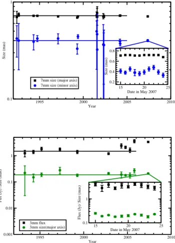
4.2.3 Source Size Measurements and Its Possible Variability . . . . 53

4.2.4 Variations of the Source Size . . . . 56

4.2.4.1 Time Dependence . . . . 56

4.2.4.2 Frequency Dependence . . . . 59

4.2.5 Intrinsic Source Size . . . . 62

4.2.6 Closure Quantities . . . . 63

4.2.6.1 Closure Phase . . . . 63

4.2.6.2 Closure Amplitude . . . . 67

4.2.7 Variability of VLBI Source Flux and NIR Variability . . . . . 69

4.3 Conclusion . . . . 71

5 The NRAO 530 72

5.1 Introduction . . . . 72

5.2 Observations and Data Analysis . . . . 74

5.3 Results and Discussion . . . . 76

5.3.1 Component Spectra and Spectral Reversal . . . . 77

5.3.2 Frequency-dependence of Component Positions . . . . 79

5.3.3 Flux Density and Structure Variability on Daily Timescales . . 83

5.3.4 Morphology and Its Evolution . . . . 85

5.3.5 Jet Kinematics at 15 GHz . . . . 90

5.4 Conclusion . . . . 94

6 Summary and Future Outlook 97 6.1 Summary . . . . 97

6.2 Future Outlook . . . . 98

Bibliography 101

7 Appendix-A 113

8 Appendix-B 115

9 Appendix-C 124

10 Erkl¨arung 141

11 Curriculum Vitae 142

List of Tables

2.1 Apparent angular sizes of event horizons for some black hole candidates 11 4.1 Flux density ratios between LL and RR for NRAO 530 and Sgr A* . . 45 4.2 Average source model parameters of Sgr A*. . . . . 49 4.3 Flux density variability characteristics of Sgr A*. . . . . 49 4.4 Structure variability characteristics of Sgr A*. . . . . 55 4.5 Averaged closure phases for some representative triangles at 86 GHz . 66 5.1 Position shift of jet components . . . . 82 5.2 Flux variability characteristics of model fit components of NRAO 530. 85 5.3 Variability characteristics of core separation for the jet components . . 86 5.4 P.A. variability characteristics of model fit components for NRAO 530 86 5.5 Linear fit results on the core separation of the jet components . . . . . 91 6.1 Properties of existing and proposed radio telescopes suitable for VLBI

at ν ≥ 230 GHz . . . 100

8.1 Description of VLBA images of Sgr A* . . . 121

8.2 Results from the modeling of the VLBA observations of Sgr A*. . . . 122

9.1 Description of VLBA images of NRAO 530 . . . 130

9.2 Model-fitting results for NRAO 530 . . . 132

List of Figures

1.1 A schematic view of the unification scheme . . . . 5

2.1 Black hole mass determination at the Galactic center. . . . . 13

2.2 The apparent motion of Sgr A* relative to J1745-283 . . . . 14

2.3 Angular broadening in Sgr A* . . . . 17

2.4 Spectrum of Sgr A* . . . . 21

3.1 A plot of resolution vs. frequency for astronomical instruments . . . . 31

4.1 uv coverage plots at 86 GHz . . . . 44

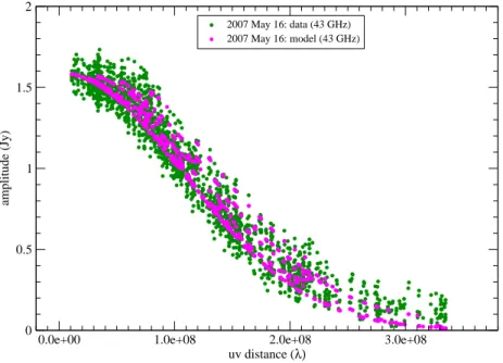
4.2 A plot of correlated flux density vs. uv distance at 43 GHz . . . . 47

4.3 Light curves for Sgr A* and NRAO 530 at 22, 43, and 86 GHz . . . . 48

4.4 Spectrum of Sgr *A . . . . 51

4.5 Spectral index α as a function of flux density at 86 GHz . . . . 52

4.6 Measured apparent structure of Sgr A* at 22, 43, and 86 GHz . . . . . 54

4.7 Measured angular size plotted vs. flux density at 22, 43, and 86 GHz . 56 4.8 Position angle of the major axis of Sgr A* plotted vs. flux density . . 57

4.9 Variability of Sgr A* . . . . 58

4.10 Angular broadening in Sgr A* . . . . 59

4.11 Ratio between the apparent size of Sgr A* and scattering size . . . . . 61

4.12 Ratio between the apparent size of Sgr A* and the new scattering size 61 4.13 Intrinsic size of Sgr A* plotted vs. wavelength . . . . 63

4.14 Closure phases at 86 GHz . . . . 64

4.15 Closure amplitudes at 43 GHz . . . . 68

4.16 Closure amplitudes for the FD, KP, LA, and PT quadrangle at 86 GHz 68 4.17 NIR light curve of the May 15, 2007 flare . . . . 69

4.18 Combined light curve of Sgr A* from the May 2007 campaign . . . . 70

5.1 Morphology of NRAO 530 from pc to kpc scales . . . . 73

5.2 Light curve of NRAO 530 at 5, 8, and 15 GHz . . . . 75

5.3 Components’ Spectra . . . . 78

5.4 Plot of spectral index vs. core separation . . . . 79

5.5 Frequency dependence of jet components . . . . 81

5.6 Slice for the inner jet of NRAO 530 along P.A. = − 10

. . . . 84

5.7 Flux density of model fit components plotted vs. time . . . . 87

5.8 Core separation and position angle of jet components plotted vs. time 88 5.9 Comparison of projected trajectory of jet components . . . . 89

5.10 Evolution of the projected jet axis . . . . 90

5.11 Core separation vs. time for jet components in NRAO 530 . . . . 92

5.12 Relativistic effects in NRAO 530 . . . . 93

5.13 Position angle vs. time for jet components in NRAO 530 . . . . 94

5.14 Time evolution of 15 GHz flux density of model fit components . . . . 95

5.15 Total VLBI flux density and position angle of the component d vs. time 95 8.1 Clean images of Sgr A* . . . 115

8.1 -continued . . . 116

8.0 -continued . . . 117

8.0 -continued . . . 118

8.0 -continued . . . 119

8.0 -continued . . . 120

9.1 Clean images of NRAO 530. . . . 124

9.1 -continued . . . 125

9.1 -continued . . . 126

9.1 -continued . . . 127

9.2 Clean images of NRAO 530 at 15 GHz. . . . 128

9.2 -continued . . . 129

1 Introduction

AGNs exist in the centers of at least 10 per cent of all galaxies

, in many cases out- shining their entire host galaxy. Systematic studies of bright nuclei of galaxies can be traced back to as early as 1940s when Seyfert (1943) studied non-stellar activity in a sample of galactic nuclei. However, the recognition of the significance of Seyfert’s work had to wait until Baade & Minkowski (1954) identified “active galaxies” as the optical counterparts of several bright radio sources. Soon after, Baade (1956) identified the polarized optical and radio emission from the jet of M 87, verifying the synchrotron emission mechanism. This allowed Burbidge (1956) to point out that extragalactic ra- dio sources contain tremendous amounts of energy (up to ∼ 10

erg). Such huge energy requirements led to the “energy crisis”, widely discussed in the early 1960s, especially with the discovery of quasi stellar objects (QSOs) (Schmidt 1963).

The concept that massive, (stellar-type) objects (up to ∼ 10

M

) power quasars or AGN, through gravitational energy was for the first time introduced by Hoyle & Fowler (1963). Zel’Dovich & Novikov (1965), Salpeter (1964), and Lynden-Bell (1969) fur- ther proposed that the huge energy release from an AGN could be explained by the accretion of matter onto a supermassive black hole (SMBH). In this picture the radio emission from AGNs is produced by a relativistic jet due to synchrotron emission of relativistic electrons moving in a magnetic field within the jet (Blandford & K¨onigl 1979). Similarly to these luminous AGNs, Lynden-Bell & Rees (1971) considered the black hole model to be applicable also for the nucleus of the Milky Way. A compact synchrotron radio source powered by gas spiraling into a black hole was proposed as one of the “critical observations” which could test the validity of the black hole scenario. Three years later, Balick & Brown (1974) did detect such a compact radio source in the direction of the Galactic Center (GC, Morris & Serabyn 1996; Melia &

Falcke 2001).

1http://ircamera.as.arizona.edu/NatSci102/lectures/agns.htm

1.1 Active Galactic Nuclei

As we will see in this section, although all AGNs consist of the same ingredients, different subclasses have distinct observational properties. Like all other fields of sci- ence, one of the primary goals of AGN studies is to develop a theory that could explain the diversity in observed properties through a single and simple model. In the current unified scheme of AGNs (Antonucci 1993; Urry & Padovani 1995), the different ob- servational properties are interpreted as the result of different viewing angles, i.e., as a geometrical effect. In the following, the basic observational properties for a variety of subclasses are outlined and explain in the context of the unified scheme.

1.1.1 Observational Properties

Seyfert galaxies are mostly spiral galaxies. They are named after Seyfert (1943), who first pointed out that several similar galaxies with bright central regions possibly form a distinct class. The presence of broad emission lines (width from several hundreds to up to 10

km/s) from the bright nucleus is the key to classify a galaxy as a Seyfert. Seyfert galaxies are further divided into two subclasses (type 1 and type 2) by Khachikian &

Weedman (1974), depending on whether the spectra show both “narrow” (several hun- dreds km/s) and “broad” emission lines (type 1), or only “narrow” lines (type 2). It is now believed that both types are in essence the same and their apparent difference is caused by different viewing angles. As we will see in the unified scheme, type 1s are those observed from a face-on view of the obscuring torus, while those observed from an edge-on view are classified as type 2s. Therefore, the presence of an opti- cally thick dust torus surrounding the AGN core, that obscures the broad line region (BLR), is critical for the unification of Seyfert galaxies. The presence of the torus is strongly supported by the detection of polarized broad emission lines in the spectrum of NGC 1068, whose spectrum resembles a type 2 Seyfert (Antonucci & Miller 1985).

The polarized flux comes from dusty clouds which scatter and polarize the light from the nucleus. In the unified scheme, Seyferts are dim, radio-quiet quasars.

Radio galaxies do not share many common characteristics, apart from being highly luminous in radio wavelengths. Their hosts are elliptical galaxies and their radio struc- ture often shows double-sided radio lobes on kpc scales, with one or (rarely) two jets tracing back to the optical nucleus. The single-sidedness of the radio jet on pc scales is normally interpreted as a consequence of relativistic de-boosting effects. Fanaroff

& Riley (1974) divided the radio galaxies into two subclasses (FR-I and FR-II) based

on the morphology of their lobes. FR-Is are weaker radio sources with the so-called

“edge-darkened” extended emission and two-sided jets. On the other hand, FR-IIs are more luminous, showing edge-brightened extended emission. Most of them show symmetric lobes with co-linear structure (parallel jet axis) with hot spots either at the edge of the radio lobes or embedded within their radio structure.

Based on the width of their optical emission lines, radio galaxies can form two further sub-categories, Broad Line Radio Galaxies and Narrow Line Radio Galaxies.

The former display emission lines with widths similar to those in Seyfert 1 galaxies and the latter show emission line widths similar to those in Seyfert 2 galaxies. These are thought to be radio loud counterparts of Seyfert galaxies.

Quasars were first discovered as strong radio sources, though most quasars ( ∼ 99 %) are now known to be radio quiet when compared to their optical luminosity.

Historically, the radio quiet quasars were called Quasi-Stellar Objects (QSOs), in con- trast to Quasi-Stellar Radio Sources (Quasars). Now we know that they are the same kind of objects. These sources are some of the most powerful and distant AGNs. The fact that quasars are visible at enormous cosmological distances, as suggested by their high redshifts, implies a huge luminosity. In addition, the short timescales of vari- ability (as short as hours) of their flux indicates that their enormous energy output originates in a very compact region.

Quasars are strong emitters at all wavelengths and show strong and broad emission lines of highly ionized elements (Ca, Mg, O), which is the most important observa- tional characteristic to distinguish quasars from stars and normal galaxies. Both broad and narrow emission lines are present in their optical spectrum, similar to a Type 1 Seyfert galaxy. In this sense, quasars are powerful versions of Seyfert galaxies. The radio morphology of quasars is similar to FR-II sources with the exception that the luminosity ratio between core and jet, and lobes is higher in quasars.

Blazars is a generic term for BL Lac objects (BL Lacs) and Optically Violently Variable quasars (OVVs). Their host galaxies are often giant elliptical galaxies. BL Lac objects (named after the prototype, BL Lac) are highly variable and highly polar- ized. They show relatively flat and featureless spectra when compared to other AGNs.

They are also compact radio sources with non-thermal continuous spectrum ranging

from the radio to the γ-rays. These properties are attributed to emission from a rel-

ativistic jet oriented close to the line of sight. OVV quasars are similar to BL Lac

objects in the sense that they show large and rapid optical variability. However, their

spectra have features (e.g., strong broad emission lines), which are different from those

in BL Lacs. It is generally believed that OVV quasars are intrinsically powerful radio

galaxies while BL Lac objects are intrinsically weak radio galaxies.

1.1.2 A Unified View

The basic composition of an AGN (as illustrated in Figure 1.1) includes a SMBH (10

– 10

M

) in the very center, which powers the AGN by accreting surrounding matter via a circumnuclear accretion disk. The viscous friction in the accretion disk is thought to be the mechanism, which turns gravitational energy into radiation. Accretion can convert up to 30 % of the rest mass of the in-falling gas into radiation (Thorne 1974), much larger than the efficiency of nuclear fusion (< 1 %). For a quasar with typical mass of M

= 10

M

, the Eddington luminosity L

, at which the radiation pressure force balances the gravitational force, is

T

∼ 1.3 × 10

⊙

∼ 1.3 × 10

erg s

, where M

the black hole mass, m

the proton rest mass, and σ

the Thomson cross section. Some material is accelerated by strong magnetic fields and ejected perpendic- ular to the accretion disc in the form of highly collimated jet. The jet can reach large distances, in some extreme cases, up to mega-parsec scales. Further outwards from the central engine is the BLR, surrounded by an opaque molecular torus. Above the torus is a layer of low-velocity gas which is refereed as “narrow line region” (NLR).

The opaque molecular torus and the relativistic jets seem to be two key ingredients for the classification and unification of AGNs. For a range of viewing angles, the opaque torus blocks the view towards the BLR, and we can only see the low velocity gas from the NLR. When observed at a line of sight close to the jet direction, AGNs show broad spectral lines in the optical spectrum (Type 1 AGN, e.g., Seyfert 1s, Broad Line Radio Galaxies and Type 1 Quasars), whereas when observed edge-on, the system only shows narrow emission lines from the low velocity gas in the NLR (Type 2 AGN, e.g., Seyfert 2s, Narrow Line Radio Galaxies and Type 2 Quasars). Sometimes one speaks also about Type 0 objects, which is a special case, in which we are looking directly into the jet.

AGNs can also be divided according to the radio power: “radio-loud” or “radio quiet” in terms of their ratio of radio to optical luminosity. The existence of doppler enhanced relativistic jets seems to be responsible for the radio loudness (Kellermann et al. 1989) and the radio dichotomy is perhaps related to jet production efficiency.

However, it is not well understood what is the key parameter that determines the jets production. The black hole mass (Laor 2000; Liu et al. 2006b) and spin (Blandford

& Znajek 1977) could be of relevance. Investigations of the jet activity in X-ray bina- ries suggest that the accretion rate controls the jet production efficiency (Fender et al.

2004). For radio loud AGNs, relativistic beaming effects play an important role in the

radio appearance. It is accepted that low power FRIs and BL Lacs form a subgroup

of objects where the relativistic jet is viewed at small angles to the observer’s line of

sight. At larger viewing angles, the radio emission is dominated by the large-scale lobes and therefore, it is a classical FRI radio galaxy. Correspondingly, OVVs, radio- loud quasars, FRIIs appear to form another powerful subgroup with increasing view angle.

Jet

Obscuring Torus

Black Hole

Narrow Line Region

Broad Line Region

Accretion Disk

Figure 1.1: A schematic view of the unification scheme (Urry & Padovani 1995).

1.2 Basics of Relativistic Jets

1.2.1 Synchrotron Emission

Synchrotron emission (the relativistic equivalent of cyclotron emission) is generated by charged particles spiraling in a magnetic field at nearly the speed of light. It has become the research tool for the study of extragalactic jet physics since its first ob- servation from a General Electric synchrotron accelerator in 1940s. Synchrotron ra- diation is observed in astronomical sources, such as jets of compact radio sources, supernova and supernova remnants, stars (non-thermal emission), galaxies and cluster halos. Synchrotron radiation shows characteristic polarization in the plane perpendic- ular to its propagation, which was used often in order to confirm its presence (e.g., Baade 1956).

Here we outline some characteristics of the synchrotron mechanism. Detailed

derivation of the formulae can be found in (e.g., Pacholczyk 1970; Rybicki & Light-

man 1979). Due to the relativistic motion of the emitting particles, the radiation is

strongly beamed into a cone in the forward direction (abberation) with angular width

of about

radians, where γ is the Lorentz factor of the electrons. The emission from a

single electron

has a characteristic frequency:

ν

= γ

eB

2πm

c , (1.1)

where e is the electron charge, m

is the electron mass, γ ≡ √

1−β²_e

the Lorentz factor of the electron with velocity β

, in units of speed of light c, and B the magnetic field. A power-law distribution of particle energies over a large range (N(E)dE ∝ E

dE, where N(E)dE is the number of electrons per unit volume with energies E to E+dE) will pro- duce a superposition of individual electron spectra and produce emission described by a power-law. The optically thin spectral index α (S

∝ ν

) is

. At low frequencies the synchrotron emission is self-absorbed and below the turnover frequency ν

, it has a spectral index of 2.5 for a spatially homogeneous source, regardless of the energy distribution of the electrons. In the case of an isotropic distribution of pitch angles (the angle between the magnetic field and the velocity), the average power emitted by an electron follows:

P

= 4

3 σ

cγ

β

U

, (1.2)

where σ

is the Thompson cross section and U

=

is the energy density of the mag- netic field. Thus, one can estimate the time scale of cooling via synchrotron radiation:

t

= E

h P

i = γm

c

4

3

σ

cU

γ

β

∼ 24.6

B

γ yr. (1.3)

From this it directly follows that cooling is faster at higher energies, and consequently, the spectrum gets steeper with increasing time. The relativistic electrons also lose energy through Inverse Compton scattering, a process that occurs when a low-energy (radio) photon (hν ≪ m

c

) is scattered by a relativistic electron. The scattering tends to upshift the photon frequency roughly by γ

. One can derive the total power emitted through this process:

P

= 4

3 σ

cγ

β

U

, (1.4) where U

is the radiation energy density. It is immediately obvious that:

P

P

= U

U

. (1.5)

Thus, one can judge which process dominates energy loss through the ratio of the energy density of the magnetic field to that of the radiation field.

2Electrons can be accelerated to relativistic speeds easier than protons of the larger mass of the latter and thus synchrotron emission is much stronger for electrons than for equal energy protons.

Synchrotron radiation is also characterized by its high linear polarization. At the optically thin part of the spectrum, the polarization percentage (m) in a uniform mag- netic field is given by:

m(%) = 100 × s + 1

s +

. (1.6)

For a typical value of s = 2, one finds that the fractional polarization for optically thin emission can be as high as 69 %.

1.2.2 Relativistic E ff ects

For a bright knot moving with a speed v . c, it is possible that transverse speeds (to the line of sight) speeds appear to be faster-than-light. The apparent superluminal motion, as predicted by Rees (1966), is an illusion resulting from a simple geometric effect.

The discovery of superluminal motion was made in early 1970s by repeated VLBI observations of the quasars 3C 279 and 3C 273 (Whitney et al. 1971; Cohen et al.

1971). The observed transverse velocity of an emitting feature is:

β

= β sin θ

1 − β cos θ , (1.7)

where β

and β are the apparent and the true velocity in units of speed of light c and θ is the angle between the direction of motion and the line of sight.

When a source is approaching us at a speed of v ( . c) with an angle θ to the line of sight, the observed frequency ν of a periodic signal is related to the frequency ν

in the co-moving (primed) frame by ν = δν

, where δ is the relativistic Doppler factor:

δ = 1

Γ(1 − β cos θ) , (1.8)

with Γ ≡ √

1−β²

the bulk Lorentz factor. One can show that the quantity

is a Lorentz invariant (Rybicki & Lightman 1979, chap. 4.9). Therefore, the observed flux density (S ) is enhanced (relativistic beaming) as:

S = S

δ

, (1.9)

where S

is the flux density in the co-moving frame, and p = 3 − α. The spectral index α appears on the equation because the boosting increases the observed frequency. For a continuous jet, p changes to 2 − α (Lind & Blandford 1985). Equation 1.9 allows us to derive a flux density ratio (R) between the jet and counter jet for an assumed intrinsically symmetric jet, as:

R = ( 1 + β cos θ

1 − β cos θ )

. (1.10)

Obviously, the jet is significantly brighter than the counter jet even for a mildly rela- tivistic jet. This explains why we almost always see one-sided jets.

1.2.3 Brightness Temperature

The radiation from a black body in thermodynamic equilibrium is given by Planck’s law:

I

= 2hν

c

1

exp

− 1 , (1.11)

where I

is the brightness in W.m

.Hz

.sr

, h is the Planck constant (6.63 × 10

J sec), ν is the frequency in Hz,

c is the speed of light in vacuum (2.998 × 10

m sec

), k is the Boltzmann constant (1.38 × 10

J K

), T is the temperature in Kelvin.

In the radio regime, where hν ≪ kT , Plank’s law reduces to the Rayleigh-Jeans ap- proximation:

I

= 2ν

kT

c

(1.12)

The brightness of a black body depends only on its temperature and the observing frequency. Hence, for an observed brightness one can define an equivalent temperature that a black body is needed to have in order to emit the observed intensity at a given frequency:

T

= I

c

2ν

k . (1.13)

The brightness temperature of a VLBI source component with Gaussian brightness distribution is given by:

T

= 1.22 × 10

S

ν

θ

K, (1.14)

where S is the flux density in Jy, ν the frequency in GHz, and θ (FWHM) in mas, respectively.

The brightness temperature is a good diagnostic for the emission process at work in compact radio sources. VLBI measurements of flux densities and angular sizes for extragalactic radio sources have consistently yielded peak brightness temperatures in the range of 10

K, which is definitively produced by non-thermal processes since kT > m

c

.

Theoretically, there are strong upper limits on the brightness temperature for an

incoherent synchrotron source. They are the inverse Compton limit, which was first

pointed out by Kellermann & Pauliny-Toth (1969), and a tighter limit based on equipar- tition arguments (Readhead 1994). The inverse Compton limit is based on the argu- ment that at brightness temperatures T

> 10

K, the energy loss of electrons will be dominated by inverse Compton scattering effects (Equation 1.5). This process will cool the system rapidly and therefore bring the brightness temperature below this limit.

Readhead (1994) derived an even tighter limit on the maximum brightness tempera- ture. According to him, sources radiate below 5 × 10

–10

K when energy densities of the relativistic particles and the magnetic fields are in equipartition. Measured bright- ness temperature in excess of these limits can be explained by Doppler boosting.

There are also observational limitations to the maximum brightness temperature that can be measured interferometrically. According to Equation 1.14, one finds that the measured brightness temperature depends only on the maximum baseline length (D), for a given flux density, since the resolution is proportional to

. Therefore, the maximum brightness temperature that can be probed from earth based interferometer is limited by the diameter of the Earth and is coincidentally ∼ 10

K (Kellermann &

Moran 2001). In other words, ground-based baselines can not resolve a source with

brightness temperature ≫ 10

K.

2 Sagittarius A* as an AGN

Located at the dynamical center of the Galaxy, the compact radio, NIR, and X-ray source Sagittarius A* (hereafter Sgr A*

) is believed to be the emission counterpart of a ∼ 4 × 10

M

black hole (see section 2.2.1). As mentioned in Chapter 1, the discovery of Balick & Brown (1974) provided strong support for the black hole scenario and it was a detection using the “right” interferometer after several attempts (see e.g., Goss et al. 2003, for a detailed recounting). Its relative proximity renders it able to be investigated in great detail.

In terms of Eddington luminosity, Sgr A* is extremely dim. Its bolometric lumi- nosity L is ∼ 10

erg s

, which is 8 orders of magnitude lower than its Eddington luminosity (L

∼ 5.2 × 10

erg s

). The ultra-low luminosity of Sgr A* had raised some doubts about the accretion - black hole paradigm acting at the GC. However, in spite of this apparent diversity, there is now strong evidence that Sgr A* is associated with a SMBH (see next section). Therefore, Sgr A* and AGNs do share a common en- ergy production mechanism, i.e., the accretion of matter onto a SMBH at their centers.

Moreover, Sgr A* fits well into the so-called “fundamental plane” (a relationship be- tween radio and X-ray luminosities and mass), indicating a similar physical process at work in accreting black holes of all masses (Fender et al. 2007, and references therein).

In this context, Sgr A* serves as a link between stellar mass and 10

M

black holes.

2.1 The Uniqueness of Sgr A*

Sgr A* stands out from its surrounding radio sources and is unique in several ways.

Its compactness (point-like) and non-thermal spectrum are reminiscent of the com- pact nuclear radio sources associated with typical AGNs. The proximity of Sgr A* (8 kpc), however, offers us a unique opportunity for testing the SMBH paradigm, which is unaccessible in the case of AGNs. For example, the next closest galactic nucleus

3A few names (e.g., “GCCRS” (Reynolds & McKee 1980), “Sgr-A” (Brown et al. 1978), “Sgr A”

Brown & Lo(1982), “Sgr A (cn)” (Backer & Sramek 1982)) were assigned to the compact radio source but only “Sgr A*” (Brown 1982) survived.

(M 31*) is ∼ 100 times farther away from us than Sgr A*. As shown in Table 2.1, apparent angular sizes of several black hole event horizons are compared for several (notable) sources. In terms of apparent size, Sgr A* is the largest black hole candidate.

Within the next decade, imaging of the event horizon of Sgr A* would even be pos- sible (Doeleman et al. 2009a). Thus, the study of physics near the event horizon will finally provide important insight into other black hole accreting systems.

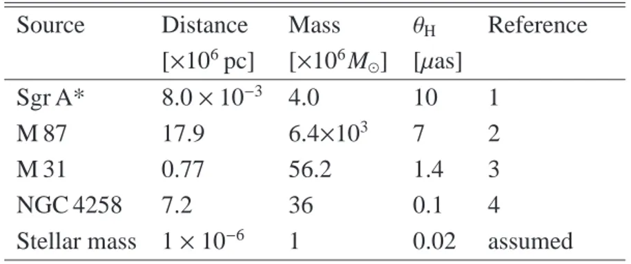
Table 2.1: Apparent angular size of the event horizon of some black hole candidates

Source Distance Mass θ

Reference

[ × 10

pc] [ × 10

M

] [µas]

Sgr A* 8.0 × 10

4.0 10 1

M 87 17.9 6.4 × 10

7 2

M 31 0.77 56.2 1.4 3

NGC 4258 7.2 36 0.1 4

Stellar mass 1 × 10

1 0.02 assumed

References: (1) section2.2.1; (2) Both mass and distance fromGebhardt & Thomas(2009); Note the suddenly double of the mass. (3)Salow & Statler(2004, and references therein); (4) mass fromMiyoshi et al.(1995) and distance fromHerrnstein et al.

(1999). Adapted and updated fromMiyoshi & Kameno(2002).

Recently, there has been accumulation of evidence that Sgr A* is the emission counterpart of a ∼ 4 × 10

M

black hole at the GC. Specifically, the evidences come mainly from the study of stellar dynamics in the vicinity of Sgr A* and proper mo- tion of Sgr A* (section 2.2.1). Recent improvement on the size determination of Sgr A* with VLBI allows us to set stringent constrains on the mass density with the help of proper motion studies (Bower et al. 2004; Shen et al. 2005; Doeleman et al.

2008). The implied mass density of 9.3 × 10

M

pc

(Doeleman et al. 2008) is just 2 orders of magnitude lower than that of a 4 × 10

M

black hole within its Schwarzschild radius.

The uniqueness of Sgr A* also lies in the typical timescales of order of minutes to hours for the orbital motion near the last stable orbit of the 4 × 10

M

black hole.

For instance, rapid variability is expected to occur at the last stable orbit with a period

of ∼ 30 minutes (for a non-rotating black hole). In the case of a maximally rotating

Kerr black hole, the time scales are within ∼ 4 (prograde) to 54 (retrograde) minutes

depending on its spin (Melia et al. 2001, scaled with 4 × 10

M

). Compared to the

time scale associated with stellar mass black holes and luminous AGNs, these are

easily accessible to us. Therefore, Sgr A* is an ideal “poster child” for black hole

studies with unique advantages both spatially and temporally.

2.2 Observational Facts about Sgr A*

2.2.1 Mass

The most robust evidence for the existence of a SMBH at the GC comes from the highly concentrated gravitational mass determined through investigations of gas and stellar dynamics in the near infrared (NIR). Evidence has been accumulated over the past three decades from observations of radial velocities of gas and stars (Genzel &

Townes 1987). However, reliable determination of the mass content and concentration relies on the measurement of the full velocity field with test particles (stars, since gas is subject to other non-gravitational forces). Here we list some milestones towards this goal.

• Proper motion studies (Eckart & Genzel 1996; Ghez et al. 1998)

Before proper motion measurements were available, there were only radial ve- locity measurements of gas and stars. The proper motion measurements re- laxed the assumption that stellar obits are largely circularly and isotropically distributed (see Figure 2.1 (b)). The dependence of velocity dispersion on the distance from Sgr A* is in good agreement with that obtained from radial veloc- ities, and therefore solidifies the evidence for the existence of a massive point mass.

• Accelerations (Ghez et al. 2000; Eckart et al. 2002)

Acceleration measurements of stars permit the determination of the location of the dark mass.

• Keplerian orbits (Sch¨odel et al. 2002; Ghez et al. 2005)

Keplearian orbits or even full orbital solutions allow then to constrain the posi- tion and mass of the black hole.

The mass density distribution (Figure 2.1 (a)), as inferred from velocity dispersion measurements, excludes explanations other than that of a SMBH. As of 2009, as many as 26 stellar obits in the GC have been obtained (Eckart & Genzel 1996, 1997; Eckart et al. 2002; Sch¨odel et al. 2002; Eisenhauer et al. 2003; Ghez et al. 2000, 2005, 2008;

Gillessen et al. 2009). All the orbits can be well fitted by a single point mass and focal

position (as illustrated in Figure 2.1 (b)). Registration of the radio reference frame and

NIR frame (Reid et al. 2007, and references therein) allows comparison of the position

of the central point mass inferred from orbit fits to the radio source Sgr A*. They are

found to coincide within roughly 20 AU (2 mas). Measurement of the radial velocity

of the young stars (Ghez et al. 2003b) also allows the geometric determination of the distance to the Galactic Center (R

) from stellar orbits (Eisenhauer et al. 2003, 2005).

(a)

S2

S1 S4

S8

S9

S12

S13

S14 S17

S21

S24 S31

S33 S27

S29 S5

S6

S19

S18 S38

0.4 0.2 0. -0.2 -0.4

-0.4 -0.2 0.

0.2 0.4

R.A.H"L

DecH"L

(b)

Figure 2.1: (a) The enclosed masses from individual stars orbital motion (filled sym- bols) and those determined based on velocity dispersion (open symbols) in the nuclear cluster in the Galactic Center. The solid line represents the best fit black hole plus luminous cluster model, with black hole mass M

= (3.6 ± 0.4) × 10

M

. The dashed line indicates the enclosed mass due to a star cluster alone (from Ghez et al. 2003a).

(b): A plot of the stellar orbits of the stars in the central arcsecond of the GC. The co- ordinate system was chosen so that Sgr A* is at rest. The arrows indicate the direction of motion. Taken from Gillessen et al. (2009).

Complementary to stellar dynamics studies, proper motion studies of Sgr A* via VLBI phase referencing can provide an independent constrain on the mass of Sgr A* it- self. If the compact radio source Sgr A* is indeed the gravitational source, it should be nearly at rest at the dynamical center of the Galaxy, and any peculiar motion can provide a mass estimate (Backer & Sramek 1982). The apparent proper motion of Sgr A* observed with the VLA (Backer & Sramek 1999) and VLBA (Reid et al. 1999;

Reid & Brunthaler 2004) was shown to be consistent with that expected from the known effects of the Sun’s motion relative to Sgr A*, namely the peculiar motion rela- tive to the local standard of rest and secular parallax of Sgr A* due to the rotation of the Sun around the GC. After removing these effects, Reid & Brunthaler (2004) found that the residual proper motion of Sgr A* perpendicular to the Galactic plane is as small as

− 0.4 ± 0.9 km s

(Figure 2.2), which leads to the conclusion that Sgr A* contains at

least a mass of ∼ 4 × 10

M

.

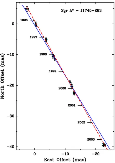
Figure 2.2: Sgr A* position residuals on the sky plane with respect to the background

source, J1745-283. Shown as a dashed line is a weighted least squares fit proper motion

and the solid line gives the orientation of the Galactic plane. The clear deviation of

the motion from the Galactic plane can be well explained by the known component

of the solar motion perpendicular to the Galactic plane. After removing the known

Z-component of the solar motion, the out-of-plane component of the peculiar motion

of Sgr A* is as small as − 0.4 ± 0.9 km s

(from Reid & Brunthaler 2004).

Recent revision of the central black hole’s mass and distance has yielded consistent values: M

= (4.31 ± 0.06 |

± 0.36 |

) × 10

M

and R

= 8.33 ± 0.35 kpc (Gillessen et al. 2009), M

= (4.5 ± 0.4) × 10

M

and R

= 8.4 ± 0.4 kpc (Ghez et al. 2008), and R

= 8.4 ± 0.6 kpc (Reid et al. 2009). Throughout this thesis we adopt for the GC black hole a total mass of 4 × 10

M

and a distance of 8 kpc to us. The Schwarzschild radius (R

=

c²

) is then 1.2 × 10

m, or 0.1 AU, or 10 µas, and 1 light-minute is 1.5 R

. 2.2.2 Scattering E ff ects

Radio waves from Sgr A* are heavily scattered by the intervening ISM. Interstellar scattering arises from fluctuations of the electron density. It causes many observable effects such as the angular broadening of a source, temporal broadening of a pulse sig- nal, flux density fluctuations (scintillation, both diffractive and refractive), and image wander (Rickett 1990). Electron density fluctuations are normally thought to occur over a wide range of scales. Its three dimensional spatial power spectrum P

often takes the form of a power-law with cutoffs (e.g., Armstrong et al. 1995):

P

(q) ≈ C

q

, L

< q < ℓ

(2.1) where q is the spatial wavenumber and the constant C

is a measure of the electron density fluctuations. L

is the “outer” scale on which the fluctuations occur, and ℓ the

“inner” scale on which the fluctuations dissipate. If β < 4, the spectrum is referred to as shallow and diffractive scattering effects would dominate. If β > 4, it’s a steep spectrum with refractive effects dominant. β =

corresponds to a Kolmogorov spectrum (Desai

& Fey 2001, and references therein). Along many lines of sight, the spectrum index of the power spectrum were found to be close to the Kolmogorov value (Wilkinson et al.

1994; Molnar et al. 1995; J. Franco & A. Carraminana 1999; Lazio & Fey 2001). For a few lines of sight the spectral index is found to be approaching or large than 4 (Moran et al. 1990; Clegg et al. 1993; Desai & Fey 2001).

2.2.2.1 Angular Broadening

Angular broadening, as its name implies, leads to an enlarged angular size of a source.

At a given wavelength, the intrinsic size θ

can be obtained via the deconvolution operation:

θ

= q

θ

− θ

(2.2)

where θ

and θ

are the measured apparent size and the scattering disk size, respec-

tively (e.g., Narayan & Hubbard 1988). The wavelength dependence of the scattering

size for a shallow wavenumber spectrum, is: θ

∝ λ

. When the VLBI baseline length becomes comparable to the inner scale of the density fluctuations, the scatter- ing law changes and has the following form: θ

∝ λ

(Lazio 2004).

Soon after the discovery of Sgr A*, it was realized that the observed change of size with wavelength is due to interstellar scattering effects (Davies et al. 1976). Further- more, Lo et al. (1985, 1993) found that the scatter-broadened image of Sgr A* can be modeled by an elliptical Gaussian with an axes ratio of ∼ 0.5 at 8 GHz, indicating an anisotropic scattering effect. The existence of anisotropic scattering towards the GC region was further established when non-circular scattering disks of OH masers within 25

of Sgr A* were observed. It is, therefore, evident that the electron density inhomo- geneities have a preferred direction. Such anisotropy in electron density fluctuations could result, e.g., from an ordered magnetic field (Frail et al. 1994; van Langevelde et al. 1992).

Radio images of several other sources also display the effects of anisotropic scat- tering. The brightness distribution is close to an elliptical Gaussian with axes ratio varying from source to source, e.g., 2013+370 (Spangler & Cordes 1988), Cygnus X-3 (Wilkinson et al. 1994; Molnar et al. 1995), NGC 6334B (Trotter et al. 1998).

Moreover, axes ratio and orientation of the scattering disk have been found to exhibit λ-dependence toward a few more lines-of-sight, e.g., Cygnus X-3 (Wilkinson et al.

1994) and NGC 6334B (Trotter et al. 1998). This has been attributed to an increas- ingly ordered magnetic field on smaller scales (cf. Figure 13 in Trotter et al. 1998).

Such scale-dependent anisotropy interpretation could in principle enable one to esti- mate the outer scale of the density fluctuations. An alternative interpretation for the change of orientation and ellipticity with wavelength may be that the intrinsic structure begins to shine through at higher frequencies. For Sgr A*, no indication of wavelength dependence of the orientation was found in the past (for a possible deviation from this, see section 4.2.3 of Chapter 4).

The knowledge of the exact nature and location of the scattering material, however, is still poor. It has been argued that the scattering screen which causes angular broad- ening of Sgr A* occurs in the ionized surface of molecular clouds lying in the central 100 parsecs of the Galaxy (Yusef-Zadeh et al. 1994). The location of the scattering region close to GC was supported by later observations of Lazio & Cordes (1998), who constrained the scattering screen - GC distance to 150 parsecs.

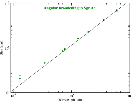
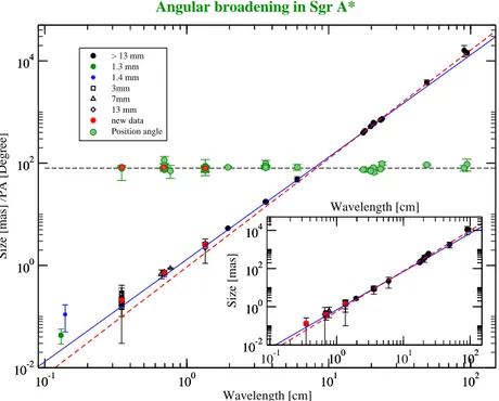
The apparent angular sizes along both the major and minor axis for the ellipti-

cal structure of Sgr A* show a wavelength dependence generally consistent with a λ

dependence at centimeter wavelengths. Deviations from a λ

scaling at shorter wave-

lengths (millimeter) are commonly interpreted as an effect of intrinsic structure becom-

10^-1 10⁰ 10¹ Wavelength (cm)

10^-2 10⁰ 10²

Size (mas)

10^-1 10⁰ 10¹

10^-2 10⁰ 10²

Angular broadening in Sgr A*

Figure 2.3: Apparent angular size of Sgr A*along the major axis as a function of wave- length. The data are from Bower et al. (2004); Shen et al. (2005); Doeleman et al.

(2008). The solid line delineates a λ

scatter law (Bower et al. 2006), which is derived from longer wavelengths (17.4–23.8 cm) measurements.

ing dominant (Marcaide et al. 1992; Krichbaum et al. 1993; Yusef-Zadeh et al. 1994;

Lo et al. 1998; Krichbaum et al. 1998b; Doeleman et al. 2001, and references therein).

Figure 2.3 shows the angular broadening effect in Sgr A*. As mentioned above, the intrinsic size of Sgr A* is obtained by subtraction of the scattering size from the scat- tering broadened size in quadrature (equation 2.2). Therefore, the scattering law along the line of sight toward the GC is crucial for determining the intrinsic structure (size and shape).

2.2.2.2 Refractive Interstellar Scintillation

Refractive interstellar scattering is associated with electron density fluctuations on sub-

parsec scales. These fluctuations act as lenses that focus or defocus the source image,

are produced on scales much larger than those responsible for diffractive effects, and

cause slow fluctuations of intensity (scintillation). The refractive scattering timescale

is determined by the time the sub-parsec scale density fluctuation takes to move across

our line of sight. Typically, the timescale is of the order of days for pulsars and from

months to years for extragalactic sources (e.g., Lazio & Fey 2001). In contrast, diffrac-

tive scintillation (in analogy to twinkling of stars) is more rapid on timescales of min- utes to hours. For a shallow spectrum (β < 4), refractive effects would in general be suppressed by diffractive effects caused by even smaller density fluctuations (Romani et al. 1986).

Long-term flux variations for Sgr A* seen at low frequencies (< 5 GHz) have been explained in terms of refractive interstellar scattering (Zhao et al. 1989). Nonetheless, the observed modulation index seems to be under-predicted by a thin screen model based on the Kolmogorov spectrum. Models in which the scattering medium extends out can account for the high modulation index and are recently investigated in the context of Sgr A* (Macquart & Bower 2006). Later monitoring data, more densely sampled, found, however, that the variations are more pronounced at higher frequen- cies, indicating that the intrinsic variations become important (Zhao et al. 1992; Falcke 1999). In addition, the inferred variability timescale does not follow an expected λ

dependence from scattering theory (Falcke 1999; Melia & Falcke 2001).

At 0.8 and 1.3 mm, Gwinn et al. (1991) failed to detect significant flux variations on time scales from 0.1 s to one day. They argued that refractive scintillation for Sgr A*

is quenched at these wavelengths as the source angular size presumably exceeds the scattering size. In this way, a lower limit to the source size ( ∼ 10 µas) can also be obtained.

Although variability at high frequencies is generally thought to be source intrin- sic as discussed below, the nature of radio (centimeter) variability of Sgr A* has been debated. Since radio waves from Sgr A* are heavily scattered, refractive scintillation should contribute to flux variations unless it is quenched. After the claim of quasi- periodic modulations, an intrinsic cause for the variations is favored (Falcke 1999;

Zhao et al. 2001). Therefore, both extrinsic and intrinsic variability should be respon-

sible for the modulations at centimeter wavelengths. The difficulty lies in determining

the contribution of scattering effects and separating them from the intrinsic variations

of the source. Macquart & Bower (2006) collated multi-wavelength (0.7–20 cm) mon-

itoring data available at that time. Their analysis indicates Sgr A* shows no quasi-

periodic oscillations on any timescale between 1 week and 200 days. Additionally,

extended-medium models account well for the broad characteristics of the variability

on timescales larger than a few days and a 10 % of the variability on timescales of a

few days at 0.7–3 cm seems to be source intrinsic.

2.2.2.3 Position Wander

In addition to long-term flux density variations, interstellar scattering causes refractive fluctuations of the apparent position of a radio source. The magnitude of this effect is sensitive to the power law index of β. In the case of a “steep” spectrum (β > 4), models predict strong refractive position shifts, which are far greater than the scattering disk θ

(Rickett 1990).

Scattering-induced position wander of Sgr A* seems to be much smaller than θ

and it should occur on timescales larger than 10

hours, if at all (Reid et al. 2008).

Proper motion studies of Sgr A* provide stringent limits on the long-term position wander. These observations indicate refractive effects to be negligible (Backer &

Sramek 1982, 1999; Reid et al. 1999). Small displacement of the image centroids at different frequencies provide further support for this argument (Backer & Sramek 1982, 1999). Moreover, Gwinn et al. (1988) studied refractive position wander for H

O masers in Sgr B2(N). Their VLBI observations set an upper limit of 18 µas for the maser spots wander, and thus ruled out “steep” density spectrum towards that line of sight.

The angular broadening effect, refractive scintillation (Macquart & Bower 2006) and lack of image wander of Sgr A* are consistent with a picture of a “shallow” density spectrum (β < 4) for the scattering medium towards the GC.

2.2.3 Intrinsic Structure

It is clear from the above discussion that attempts to measure the source structure at centimeter wavelength suffer from the angular broadening effect, which dominates the resulting images. The λ

dependence of the scattering effect has been driving VLBI observations of Sgr A* to shorter and shorter wavelengths, where the image blurring vanishes. The last few years have seen great progress in the size determination of Sgr A*. Millimeter-VLBI observations of Sgr A* at 43 and 86 GHz suggest a break in the λ

dependence of the scattering law. This implies that the intrinsic source structure becomes visible and begins to dominate over the scatter broadening effect above ν ≃ 43 GHz (Krichbaum et al. 1998c; Lo et al. 1998; Doeleman et al. 2001; Bower et al.

2004; Shen et al. 2005; Bower et al. 2006; Krichbaum et al. 2006). The recent detection

of Sgr A* with VLBI at 1.3 mm at a fringe spacing of ∼ 60 µas has pushed the limit of

the size of the compact VLBI emission down to ∼ 4 R

( ∼ 43 µas). This is smaller

than the theoretically expected size of the emission region around a 4 × 10

M

SMBH,

assuming it is not rotating (Doeleman et al. 2008). At present it is unclear whether the