Inversion Symmetry and
Antiferromagnetic Quantum Critical Points
Inaugural-Dissertation zur
Erlangung des Doktorgrades
der Mathematisch-Naturwissenschaftlichen Fakult¨ at der Universit¨ at zu K¨ oln
vorgelegt von
Inga Anita Fischer
aus G¨ ottingen
K¨ oln 2006
Prof. Dr. E. M¨ uller-Hartmann
Tag der m¨ undlichen Pr¨ ufung: 30. Juni 2006
0. Introduction 1
I. Metallic Magnets without Inversion Symmetry: MnSi 3
1. Introduction 5
1.1. Experimental observations . . . . 5
1.2. Theory . . . . 8
2. Electrons in the Ordered Phase 9 2.1. Band structure from coupling of the electrons to the helix . . . . 9
2.2. Form of the spin-orbit coupling term in the bandstructure . . . . 12
2.3. Electron band structure and the Fermi surface . . . . 12
2.3.1. Band structure . . . . 15
2.3.2. Shape of the Fermi surface . . . . 16
2.4. Fermi surface: Experimental consequences . . . . 17
2.4.1. De-Haas–van-Alphen Effect . . . . 18
2.4.2. Impurity scattering . . . . 21
2.4.3. Conductivity . . . . 21
2.4.4. Anomalous Skin effect . . . . 22
2.5. Minibands and Damping . . . . 23
2.6. Discussion . . . . 26
3. New Phases from a Ginzburg-Landau theory 29 3.1. Ginzburg-Landau theory and the helix . . . . 29
3.2. Stability of the helix solution . . . . 30
3.2.1. Quantum phase transitions of magnetic rotons . . . . 31
3.2.2. A new phase for magnetic rotons? . . . . 32
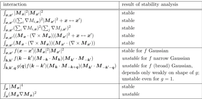
3.2.3. Stability analysis of the Ginzburg-Landau expansion . . . . 32
3.3. Blue Phases . . . . 34
3.3.1. Blue Phases in cholesteric liquid crystals . . . . 34
3.3.2. Chiral Ferromagnets . . . . 39
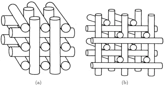
3.3.3. Single Double-Twist Cylinders . . . . 42
3.3.4. Crystal of Double Twist Cylinders I: Square Lattice . . . . 44
3.3.5. Crystal of Double Twist Cylinders II: Cubic Lattice . . . . 46
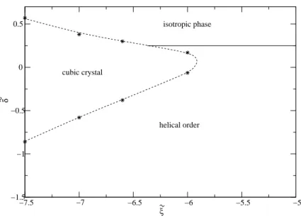
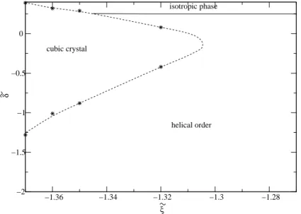
3.3.6. Phase Diagram . . . . 51
3.3.7. Blue Phases and MnSi . . . . 51
3.3.8. Other propositions for helical spin crystals . . . . 53
3.3.9. Summary and further directions . . . . 55
A. Minibands 59
A.1. Dzyaloshinsky-Moriya interaction . . . . 59
A.2. The space group P2 1 3 . . . . 60
A.3. Representations and multiplication tables for T . . . . 60
A.4. Polarization bubble: Calculations . . . . 61
B. New Phases from a Ginzburg-Landau Theory 65 B.1. Square lattice . . . . 65
B.2. Cubic lattice . . . . 66
II. Quantum Phase Transitions in Antiferromagnetic Metals 73 4. Introduction 75 4.1. Theory . . . . 75
4.1.1. Hertz-Millis theory of Quantum Critical Points in Metals . . . . 77
4.1.2. Quantum critical points in itinerant ferromagnets . . . . 79
4.1.3. Hertz-Millis theory and antiferromagnets . . . . 80
4.1.4. Other theories for heavy fermion criticality . . . . 83
4.2. Antiferromagnetic QCPs in Experiments . . . . 85
5. Field-tuned Quantum Phase Transitions 89 5.1. Model and Effective action . . . . 89
5.1.1. Magnetic insulators . . . . 93
5.2. Renormalization group equations and correlation length . . . . 94
5.3. Thermodynamic quantities . . . . 95
5.3.1. Specific heat . . . . 96
5.3.2. Magnetization, magnetocaloric effect and Gr¨ uneisen parameter . . . . 98
5.3.3. Susceptibility . . . . 101
5.4. Scattering rate . . . . 102
5.5. Discussion . . . . 104
6. Beyond Hertz-Millis Theory 107 6.1. Functional Renormalization Group . . . . 107
6.2. Model and fRG-equations . . . . 108
6.2.1. Definitions and Notation . . . . 108
6.2.2. fRG Equation for the Effective Action Γ . . . . 111
6.2.3. Choice of Cutoff Functions . . . . 113
6.3. Flow Equations for the 1-PI Vertex Functions . . . . 116
6.3.1. Approximations in the Vertex Functions . . . . 117
6.3.2. Flow for a constant Fermion-Boson Vertex . . . . 118
6.3.3. Flow Equations for the Vertex Functions . . . . 120
6.4. Summary and Outlook . . . . 126
A. Field-tuned Quantum Phase Transitions 131 A.1. Cubic terms in the effective action . . . . 131
A.2. Frustration in BEC of Magnons . . . . 131
A.3. Derivation of RG-equations . . . . 133
B. Beyond Hertz-Millis Theory 139
B.1. Bosonic self-energy Σ B . . . . 139
B.2. Fermionic self-energy Σ F . . . . 140
B.3. Fermion-boson vertex V . . . . 142
B.3.1. Fermion-boson vertex V at zero external frequencies . . . . 142
B.3.2. Fermion-boson vertex V at s F . . . . 143
B.3.3. Fully frequency-dependent V . . . . 144
B.4. Four-boson vertex Γ φ 4 . . . . 145
B.5. Continuous Hubbard–Stratonovich transformation . . . . 148
B.5.1. Field redefinition invariance of the partition sum . . . . 149
B.5.2. Method 1 . . . . 150
B.5.3. Method 2 . . . . 150
B.5.4. Method 3 . . . . 152
Bibliography 155 Danksagung 161 Anh¨ ange gem¨ aß Pr¨ ufungsordnung 163 Kurze Zusammenfassung . . . . 165
Abstract . . . . 167
Erkl¨arung . . . . 169
Teilpublikationen . . . . 169
The Fermi liquid description of metals is of paramount importance to the quantum theory of solids. First formulated by Landau in the 1950’s, the theory predicts that at very low temperatures a system of strongly interacting electrons can be described by weakly interacting electron-like “quasiparticles”. Although these quasiparticles are in fact complex many-body approximations, they have many properties in common with electrons: the quasiparticles have the same quantum numbers as electrons and the quasiparticle energy spectrum is in one-to-one correspondence with the energy spectrum of a free Fermi gas.
Starting in the early eighties, more and more materials have emerged whose experimentally observed behaviour is inconsistent with Fermi liquid phenomenology. Most notably, exponents characterizing the temperature-dependence of thermodynamic and transport quantities can deviate from those predicted by Fermi liquid theory. This “Non-Fermi liquid behaviour”
encompasses a wide range of physical phenomena, many of which are subject of current theoretical and experimental interest. For example, collective excitations of the electronic quasiparticles can dominate the low-energy behaviour of a system in the vicinity of a quantum critical point. In this case, the Fermi liquid paradigm in fact does not fail, since electronic quasiparticles are still present in the system. In other cases, however, the quasiparticle concept breaks down completely and the elementary excitations of the system are no longer of an electronic nature at all. Examples are one-dimensional metals (Luttinger liquids), where separate spin and charge degrees of freedom exist, and the fractional Quantum Hall effect, where the elementary excitations can be shown to have fractional charge.
This thesis focusses on two classes of systems that exhibit non-Fermi liquid behaviour in ex- periments. In the first part of the thesis we investigated aspects of chiral ferromagnets. In these ferromagnetic materials, the absence of inversion symmetry and the subsequent appear- ance of spin-orbit coupling gives rise to a helical modulation of the ferromagnetically ordered state. A much-studied example for this class of systems is MnSi, in which the temperature dependence of the resistivity has an exponent of 1.5 in a large section of the phase diagram.
Moreover, recent neutron scattering experiments uncovered the existence of a peculiar kind of partial order in a region of the phase diagram adjacent to the ordered state of MnSi. So far, no theoretical explanation has been found for either the non-Fermi liquid behaviour or the partial order.
In the second part of the thesis, we study aspects of quantum critical points in antiferromag-
netic metals. There are many antiferromagnetic heavy-fermion systems that can be tuned
into a regime where they exhibit non-Fermi liquid exponents in the temperature dependence
of thermodynamic quantities such as the specific heat capacity; this behaviour could be due
to a quantum critical point. Unfortunately, an extension of the Ginzburg-Landau-Wilson
theory of order-parameter fluctuations to a position- and time-dependent order parameter
for quantum critical points fails to model the experimental data of many of these systems
– a theoretical description of the observed non-Fermi liquid behaviour in such systems is an ongoing challenge.
Thesis outline
The first chapter of the first part of this thesis constitutes an introduction to MnSi: an overview of experiments as well as the current status of the theoretical description of the system is given.
In the second chapter we study the motion of electrons in a helical state by calculating the generic band-structure of electrons in the magnetically ordered state of a metal without inversion symmetry. We found that even in the case of weak spin-orbit interaction, as realized in MnSi, the answer to this question is surprisingly complex: the interplay of two weak spin- orbit effects of similar strength leads to a pronounced restructuring of the Fermi surface.
For a large portion of the Fermi surface the electron motion parallel to the helix turns out to be almost completely frozen. Signatures of this effect can be expected to show up in measurements of the anomalous Hall effect.
In the third chapter we focus on the partially ordered state of MnSi, with the underlying premise that this partially ordered state is indeed a thermodynamically distinct phase. We therefore investigated an extended Ginzburg-Landau theory for chiral ferromagnets which includes momentum-dependent interaction terms. In a certain parameter regime, we estab- lished the emergence of crystalline phases that are reminiscent of the so-called blue phases in liquid crystals. We discuss the relevance of our results to the phase diagram of MnSi. This concludes the first part of the thesis.
The second part starts with an introduction to quantum critical points with a particular emphasis on the Hertz-Millis-Moriya theory of order parameter fluctuations, its shortcomings and possible alternatives. We also give a very brief overview of the experimental status.
Many recent experiments on quantum critical points focus on field-induced quantum criti- cal behavior. A magnetic field applied to a three-dimensional antiferromagnetic metal can destroy the long-range order and thereby induce a quantum critical point. In Chapter 5, we investigated theoretically the quantum critical behavior of clean antiferromagnetic metals subject to a static, spatially uniform external magnetic field. The external field does not only suppress (or induce in some systems) antiferromagnetism but also influences the dynamics of the order parameter by inducing spin precession. We investigated how the interplay of precession and damping determines the specific heat, magnetization, magnetocaloric effect, susceptibility and scattering rates. We found that the susceptibility χ = ∂M/∂B is the ther- modynamic quantity which shows the most significant change upon approaching the quantum critical point and which gives experimental access to the (dangerously irrelevant) spin-spin interactions.
The subject of the last chapter of the thesis is the quantum critical behaviour of two-
dimensional antiferromagnetic metals. Going beyond an order parameter theory, we inves-
tigated the interaction of the electronic degrees of freedom with their collective fluctuations
by means of a functional Renormalization Group calculation. Preliminary results indicate a
behaviour of the system that is incompatible with the Hertz-Millis picture.
Metallic Magnets without Inversion
Symmetry: MnSi
The transition-metal compound MnSi has been known for more than 35 years to exhibit a helical modulation of the ferromagnetic order in its ordered phase, due to weak spin-orbit (SO) coupling. This has been predicted theoretically [1], and verified in numerous experiments [2, 3].
1.1. Experimental observations
Experimentally, MnSi is one of the best-studied metals. Its crystal structure is P2 1 3 (T 4 ), with a lattice parameter a = 4.558A ◦ . Until recently, it seemed to be a textbook example for Fermi liquid theory with a well-established magnetic phase diagram. At ambient pressure, MnSi orders around 29 K with a helical modulation of the magnetization. It exhibits an average moment of up to 0.4µ B Mn atom, where µ B is the Bohr magneton. Small external magnetic fields of about 0.12 T reorient the helix parallel to the field, and magnetic fields above 0.62 T destroy the helical order: the system becomes ferromagnetic [4].
While the physics of the ordered phase has been well understood for almost 25 years, the interest in MnSi was recently renewed [5, 6, 7] after it was discovered [5] that moderate pressures p suppress the long range helical order and drive the system for p > p c ≈ 14.6 kbar into a novel state (see Fig. 1.1). In this state, the system is characterized by an anomalous resistivity, ρ ∼ T 3/2 , which is incompatible with Fermi liquid theory. This behaviour is observed over almost three decades [5] in temperature T and over a huge pressure range [6].
Lattice constants remain essentially unchanged throughout the pressure change.
Novel metallic phases have been postulated for a number of systems, notably in high-tempera-
ture superconductors and heavy fermion compounds. In most of these cases, the existence
of such phases is highly controversial, for various reasons: fine-tuning of the experimental
conditions is often necessary, the crystal structures contain defects, and characteristic energy
scales are of similar magnitude and cannot be separated properly. In MnSi, however, the
region of the phase diagram where anomalous resistivity behaviour is observed is so large
that fine-tuning is unnecessary. Moreover, MnSi can be produced at high purity and high
crystal perfection with a mean free path of 5000A ◦ and a residual resisitivity of 0.17µΩ. Finally,
the three most relevant energy and length scales are well separated: first, there is itinerant
ferromagnetism on length scales of a few lattice constants, second, weak spin-orbit interaction
induces the helical modulation of the ferromagnetic order with a pitch of 170A ◦ at ambient
pressure, and third, spin-orbit coupling terms of higher order lock the direction of the helix to
q 0 = h 111 i . The typical size of magnetic domains in the ordered state is 10 4 A ◦ . The resistivity
data on MnSi has therefore been taken as evidence for the existence of a genuine non-Fermi
liquid phase.
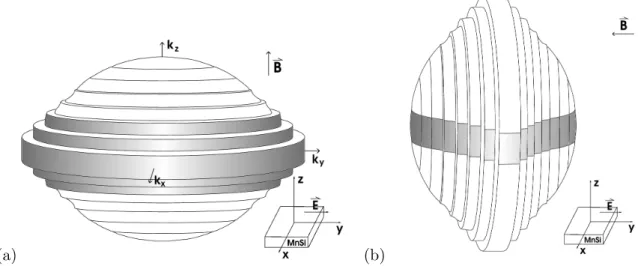
(a) (b)
Figure 1.1.: (a) Temperature T versus pressure p phase diagram of MnSi. In the partially ordered phase, the exponent describing the temperature dependence of the elec- trical resistivity, α, changes apruptly from 2 to 1.5. The non-Fermi liquid phase extens at least up to 30 kbar and down to temperatures of 20 mK. The transition described by T c changes from second order to first order as T c drops below ∼ 12 K. Taken from [8](b) Distribution of the magnetic scattering intensity for heli- cal magnetic order observed at ambient pressure (left sphere) and for the partial magnetic order observed for p > p c (right sphere). Taken from [7].
Recent neutron scattering results [7] for p > p c give tantalizing hints as to the origin of this non-Fermi liquid phase: they suggest that while true long-range order is lost in this phase, a peculiar partial helical order survives on intermediate time and length scales.
In the ordered phase, elastic neutron scattering experiments confirm the existence of long- range helical ordering of the magnetization: at ambient pressure, resolution-limited Bragg peaks are observed at q 0 = h 111 i and | q 0 | = 0.037A ◦ −1 , corresponding to the helix wave vector.
In the vicinity of the ordered phase but still within the non-Fermi liquid phase there is a region where neutron scattering shows signs of static magnetic order (see Fig. 1.1), although bulk properties suggest the loss of long-range order at p c . More precisely, the scattering intensity is now peaked on the surface of a sphere with a radius equal to the helical wave vector | q 0 | = 0.043A ◦ − 1 : scans radial to that sphere show resolution-limited peaks, whereas tangential scans show a broad angular spread of the signal. There is almost no signal left in the h 111 i -directions, the intensity is now peaked around h 110 i instead. The integrated scattering intensity over that sphere is comparable in magnitude to the scattering intensity at ambient pressure. This signal is lost above a crossover temperature T 0 .
Recent experiments in magnetic fields further corroborate the existence of this partially or-
dered state, see Fig. 1.2: When tuning from the partially ordered state through the helical
phase into the ferromagnetic phase with a magnetic field, a hysteresis loop for the intensity
of the Bragg peak at q 0 = 0.04A ◦ − 1 can be observed. The intensity reaches its peak in the
helical phase, but goes down as the field is lowered once again, indicating that the helical
order is partially destroyed. Even for zero magnetic field, however, the intensity does not go
back down to zero; some kind of order remains.
(a) (b)
Figure 1.2.: (a) Temperature T versus magnetic field B phase diagram of MnSi for a pressure p = 15.50 kbar about 1 kbar above the critical pressure. The magnetic state changes from partially ordered to long-range helical order at H m and becomes ferromagnetically ordered above H c2 . Taken from [8]. (b) Field dependence of the intensity of the Bragg peak at q 0 = 0.04A ◦ −1 on a small angle scattering instrument. For high fields, helical order is destroyed and ferromagnetic order is induced. Taken from [9].
NMR-measurements complement this picture: recent data [10] support the existence of static or slowly fluctuating magnetism well above the critical pressure p c . These results are partic- ularly interesting because NMR measurements probe much longer time scales than neutron scattering experiments.
What are other signatures of (i) the first order transition between the helical and the NFL phase (ii) the crossover line T 0 e.g. in thermodynamic and transport quantities? There is a sharp drop in the residual electrical resistivity at T c , but no signatures are seen at T 0 . The a.c. susceptibility is equally unaffected at T 0 .
There are a large number of materials with the same crystal structure as MnSi, e.g. FeSi and CoSi. Although FeSi is a narrow-gap semiconductor and CoSi is a diamagnetic semimetal, the doped material Fe x Co 1 − x Si is a metal with helical spin structure in the concentration range 0.2 < x < 0.95. The pitch of the helix in Fe x Co 1 − x Si is even larger than in MnSi (e.g. 295A ◦ and 430A ◦ for x=0.8 and 0.9 respectively). In a recent publication [11], the helical spin order in Fe 0.5 Co 0.5 Si has been observed in real space by means of Lorentz transmission electron microscopy. The images reveal a surprising number of helical magnetic defects in the form of dislocations and domains with diffuse boundaries, which were not strongly pinned by atomic defects and could be reoriented with an external magnetic field.
Finally, anomalous behaviour of the resistivity at low temperatures is observed in a number of ferromagnets, notably ZrZn 2 [12], UGe 2 [13], UCoAl [14], CoS 2 [15] as well as Ni 3 Al and YNi 3 [16]. At very low temperatures, these materials exhibit a temperature dependence of the resistivity of the form ρ ∼ a + b T α , with α well below 2. Moreover, this behaviour is not always restricted to very low temperatures and a rather narrow pressure range [16], as one would expect if a quantum critical point is at the origin of the anomalous exponents.
Therefore, there is a distinct possibility that the non-Fermi liquid behaviour observed in
MnSi is not due to its lack of inversion symmetry and helical twist at all. On the other hand, the ubiquitousness of non-Fermi liquid behaviour near ferromagnetic instabilities has led to speculation whether the ferromagnetic phase of some of the materials listed above is not in fact a long pitch spiral phase instead.
1.2. Theory
Little is known from the theoretical side either on the nature of the partially ordered state or on the non-Fermi liquid behaviour observed. A number of scenarios have been proposed to explain the neutron scattering data; among these are the formation of metastable droplets [6], slowly meandering spirals or multi-domain states where the direction of the spiral varies strongly from one domain to the next [7]. Belitz, Kirkpatrick and Rosch considered a theory for the Goldstone modes in the ordered phase of a helical magnet [17, 18, 19]. The scattering of the electrons off these Goldstone modes could then be of relevance to the non-Fermi liquid behaviour seen in MnSi if the partially ordered state consists of domains that are large enough for the electrons to interact with the Goldstone modes before they can scatter off domain walls. This scattering mechanism, however, leads to a T 5/2 -dependence of the resistivity, which means that it is an unlikely candidate to explain the non-Fermi liquid behaviour found in MnSi.
There are two theoretical predictions for the transition between the partially ordered and the isotropic phase, i.e. the T 0 -line: Schmalian and Turlakov [20] interpret the T 0 -line as the continuation of the (2nd order) phase boundary between the helical and the disordered phase;
Tewari et al. have proposed a liquid-gas transition model to be relevant for the T 0 -line in the phase diagram of MnSi [21].
Recent, more general work of relevance to MnSi includes the investigation of quantum phase
transitions of itinerant helimagnets by Vojta and Sknepnek [22], and finally, Belitz et al. have
proposed to explain the change of the transition line T c from second order to first order
behaviour to a tricritical point [23].
In the following we calculate the band structure of electrons within the magnetically ordered phase of a chiral ferromagnet and discuss its experimental consequences. In a first step, we neglect all spin-orbit effects besides the Dzyaloshinsky-Moriya interaction and show that in this case, the mini-bands, which formally arise in the reduced Brillouin zone of the helical phase, can be avoided by a specific choice of reference frame. In a second step, we take the leading spin-orbit corrections in the band-structure into account, which then drastically modify this picture: not only do minibands develop in a region of the Fermi surface, but this region is comparatively large and the minibands are exponentially flat. We discuss several experimental consequences of our results as well as the feedback of this peculiar shape of the Fermi surface on Goldstone modes in the ordered phase. Most of the work presented in this chapter has been published in [24].
2.1. Band structure from coupling of the electrons to the helix
A Ginzburg-Landau theory of magnetic systems like MnSi which lack an inversion symmetry was investigated as early as 1980 by Nakanishi et al. and Bak and Høgh [2]. The cubic metal MnSi is characterized by the space group P2 1 3 whose point group T consists only of cyclic permutations of ˆ x, ˆ y and ˆ z, of rotations by π around the coordinate axes and of combinations thereof. (The transformations contained in P2 1 3 as well as the irreducible representation of the corresponding point group are given in Appendix A.2.) Spin orbit coupling is very weak in this system and the strength of spin-orbit coupling defined below can therefore be used as a small parameter. Spin-orbit coupling manifests itself in a Ginzburg-Landau expansion of the order parameter in the form of the Dzyaloshinsky-Moriya interaction
q 0 Z
Φ (x) · ( ∇ × Φ (x)), (2.1)
where Φ is the magnetization of the system, and the prefactor q 0 is of the order of the spin-orbit coupling strength. The term (2.1) arises in the absence of inversion symmetries in linear order of spin orbit coupling; for a more detailed motivation of (2.1) see Chapter A of the appendix. As (2.1) is linear in momentum, a ground state with a finite wave vector is energetically favourable. In this case, an arbitrary small q 0 destabilizes the ferromagnetic state, twisting it into a helix of the form
Φ (x) = Φ 0 ( ˆ n 1 cos q 0 x + ˆ n 2 sin q 0 x) (2.2)
= Φ 0 2
( ˆ n 1 − iˆ n 2 )e iq 0 x + ( ˆ n 1 + i n ˆ 2 )e − iq 0 x
q 0 n 2
n 1
Figure 2.1.: Helical modulation of the magnetization. The direction of the magnetization twists around the q 0 -axis, planes of constant magnetization are perpendicular to q 0 .
where ˆ n 1 ⊥ n ˆ 2 ⊥ q 0 are three perpendicular vectors and | q 0 | = q 0 . A more thorough discussion of the Ginzburg-Landau theory of a chiral ferromagnet will be presented in the following chapter. Since relativistic effects are weak, the pitch 2π/q 0 of the helix should in general be large: it is 175A ◦ in the case of MnSi and even larger (> 300 A ◦ ) in the case of the isostructural compound Fe x Co 1−x Si. The dimensionless constant δ DM = q 0 /k F , where k F is a typical Fermi momentum, is therefore at most of the order of a few percent. The energy gain due to the formation of the helix is of order δ 2 DM , as can be seen from Eq. (2.1): when the helix solution (2.2) is inserted into (2.1), both the prefactor and the helix wavevector contribute a factor of δ DM . Higher order corrections of order δ DM 4 can be shown to lock the direction of the helix to the h 111 i direction if q 0 is negative, which is the case for MnSi, or to the h 100 i direction for positive q 0 [2]. While these terms are important for the Goldstone modes in the system [17], they can be neglected for the following discussion.
The large pitch of the helix implies a large unit-cell in the ordered phase with more than 300 atoms which makes a band-structure calculation from first principles difficult. So far, only non-relativistic calculations [25, 26] exist; those assume a ferromagnetic state and neglect the helical modulation. The results are rather complex with several bands crossing the Fermi energy, which is consistent with de Haas-van Alphen experiments [26] in large magnetic fields.
We will not try to model these details: for example, we will not keep track of multiple bands.
Instead, we want to capture the main qualitative features in the band-structure, and we therefore consider the following simple non-interacting one-band Hamiltonian
H 0 = X
k,αα ′
ǫ αα k ′ c † kα c kα ′ + 2 Z
d 3 x Φ (x)S(x) (2.3)
where S(x) = P
e i(k − k ′ )x c † kα σ αα ′ /2 c k ′ α ′ is the spin of the conduction electrons and Φ (x) is defined in Eq. (2.2). Note that (2.3) is already strongly simplified: in real systems ǫ αα k ′ can depend on the magnetization and interband couplings may be relevant for a quantitative description, but we will neglect these aspects in the following calculation.
In a first step, we disperse with spin-orbit effects in the band-structure, assuming that ǫ αα k ′ =
ǫ 0 k δ αα ′ . While we will show below that this approximation turns out to be unjustified, it will
serve as a starting point for the full calculation.
The coupling of the electrons to the helical ordered state Φ , i.e. the second term of (2.3), formally leads to a coupling of electrons with different wave vectors, since
2 Z
d 3 x Φ (x)S(x) = Φ 0
Z
d 3 x X
e i(k − k ′ )x
c † k ↑ e − iq 0 x c k ′ ↓ + c † k ↓ e iq 0 x c k ′ ↑
. (2.4)
However, for the case of a spin-rotation invariant band-structure, a residual symmetry leads to a very simple band-structure. In the magnetically ordered state, the helical modulation breaks spontaneously both the spin-rotation invariance and the translational invariance along q 0 . Nonetheless, the product of a translation by a lattice vector x and a rotation of spins around the q 0 axis by an angle − q 0 x
T ˜ x = e ixP e − iq 0 x R d 3 x ′ (S(x ′ )q 0 )/q 0 (2.5) is still a symmetry of the Hamiltonian, where P is the generator of translations. As a consequence, instead of many minibands (in a reduced Brillouin zone of width q 0 ) just two bands form like in the ferromagnetic state. This can be seen by going to a frame of reference rotating with the helix, i.e. by applying the unitary transformation U with
U = e i R d 3 x q 0 z S z (x) = e 2 i R d 3 x q 0 z c † α (x)σ z αα ′ c α ′ (x) , (2.6) where we assumed ˆ z k q 0 for notational simplicity, so that the electrons are transformed as
c k,σ → U + c k,σ U = Z
d 3 x e i kx
e − iq 0 z σz 2
σσ ′ c σ ′ (x) = c (k − σq 0 /2),σ . (2.7) In this coordinate system, Φ(x) = Φ 0 x ˆ is a constant vector pointing into the ˆ x direction and the Hamiltonian (2.3) takes the form
H 0 = X
k
c † k, ↑ c † k, ↓ ǫ 0 k+ q 0 2
Φ 0
Φ 0 ǫ 0 k
− q 2 0
! c k, ↑ c k,↓
(2.8)
and the 2 × 2 matrix can now easily be diagonalized to calculate the dispersion:
E ± (k) =
ǫ 0 k+ q 0 2
+ ǫ 0 k
− q 2 0
2 ±
v u u t
ǫ 0 k+ q 0 2 − ǫ 0 k
− q 2 0
2
4 + Φ 2 0 ≈ ǫ 0 k ± Φ 0 ± (v k q 0 ) 2
8 | Φ 0 | (2.9)
where we used that q 0 is small. In this rotated frame, one obtains the Fermi surface of a ferromagnetic state: the two bands are essentially separated by 2Φ 0 , with a slight deformation in the q 0 direction caused by the last term of (2.9). As emphasized above, no minibands form. The eigenstates d k, ± in which H 0 = P
i= ± E i (k)d † ki d ki is diagonal are given by d k, ± =
± 1/ √
2(c k,↑ ± c k,↓ ) to lowest order in spin-orbit coupling. The main results of this chapter
have been published in [24].
2.2. Form of the spin-orbit coupling term in the bandstructure
We want to derive the most simple form that spin-orbit coupling can take in the bandstructure of the electrons while respecting the crystal symmetry. The crystal lattice of MnSi is invariant under transformations of the space group P 2 1 3 (T 4 ). The lack of inversion symmetry of this crystal lattice is a necessary prerequisite for spin-orbit coupling in the bandstructure: in the presence of inversion symmetry,
E k ↑ T−reversal = E − ↓ k inversion = E k ↓ , (2.10)
and spin-orbit coupling terms are absent. In general, spin-orbit coupling is included in the Hamiltonian via a term of the form
H soc ∝ σ · (k × E), (2.11)
where E is the electric field induced by the crystal potential. This term is of relativistic origin; its prefactor is small.
Let us treat spin-orbit coupling as a perturbation and consider how crystal symmetry restricts the form of the spin-orbit coupling correction of first order in δ to the Hamiltonian at a general point k in the Brillouin zone without band degeneracy and for one specific band, neglecting interband mixing.
What kind of spin-orbit corrections in the band structure of the electrons are compatible with the symmetry group? The general ansatz for spin-orbit coupling terms in the Hamiltonian is
H soc = g k · σ, (2.12)
where g k = (g x k , g k y , g z k ). The possible form of g k in (2.11) is restricted by the requirement that the representation of the space group of the crystal according to which H soc transforms has to contain the identity representation. A list of the irreducible representations of T (i.e. the point group of P2 1 3) is given in Appendix A.3. The irreducible representation according to which σ transforms has to be F , since T has only one three dimensional irreducible representation.
As a consequence, g k has to transform according to F as well. When g k is expanded in momenta, the lowest order term is simply
g k = k, (2.13)
since k x , k y , k z are basis functions for F in k-space (see [27], erratum).
2.3. Electron band structure and the Fermi surface
Spin-orbit coupling terms in the band structure occur to first order in spin-orbit coupling and therefore to the same order in spin-orbit coupling as the Dzyaloshinskii-Moriya interaction – it is a priori not clear why they should be neglected. As discussed in section 2.1, we therefore set ǫ αα k ′ = ǫ 0 k δ αα ′ + P
g k i σ αα i ′ where g k ∝ k. As g k arises to first order in the spin-orbit
coupling, typical matrix elements are of order δ B ǫ F , where ǫ F is the Fermi energy and the dimensionless constant δ B has the same order of magnitude as δ DM
δ B ∼ δ DM = q 0 /k F ∼ δ (2.14)
and is therefore small, i.e. of the order of a few percent in MnSi. We will continue to use δ B as well as δ DM to make the origin of different contributions to the Hamiltonian of the system more apparent. The full Hamiltonian H is given by
H = H 0 + H SO = H 0 + X
k
g i k σ i αα ′ c † kα c kα ′ (2.15)
with H 0 from (2.3). Throughout the rest of this chapter we will set the ˆ z-axis parallel to the helix wave vector q 0 .
To extract the main effect of H SO on the band structure discussed in section 2.1, a sequence of transformations will be performed on H:
(1) Even though spin-orbit coupling terms break the residual symmetry (2.5) in real systems, it is convenient to transform H SO first to the rotating frame, where
H SO ≈ X
k
c † k − q
0 /2, ↑
c † k+q
0 /2, ↓
! T
g z k g k x − ig k y g x k + ig k y − g k z
c k − q
0 /2, ↑
c k+q 0 /2, ↓
, (2.16)
and then to the eigenstates d k, ± corresponding to the energies E ± (k) in Eq. (2.9) ,
H SO ≈ 1 2
X
k
d † k − q
0 /2,+ − d † k − q
0 /2, −
d † k+q
0 /2,+ + d † k+q
0 /2,−
! T
g z k g x k − ig k y g x k + ig y k − g k z
d k − q 0 /2,+ − d k − q 0 /2, − d k+q 0 /2,+ + d k+q 0 /2, −
. (2.17) In this basis, H 0 is diagonal, and all off-diagonal matrix elements are at least of order δ B and therefore small.
(2) H SO induces transitions from k to k + q 0 and leads to the formation of mini-bands in the new Brillouin zone of width q 0 . As the + and − band of H 0 are separated by Φ 0 ≪ q 0 , transitions between these bands in the presence of H SO can be neglected, and H can be separated into two contributions H SO + and H SO − :
H SO − = X
E − (k)d † k − d k − − X d † k − q
0 /2, −
g k x − ig y k
2 d k+q 0 /2, − + h.c.
(2.18) H SO + = X
E + (k)d † k+ d k+ + X d † k − q
0 /2,+
g x k − ig y k
2 d k+q 0 /2,+ + h.c. (2.19)
The contributions due to g z only lead to a minor deformation of the bands and can therefore
be absorbed in E ± . We will restrict the following discussion to H SO − ; analogous contributions
can be expected from H SO + as well. Although the second term of H SO − is linear in spin-orbit
coupling, it is not always small compared to the first term: for regions on the Fermi surface
where E − (k) − E − (k + q 0 ) is very small, it is the second term that dominates and gives rise to non-negligible corrections to the band-structure.
(3) To take a closer look at the region where E − (k) − E − (k + q 0 ) ≪ 1, where the main effects from spin-orbit coupling terms in the band structure can be expected to arise, we expand E − (k) around planes in momentum space where the Fermi velocity ∂ k E − (k) is perpendicular to Q 0 and account for the band structure in the magnetic Brillouin zone of width q 0 in the ˆ
z-direction by introducing new momentum coordinates (κ ⊥ , κ z , n), where n is an integer (the band index) and − q 0 /2 < κ z < q 0 /2 is a momentum in the reduced Brillouin zone. By construction, k z = k 0 z + κ z + nq 0 and ∂ k E − (κ ⊥ , k z 0 )q 0 = 0. In this region,
E − (κ ⊥ , κ z , n) ≈ E − (κ ⊥ ) + (κ z + nq 0 ) 2 /(2m κ ⊥ ) (2.20)
g k x − ig k y ≈ const. (2.21)
where m κ ⊥ is a measure of the curvature of the Fermi surface. For fixed κ ⊥ and k z the Hamiltonian (2.18) takes the form
H SO κ ⊥ ,κ z ≈ ǫ F
X
n
c 1 δ B (d † n+1 d n + d † n d n+1 ) + c 2 δ DM 2 (n − κ z
q 0 ) 2 d † n d n + c 3 (2.22) where c 1 = | g x k
⊥ ,k z 0 − ig y k
⊥ ,k 0 z | /(2δ B ǫ F ), c 2 = k F 2 /(2m κ ⊥ ǫ F ) and c 3 = E − (κ ⊥ , k z 0 )/ǫ F are con- stants of order 1. The special case where c 1 vanishes at some points on the Fermi surface, i.e. where | g k × q 0 | = 0, will be discussed below. For finite c 1 , interband coupling takes the form of a tight binding Hamiltionian. The band-structure (2.9) was due to the second term in Eq. (2.22), which contributes only to order δ 2 DM ∼ δ 2 B . The first term, which originates from g k x − ig k y , is linear in spin-orbit coupling and can therefore be expected to strongly modify (2.9). The qualitative aspects of the spectrum of the Hamiltonian (2.22) can now already be read off by comparing Eq. (2.22) to the Hamiltonian of a harmonic oscillator.
(4) For a more detailed analysis of the spectrum of (2.22) it is convenient to Fourier transform it from band-index space n to the conjugate variable ξ. Setting
d n = X
e − inξ d ξ , d † n = X
e inξ d † ξ , (2.23)
the Hamiltonian (2.22) reads (in first quantized notation) H SO κ ⊥ ,κ z ≈ ǫ F
"
2c 1 δ B cos(ξ) − c 2 δ 2 DM
∂ ξ + i κ z q 0
2
+ c 3
#
. (2.24)
The dependence of (2.24) on κ z can be absorbed in the boundary condition by a gauge transformation Ψ → e iξκ z /q 0 Ψ, so that we finally have
H SO κ ⊥ ≈ ǫ F
2c 1 δ B cos(ξ) − c 2 δ DM 2 ∂ ξ 2 + c 3
. (2.25)
The fact that the κ z -dependence of (2.24) can be eliminated by a gauge transformation also
shows that the spectrum of (2.25) is the same as for (2.22) with varying κ z , or, in other words,
that the bandwidth of (2.22) in the q 0 -direction is the same as the bandwidth of (2.25). (2.25)
is now the familiar Hamiltonian of a particle in a periodic potential. Similar models show up
in many different problems, see e.g. ref. [28] where eigenfunctions of (2.22) are discussed in
detail.
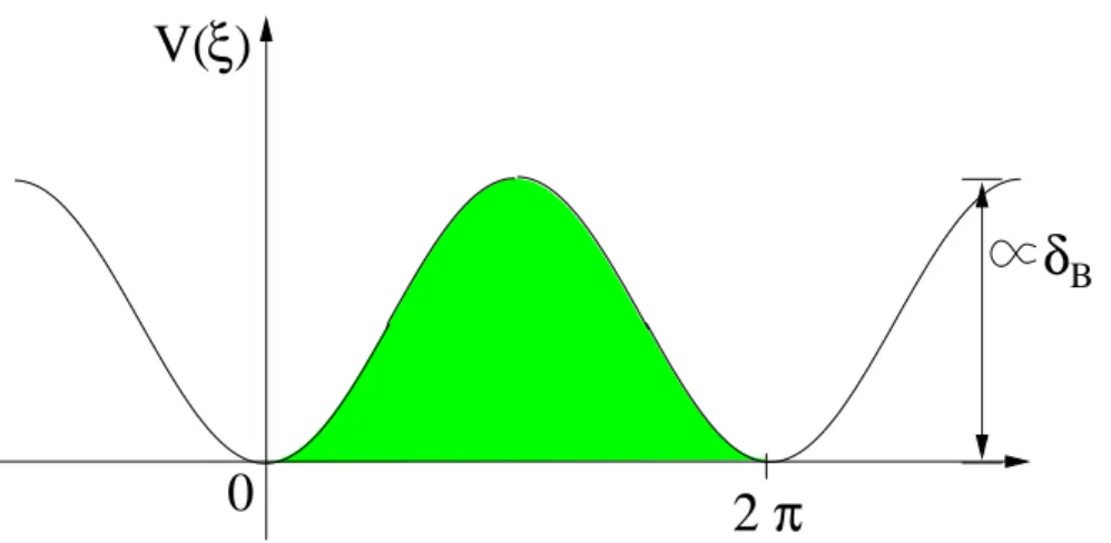
δ B ξ
V( )
0 2 π
Figure 2.2.: The cosine potential of (2.25). For energies much larger than the peak height, particle motion is not affected by the potential. For very low energies, the particle oscillates around a potential minimum. The instanton energy is equal to the energy needed to cross the barrier, i.e. to the shaded area.
2.3.1. Band structure
Since the cosine potential, i.e. the first term of (2.25), is proportional to δ B , this term originates from H SO in contrast to the second term which arises as a consequence of the Dzyaloshinsky-Moriya interaction term in the original Hamiltonian. Whether H SO modifies the spectrum (2.9) or not depends on how strong the influence of the cosine potential is, and therefore the spectrum of (2.25) can be easily obtained in two limits.
For energies E ≫ E 0 = ǫ F δ B much higher than the cosine potential, the periodic potential has little influence. The dispersion relation (2.9) is recovered, and the bandgaps at the boundaries of the magnetic Brillouin zone are exponentially small and are therefore irrelevant.
In the other limit E ≪ E 0 , the “particle” sits deep in the minima of the cosine potential.
In this limit, the potential can be approximated to great accuracy by a harmonic oscillator potential, and the band-splitting, or rather the level spacing ∆E, can be directly read off from the prefactors of the terms in (2.25): Setting ε F c 2 δ DM 2 = 1/(2m) and ε F c 1 δ B = mω 0 2 /2, where m is the mass of the harmonic oscillator and ω 0 its frequency,
∆E = ω 0 = 2ǫ F δ DM p δ B √
c 1 c 2 ∝ δ 3/2 . (2.26)
The harmonic oscillator levels are slightly broadened by tunnelling events, when the particle tunnels from one minimum of the cosine potential to the next. This gives a finite bandwidth W , which can be calculated with the help of a WKB approximation or an instanton expansion:
W ∼ ∆E e − S 0 , (2.27)
(see [29], chapter 7), where S 0 is the energy of one instanton, i.e. the energy needed by the particle to tunnel from one minimum of the cosine potential to the next,
S 0 = Z 2π
0
dξ √
2mV = Z 2π
0
dξ
s 2c 1 δ B
c 2 δ DM 2 (cos ξ + 1) = 8 √ 2
r c 1 c 2
√ δ B
δ DM ∝ δ − 1/2 , (2.28)
E
k
2 q 0
− + 2 q 0
z
Figure 2.3.: Band structure of the Hamiltonian (2.3) with ǫ 0 k = k 2 /2 − 1/2, Φ 0 = 0.3, q 0 = (0, 0, 0.1), g k = 0.1k, k x = 1.26, k y = 0 which corresponds to δ DM = δ B = 0.1, c 1 ≈ 1.26, c 2 ≈ 1. The lowest bands have exponentially small band widths, e.g.
2 · 10 −10 ǫ F for the first band, consistent with Eq. (2.29). Only the E − bands are shown.
and therefore W ∼ ∆E exp
"
− 8 r c 1
c 2
√ δ B δ DM
#
∼ δ 3/2 exp
− c ′ 1
√ δ
. (2.29)
And finally, the number of bands that are exponentially flat can be estimated by counting the number of bands n max whose energy is smaller than E 0 :
n max ∼ E 0
∆E ∼
√ δ B
δ DM ∼ δ −1/2 . (2.30)
To sum up, the interplay of the Dzyaloshinsky-Moriya interaction of strength δ DM and spin- orbit coupling in the band-structure parameterized by δ B , two weak relativistic effects, leads to the formation of exponentially flat bands. In those bands, the motion of the electrons parallel to the wave vector q 0 of the helix practically stops. The non-analytic dependence of W and ∆E on δ B and δ DM shows that this is a non-perturbative effect, which originates from the interplay of resonant backscattering from the helix and crystal field effects. Corrections to the exponent in (2.29) are of the order (n + 1/2) 2 δ DM / √
δ B , where n is the band index.
We have confirmed our analytical results (2.26), (2.29) and (2.30) by comparing to a numerical diagonalization of the Hamiltonian (2.3) shown in Fig. 2.3. Note that the transition from equidistant harmonic oscillator bands to bands with negligible bandgaps, i.e. the transition between the two limiting cases, happens quite abruptly over the distance of roughly two bands.
2.3.2. Shape of the Fermi surface
In which way does the band structure found in the previous section affect the shape of the
Fermi surface? Let us consider the Fermi surface in the extended Brillouin zone, where
k = (κ ⊥ , k z ). For ε 0 k = k 2 /2m quadratic in k and for δ B = 0, there are two ellipsoidal Fermi surfaces, which are given by
0 = E ± (κ ⊥ , k z ) − E F = κ 2 ⊥
2m + k 2 z + (q 0 /2) 2
2m ±
s q 0 k z 2m
2
+ Φ 2 0 − E F , (2.31)
where E F is the Fermi energy. For δ B 6 = 0, the κ ⊥ - and k z -dependent parts of the energy are still independent of each other, i.e.
E(κ ⊥ , k z ) = κ 2 ⊥
2m + f (k z ), (2.32)
where f(k z ) now describes minibands close to ∂ k E(k) · q 0 = 0. The κ ⊥ -dependent part of (2.32) serves to shift the Fermi level through the energy levels of H (see Fig. 2.3) and thus transfers the band structure of H to the Fermi surface. The resulting Fermi surface (for one band only) is shown in figure 2.4.
The interplay of the two spin-orbit coupling terms present in the model causes a whole section of the Fermi surface to split up into bands with negligible bandwidth and huge band gaps in between. Electrons from that belt-shaped region of the Fermi surface will stop their motion parallel to q 0 . The width w of the belt of minibands can be estimated from (2.30) as follows:
there are n max minibands of width q 0 , and therefore w ∼ k F δ DM
√ δ B
δ DM = k F p
δ B . (2.33)
As a result, even for very small δ B of the order of a few percent, a sizable fraction of the Fermi surface is affected by those ultra-flat bands. It is interesting to note that the belt of minibands perseveres even if δ B is small compared to δ DM . In the limit δ B → 0 and δ DM = const. the bandgaps do not close, but instead the section of the Fermi surface containing the mini-bands gets smaller until it eventually vanishes. Even when δ B is small, mini-bands are present in principle, although only in a small region on the Fermi surface.
If | g k × q 0 | = 0 at some singular points on the Fermi surface in the vicinity of the region where q 0 is parallel to the Fermi surface, the results quoted above are not valid close to those points. In this case, g k x
⊥ ,k 0 z − ig y k
⊥ ,k 0 z can be approximately linearized, and the first term in eq. (2.22) has to be replaced by ǫ F P
n c ′ 1 δ DM δ B (d † n+1 d n + d † n d n+1 )(n − κ z /q 0 ). This term is now of order δ 2 and will generate O (δ B /δ DM ) ≈ 1 minibands that will cover an area of width k F δ B close to these points.
2.4. Fermi surface: Experimental consequences
The interplay of the two spin-orbit coupling effects in the model leads to the opening of large
gaps on a considerable part of the Fermi surface. In this section we want to investigate what
characteristic signatures these band gaps show either directly in experiments that probe the
Fermi surface or indirectly by affecting e.g. transport coefficients.
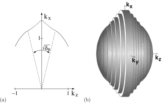
(a)
−1 1
1
k z
k x
δ B
(b)
Figure 2.4.: a) Fermi surface of the Hamiltonian (2.3) for k y = 0 in an extended Brillouin zone (ǫ 0 k = k 2 /2 − 1/2, Φ 0 = 0.3, q 0 = (0, 0, 0.1), g k = 0.1k, k x = 1.26, k y = 0 which corresponds to δ DM = δ B = 0.1, c 1 ≈ 1.26, c 2 ≈ 1). b) Sketch of the Fermi surface. In a belt of width √
δ B the mini-bands are completely flat in the direction parallel to the helix.
There are numerous experimental methods available to determine the shape of the Fermi surface of a metal; however, most of them involve the application of external magnetic fields.
The experimental difficulty in this case lies in the fact that MnSi cannot be subjected to high magnetic fields since fields larger than 0.62T destroy the helical spin ordering in the metal [4].
2.4.1. De-Haas–van-Alphen Effect
When an external magnetic field B is applied to a metal, the magnetic susceptibility can be shown to depend periodically on 1/B; this is the De-Haas–van-Alphen effect. The period of the oscillations is proportional to the extremal cross-sectional area of the Fermi surface in a plane normal to the magnetic field and therefore gives direct information on the shape of the Fermi surface.
The De-Haas–van-Alphen effect can be derived theoretically from the semiclassical equations that govern the motion of the electrons in the presence of a uniform magnetic field:
~ k ˙ = − eB × k, (2.34)
˙
r = v(k) = 1
~
∂ǫ(k)
∂k . (2.35)
The external magnetic field forces the electrons to move in the plane normal to the external
magnetic field, or more specifically, along paths formed by the intersection of the Fermi surface
00000000000 00000000000 00000000000 00000000000 00000000000 11111111111 11111111111 11111111111 11111111111 11111111111