Critical point in the QCD phase diagram for extremely strong background magnetic fields

JHEP07(2015)173

Published for SISSA by Springer

Received:May 13, 2015 Accepted: July 8, 2015 Published: July 31, 2015

Critical point in the QCD phase diagram for extremely strong background magnetic fields

Gergely Endr¨odi

Institute for Theoretical Physics, Universit¨at Regensburg, D-93040 Regensburg, Germany

E-mail: gergely.endrodi@physik.uni-r.de

Abstract: Lattice simulations have demonstrated that a background (electro)magnetic field reduces the chiral/deconfinement transition temperature of quantum chromodynam- ics for eB < 1 GeV². On the level of observables, this reduction manifests itself in an enhancement of the Polyakov loop and in a suppression of the light quark condensates (inverse magnetic catalysis) in the transition region. In this paper, we report on lattice simulations of 1 + 1 + 1-flavor QCD at an unprecedentedly high value of the magnetic field eB = 3.25 GeV². Based on the behavior of various observables, it is shown that even at this extremely strong field, inverse magnetic catalysis prevails and the transition, albeit becoming sharper, remains an analytic crossover. In addition, we develop an algorithm to directly simulate the asymptotically strong magnetic field limit of QCD. We find strong evidence for a first-order deconfinement phase transition in this limiting theory, implying the presence of a critical point in the QCD phase diagram. Based on the available lattice data, we estimate the location of the critical point.

Keywords: Lattice QCD, Lattice Gauge Field Theories, Lattice Quantum Field Theory, Phase Diagram of QCD

ArXiv ePrint: 1504.08280

JHEP07(2015)173

Contents

1 Introduction 1

2 Setup and observables 3

3 Results at eB = 3.25 GeV² 5

4 Results in the asymptotic magnetic field limit 9

5 Conclusions 14

A Effective action in the asymptotic magnetic field limit 16 B Simulating anisotropic pure gauge theory on the lattice 19

1 Introduction

Quantum chromodynamics (QCD) exhibits a finite temperature transition separating the chirally broken, low-temperature phase from the chirally symmetric, high-temperature regime, where quarks and gluons are deconfined. Although this transition is no real phase transition but merely an analytic crossover [1, 2], it is marked by the pronounced be- havior of the corresponding (approximate) order parameters: the drop in the light quark condensates, accompanied by the increase in the Polyakov loop. The characteristic de- pendence of the transition temperature on further parameters of the system probes our understanding of QCD and maps out the phase diagram in the corresponding parameter space. One parameter that is thought to have rich physical applications, ranging from neutron star physics through heavy-ion collisions to the cosmology of the early universe, is a background (electro)magnetic field B. The relevant range of magnetic fields, where QCD interactions compete with the electromagnetic forces, is given by multiples of the pion mass squaredm²_π. We refer the reader to recent reviews on the subject [3–5].

QCD with background magnetic fields can be studied directly using non-perturbative lattice simulations. Continuum extrapolated results employing staggered quarks with phys- ical masses have been used to map out the phase diagram [6] for 0≤eB <1 GeV². Accord- ing to these results, the magnetic field increases the light quark condensates well below and well above Tc (magnetic catalysis) but decreases them in the transition region [7] (inverse magnetic catalysis). As a result of this non-monotonous dependence of the condensate on B and on T, the transition temperature is significantly reduced by the magnetic field.

The same tendency has been observed for the Polyakov loop as well, giving a similarly decreasing transition temperature [8]. More recent lattice simulations employing different quark discretizations are consistent with this picture [9].

JHEP07(2015)173

The magnetic catalysis of the condensate at low temperatures is a very robust concept.

It arises naturally due to the Landau-level structure of charged particle energies in the presence of B. In the strong field limit, magnetic catalysis can be understood in terms of the dimensional reduction of the system and the high degeneracy of the lowest Landau- level [10, 11]. For low magnetic fields, it can be related to the positivity of the QED β- function that fixes the dependence of the condensate on B to orderB² [12,13]. Magnetic catalysis even has connections to solid state physics models like the Hofstadter model [14].

In line with these arguments, the catalysis of the condensate at low temperatures was observed in a variety of model settings and effective theories of QCD. However, in most of these models, magnetic catalysis takes place not only forT < Tc, but for all temperatures, giving rise to a monotonously increasing dependence of Tc on B. Thus, for the phase diagram, these models predict just the opposite of what the above discussed lattice results suggest. For a recent summary on these model approaches and a comparison to the lattice results, see refs. [4,15].

While the mechanisms behind magnetic catalysis, as mentioned above, are quite trans- parent, the opposite behavior around Tc — inverse magnetic catalysis — apparently has its origin in the rearrangement of the gluonic configurations that dominate the QCD path integral and is thus highly nontrivial [8]. Several attempts have been made recently to un- derstand this behavior in effective approaches to QCD [16–33], among others, by introduc- ing new,B-dependent model parameters or by taking into account the running of the QCD coupling with the magnetic field. Several of these models exhibit a non-monotonousT_c(B) dependence, with an initial reduction followed by an enhancement due to the magnetic field. In certain settings, it was even shown that no matter how the existing parameters of the model are tuned as functions of B, the transition temperature always tends to rise above a given threshold magnetic field [34].

It is just the apparent universality of magnetic catalysis that has made the lattice results about inverse catalysis and the decreasing Tc(B) dependence for 0≤eB <1 GeV² so unexpected. It was speculated that magnetic catalysis should reappear at even stronger magnetic fields, and different hypotheses were recently put forward about the strong B regime of the phase diagram. In particular, the strong B limit was argued to induce a new critical point [35]. The transition temperature was conjectured to turn around and increase if the magnetic field is sufficiently strong [36–39]. In other cases, T_c was argued to keep decreasing and to hit zero [40]. The transition temperatures for chiral restoration and for deconfinement were predicted to split [41] in the presence of the magnetic field, and a splitting between the chiral restoration temperature for the up and down quarks was also argued to take place [39,42]. Let us refer the reader to the recent reviews [4,15] for details.

In this paper, we aim to check these conjectures by means of first-principles lat- tice simulations of 1 + 1 + 1-flavor QCD at an unprecedentedly strong magnetic field eB = 3.25 GeV². In addition, we also simulate the B → ∞ limit directly, by consid- ering the effective theory relevant for this limit [43,44]. We find strong evidence that this limiting theory has a first-order deconfinement phase transition and, thus, the QCD phase diagram exhibits a critical point at strong magnetic fields, where the analytic crossover terminates. Based on our results, we estimate the location of the critical point, and sketch

JHEP07(2015)173

the dependence of the deconfinement transition temperature on B over a broad range.

Besides answering a fundamental question about the QCD phase diagram, we believe that the results will also be useful for building/refining effective theories and models of QCD.

The paper is organized as follows. In section 2 we discuss the details of the simula- tions and define the observables used to study the phase diagram. Section 3 contains the lattice results in ordinary QCD, followed by section 4, where we discuss the simulations of the anisotropic theory in the asymptotic limit. The derivation of this effective theory and the employed simulation algorithms are discussed in the appendices appendix A and appendix B. Finally, in section 5 we summarize our findings regarding the QCD phase diagram and conclude.

2 Setup and observables

We consider a spatially symmetric N_s³×Ntlattice with spacing aso that the temperature is given by T = (N_ta)⁻¹, the spatial volume by V = (N_sa)³ and the four-volume by V₄ = V /T. Given this geometry, we simulate 1 + 1 + 1-flavor QCD, described by the partition function,

Z = Z

DU e^−βSg Y

f=u,d,s

[detM(U;a²q_fB, m_fa)]^1/4, (2.1)

given by the functional integral over the gluonic linksU. We employ stout smeared rooted staggered quarks described by the fermion matrix M. In eq. (2.1), S_g ≡ s_gV₄ is the tree-level Symanzik improved gauge action and β = 6/g² the inverse gauge coupling. For further details of the simulation setup and algorithm, see refs. [6, 45]. The parameters of the fermion matrix are the quark masses m_u = m_d 6= m_s and the electric charges qu =−2q_d = −2q_s = 2e/3 (e > 0 is the elementary charge), which enter in the product with B. The quark masses are set to their physical values along the line of constant physics [46]. The magnetic field is oriented along the positive z-direction and has the quantized flux

Φ≡(aN_s)²eB= 6πN_b, N_b ∈Z, 0≤N_b < N_s², (2.2) where we used that the smallest charge in the system is that of the down quark. Lattice discretization effects are suppressed as long as the flux quantum N_b is much smaller than the periodN_s². Previous experience suggests that Nb< N_s²/16 is a reasonable choice [6].

In the following, we employ the fixed-N_tapproach and change the temperatureT(β) = (Nta(β))⁻¹ by varying the inverse gauge coupling. This also implies that a given flux quan- tum corresponds to different magnetic fields at different temperatures, i.e. eB∝N_bT²(β).

In particular, we choose β values where a fixed magnetic field eB = 3.25 GeV² is repre- sented by integer flux quanta. Although this implies that only discrete temperatures are allowed, at this strong magnetic field the temperature differences are small enough in order to map out the transition region (see below).

JHEP07(2015)173

Next, we define the observables that can be used to pin down the transition tempera- ture. We begin with the quark condensates and susceptibilities, signaling chiral symmetry,

ψψ¯ f

≡ 1 V4

∂logZ

∂m_f , hχ_fi ≡ ∂ψψ¯ f

∂m_f , (2.3)

and employ the normalization inspired by the Gell-Mann-Oakes-Renner relation, intro- duced in ref. [7] for the condensate,

Σ_u,d(B, T) = 2m_ud M_π²F²

hψψ¯ _u,d

B,T −ψψ¯ _u,d

0,0

i + 1, χ^Σ_u,d(B, T) = 2m²_ud

M_π²F²

hhχ_u,di_B,T − hχ_u,di_0,0i .

(2.4)

Here, Mπ = 135 MeV is the pion mass and F = 86 MeV the chiral limit of the pion decay constant. Both Σ and χ^Σ are free of additive and of multiplicative divergences [6].

In addition, Σ is normalized to be unity at T = B = 0 and approaches zero above the transition region [7]. The vacuum values necessary for the additive renormalization were determined in refs. [6,7].

The approximate order parameter for center symmetry, related to the deconfinement transition, is the Polyakov loop, defined on the lattice as

P = 1 V

* X

x

TrY

t

U₄(t,x) +

. (2.5)

In full QCD, the fermion determinant breaks center symmetry explicitly, so that the spon- taneous breaking always occurs towards the real center element and hRePi is a valid (approximate) order parameter. In pure gauge theory (this will be relevant for theB → ∞ limit, see section 4), there is no explicit breaking and the three center sectors are equiva- lent. In this case, it is convenient to consider the projection of the Polyakov loop to the nearest center element (see, e.g., ref. [47]),

P^pr =











ReP, argP ∈[−π/3, π/3], Re[P e^−i2π/3], argP ∈(π/3, π], Re[P e^i2π/3], argP ∈(−π,−π/3).

(2.6)

Simulating pure gauge theory on a finite lattice,hPialways vanishes due to the tunneling between center sectors, whilehP^pri is positive in the deconfined phase. The susceptibility of the projected Polyakov loop is defined as

χ_P^pr =V h P^pr2

− hP^pri²i

. (2.7)

The Polyakov loop renormalizes multiplicatively, with a temperature-dependent renor- malization constant

P_r(T, B) =Z(T)·P(T, B) (2.8)

JHEP07(2015)173

which is determined by enforcinghP_r(T_?,0)i=P_? and we choseT_? = 162 MeV andP_? = 1.

The renormalization was discussed in detail and Z(T) was determined in ref. [8]. Notice that while ReP <3 by construction, the renormalized observable has no upper bound.

An observable that strongly correlates with P — and, thus, is sensitive to the decon- finement transition — is the strange quark number susceptibility,

c^s₂= 1 V₄·T²

∂²logZ

∂µ²_s , (2.9)

Note that c^s₂ contains neither additive nor multiplicative divergences.

Finally, the trace anomaly

I^(Φ)=−1 V4

∂logZ

∂loga Φ

(2.10) can be written as a sum of gluonic, fermionic and magnetic contributions [13],

I^(Φ)(B, T) = ∂β

∂logahs_gi −X

f

∂(m_fa)

∂loga

ψψ¯ _f

+b₁(eB)², (2.11) where b₁ = P

f(q_f/e)²/(4π²) is the lowest-order QED β-function coefficient. The mag- netic term appears due to electric charge renormalization and stems from the counter-term canceling the B-dependent additive divergence of the thermodynamic potential logZ [13].

Note that this term is finite and independent of the regularization, once the continuum limit is taken, see discussion in ref. [13]. Notice furthermore that the derivative in the def- inition ofI is evaluated at fixed magnetic flux Φ and not at fixed magnetic fieldeB [this is indicated by the superscript (Φ)]. The need for distinguishing between the two directional derivatives was first discussed in ref. [48] and put into practice for the trace anomaly in ref. [13].

3 Results at eB = 3.25 GeV²

We extend the previously published data on the light condensates and susceptibilities [7], on the Polyakov loop [8], on the strange quark number susceptibility [6], and on the trace anomaly [13,48] using our new results at eB = 3.25 GeV². To achieve this magnetic field strength, a temporal lattice extent Nt = 16 turned out to be necessary. These Nt = 16 lattices are finer than the finite temperature configurations used in refs. [6–8] (N_t = 6, 8 and 10) to extrapolate to the continuum limit. Thus, our results — although not strictly continuum extrapolated — are expected to lie close to the limita→0. We use two spatial lattice sizes 32³×16 and 48³×16 to control finite size effects.

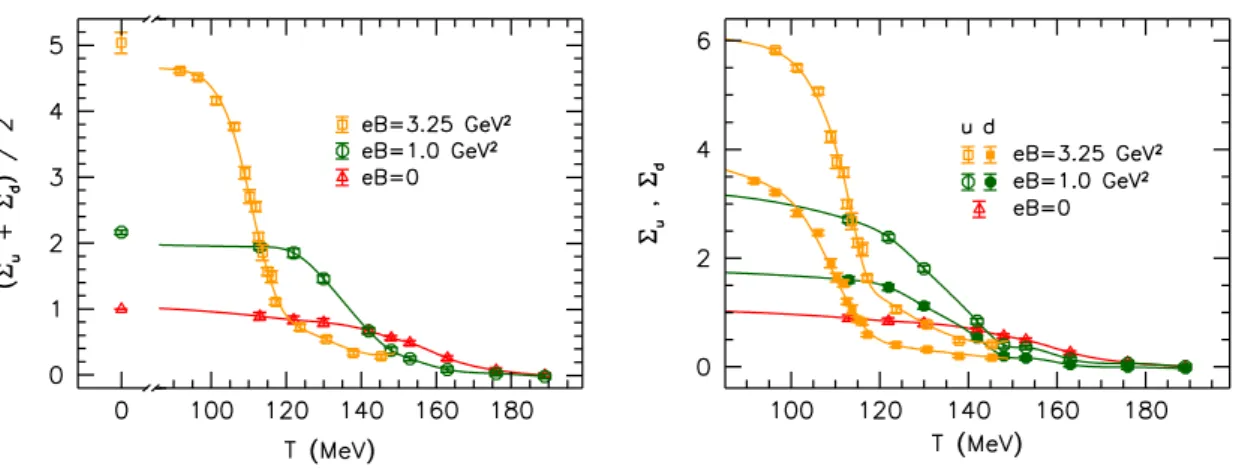
Let us start the discussion with the light quark condensates. The average of Σu and Σ_d is plotted in the left panel of figure 1, compared to the B = 0 and B = 1 GeV² continuum extrapolated results [7]. In addition to the data at nonzero temperatures, we also indicate an estimate for the zero-temperature condensate. This is obtained by fitting and extrapolating the available lattice data at T = 0 by a free-theory inspired form

∼BlogB. The systematic uncertainty is taken into account by varying the fit interval.

JHEP07(2015)173

Figure 1. Left panel: average light quark condensate as a function of the temperature for three different magnetic fields. Right panel: up (open points) and down (filled points) quark condensates for the same set of magnetic fields. The curves are spline interpolations and merely serve to guide the eye.

While the condensate is increased by the magnetic field at low temperatures, reflecting the well-known magnetic catalysis effect, the results also clearly show the reduction of Σ_u+ Σ_d in the transition region. Thus, inverse magnetic catalysis is observed to persist in the transition region even for our strong magnetic field eB = 3.25 GeV², pushing Tc

further down. In particular, we employ the inflection point of the average condensate to find T_c{Σ_ud} = 112(3) MeV. As a side-remark, we mention that since the transition region is shifted to considerably lower temperatures, the vacuum values determined for 3.45 < β < 3.85 in refs. [6, 7] suffice to perform the additive renormalization of the condensates, and there is no need for additional T = 0 simulations on finer lattices.

Due to the different electric charges, Σuis expected to be more sensitive to the magnetic field than Σ_d. On that account, even a splitting in the transition temperatures might seem plausible, see refs. [39,42]. To check whether this is the case, in the right panel of figure1the two condensates are plotted separately. Even though the difference Σu−Σ_dis pronounced throughout the temperature range in question, fitting for the inflection points gives consistent values Tc{Σ_u} = 112(3) MeV and Tc{Σ_d} = 111(3) MeV. An apparent implication of this finding is that the temperature, at which the transition between the chirally broken and restored phases takes place, is encoded in the gluonic configurations rather than in the operator insertion. In lattice language; Tc seems to be a quantity driven predominantly by sea and not by valence effects. This also suggests that purely gluonic observables would also exhibit similar transition temperatures.

This brings us to the simplest, purely gluonic quantity: the Polyakov loop (2.5). The (real part of the) renormalized observable is plotted in the left panel of figure 2, for the same set of magnetic fields, and is observed to be drastically enhanced by the magnetic field for all temperatures. The inflection point of Pr(T) is much more pronounced as compared to the case at B = 1 GeV² and is determined to be Tc{P} = 109(3) MeV.

This value is indeed consistent with the transition temperatures obtained above for the

JHEP07(2015)173

Figure 2. Left panel: the Polyakov loop for three values of eB. At the highest magnetic field, the curve is a spline interpolation, while for the lower fields the band is the result of a combined continuum extrapolation and interpolation in T [8]. Right panel: the strange quark number susceptibility for the same set of magnetic fields. For the highest magnetic field, a spline interpolation is shown, whereas for the lower fields the bands represent a continuum estimate based on the results of ref. [6].

light quark condensates. We conclude that the gluonic configurations are vastly different on the two ‘sides’ of the transition, and predestine the behavior of the light condensates, independently of the electric charge that appears in the operator. We also observe the strange quark number susceptibility to exhibit an analogous trend, see the right panel of figure 2. Performing a similar fit as for P_r, we obtain T_c{c^s₂}= 109(3) MeV.

A further observable of interest for the QCD equation of state is the trace anomaly (2.10). It measures the breaking of conformal symmetry by the glu- onic condensate, by the quark condensates and by the magnetic field itself. As B grows, the latter effect becomes dominant and I^(Φ) is increased drastically,

Figure 3. The trace anomaly for three different magnetic fields. Note the logarithmic scale.

as visible in figure 3. Since I^(Φ) contains B-dependent con- tributions already at zero tem- perature, the usual normalization I^(Φ)/T⁴ is not useful [13]. This large T = 0 contribution also damps the behavior of I^(Φ) in the transition region. The small kink aroundT_c, moving towards smaller temperatures as B grows, is to some extent still visible. We note that in order to determine fur- ther quantities related to the equa- tion of state (e.g. pressure, entropy density etc.), one would need ad-

JHEP07(2015)173

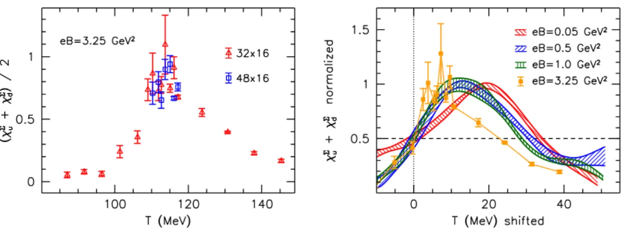
Figure 4. Left panel: finite size scaling of the average light quark susceptibility. Right panel: the dependence of the peak width on the magnetic field.

ditional simulations at low temperature (see the method developed in ref. [13]). This is outside the scope of the present paper.

Besides the characteristic temperature, the strength of the transition at high magnetic fields is also of interest. To determine, whether the smooth crossover ateB <1 GeV²turns into a real phase transition at eB= 3.25 GeV², we analyze the average of the light quark susceptibilitiesχ^Σ_u+χ^Σ_d. This observable exhibits a peak at the transition temperature, see the left panel of figure4. For real phase transitions, the heighthof this peak diverges in the infinite volume limit: h∝V for first-order transitions andh∝V^α with a critical exponent α <1 for second-order transitions. In contrast, for the case of an analytic crossover, h is independent of the volume. To perform this finite size scaling study, we compare the results obtained on the 48³×16 and on the 32³×16 ensembles. The left panel of figure 4shows no sign of a singularity asV is increased (note that for a first-order transition, the peak heights for the two volumes would differ by more than three). This leads us to conclude that the transition remains an analytic crossover even at eB = 3.25 GeV². We mention moreover that finite volume effects are also absent from the other observables discussed above.

Although the transition remains an analytic crossover, it is instructive to analyze the B-dependence of the susceptibility peak in more detail. We normalize χ^Σ_u +χ^Σ_d such that its peak maximum equals unity, and plot it in the right panel of figure 4 against the temperature. Here, T is shifted so that the observable equals 0.5 at zero. Then, the peak width w(B) at half maximum can be read off at the rightmost intersection of the observable with 0.5. Clearly, w(B) decreases as B grows, signaling that the transition becomes stronger in the presence of the magnetic field. We will return to this observation below in section5.

Besides being useful for quantifying the strength of the transition, the peak of the susceptibility allows for yet another determination of the transition temperature. Fitting for the peak maximum, we obtain Tc{χ^Σ_ud} = 113(4) MeV, consistent with the results obtained for all other observables. We mention that the peak positions for the up and down quark susceptibilities also agree within errors.

JHEP07(2015)173

Figure 5. The QCD phase diagram in the magnetic field-temperature plane. Previous results at weaker magnetic fields [6] are complemented by our findings at high eB. The points have been slightly shifted horizontally for better visibility. The dotted and the dashed lines show an interpolation of the results for Σu+ Σd and forc^s₂, respectively, according to eq. (3.1).

T_c(0) a₁ a₂ Σ_ud 160(2) MeV 0.54(2) 0.82(2)

c^s₂ 174(2) MeV 0.78(1) 1.28(1) Table 1. Fit parameters of the function (3.1).

Finally, in figure5we summarize our determinations ofT_c in the QCD phase diagram.

We consider the results for eB < 1 GeV² obtained for the light quark condensates and for the strange quark number susceptibility [6]. In addition, we also include the transition temperatures at eB = 3.25 GeV² obtained using the light quark condensates, the strange quark number susceptibility and the Polyakov loop. (Note that the inflection point of Prat eB <1 GeV² is not pronounced enough to allow for a stable fit.) To interpolate T_c{Σ_ud} and Tc{c^s₂} for all magnetic fields, we found the following function sufficient,

T_c(eB) =T_c(0)·1 +a₁(eB)²

1 +a2(eB)², (3.1)

giving the fit parameters shown in table 1. The resulting fit is also shown in the figure.

4 Results in the asymptotic magnetic field limit

Our results in the right panel of figure4 indicate that the transition becomes significantly sharper as the magnetic field increases. This observation raises the question: what happens if B is even larger? Does the crossover terminate and turn into a real phase transition?

To answer this question, we have to consider the limit eB Λ²_QCD. Asymptotic freedom dictates that in this limit quarks and gluons decouple from each other. Still, the explicit breaking of rotational symmetry by B and the corresponding dimensional reduction in the quark sector [10] suggests that this limit is not simply given by a pure gluonic theory

JHEP07(2015)173

plus non-interacting (electrically charged) quarks. Indeed, based on the structure of the gluon propagator in strong magnetic fields, ref. [43,44] has shown that the effective action describing this limit is an anisotropic pure gauge theory. The anisotropy amounts to an enhancement of the chromo-dielectric constant in the direction parallel to the magnetic field, characterized by the coefficient κ,

eB Λ²_QCD : L= 1 g²

h

trB_k²+ trB_⊥² + (1 +g²κ(B)) trE_k²+ trE_⊥²i

, κ(B)∝B.

(4.1) The definition of the gluonic field strength componentsBandEis given in eq. (A.2) below.

The enhancement of the parallel chromo-dielectric constant implies that the corresponding field strength componentE_kis suppressed. This tendency is already visible in our full QCD simulations at strong magnetic fields, see figure 11in appendix A below.

Therefore, asB is increased, the QCD effective Lagrangian approaches the anisotropic gauge theory given by eq. (4.1). Assuming that this theory has a first-order phase tran- sition, ref. [35] has conjectured that the strong magnetic field region of the QCD phase diagram should exhibit a critical point. Here we address this question in more detail.

First of all, in appendix A, we reproduce the results of ref. [43,44] for the magnetic field- induced anisotropy using the effective action in the Schwinger proper-time formulation.

The resulting anisotropic gauge theory can be simulated directly on the lattice. The setup and the simulation algorithm are described in appendix B. The main difference to simple pure gauge theory amounts to multiplying the plaquettes lying in the z−t plane by the anisotropy coefficient κ. The exact form of the anisotropic action is given in eq. (B.2).

Before discussing the lattice simulations of the anisotropic theory, let us make one more remark. Besides writing down the effective Lagrangian (4.1), ref. [43, 44] also predicted that the scaleλQCDof this theory (generated through dimensional transmutation) is much smaller than the QCD scale at B = 0: λ_QCD Λ_QCD for a very broad range of magnetic fields. In the absence of further dimensionful scales in the anisotropic theory, this implies that the deconfinement transition temperature for strong mangetic fields is also much smaller than T_c(B = 0). Below we will also address this prediction.

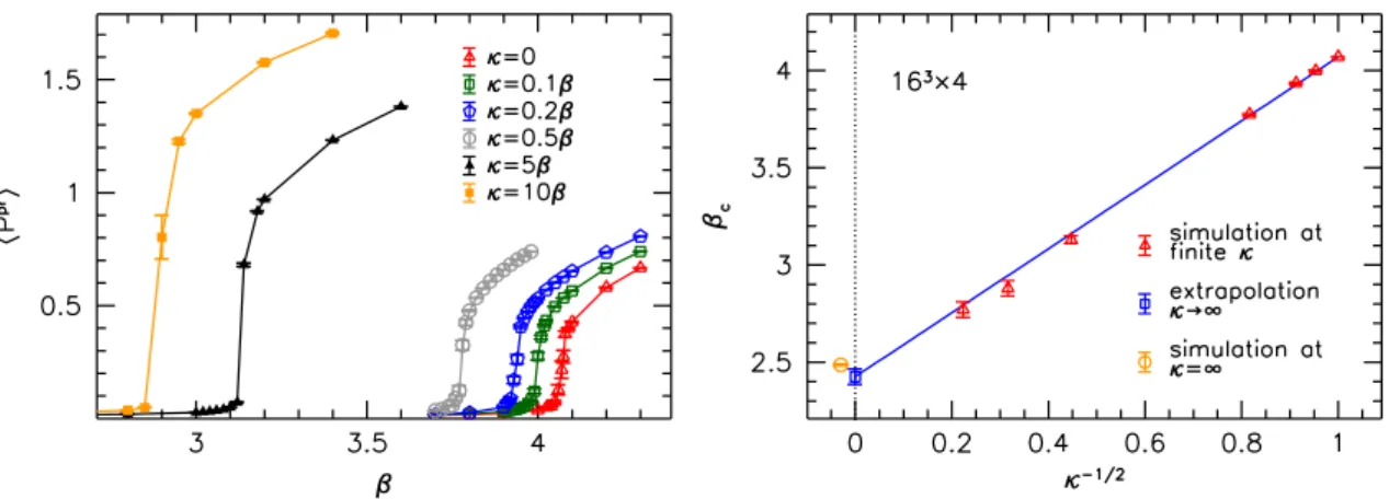
Due to the exact Z(3) symmetry of the anisotropic theory, the deconfinement transi- tion is characterized by the projected Polyakov loop (2.6). In the left panel of figure 6, this observable is plotted against the inverse gauge coupling β for several values of κ, as measured on the 16³×4 lattices. At κ = 0, we reproduce the results of refs. [49, 50] — in particular, the deconfinement transition occurs at βc ≈ 4.07. The results indicate βc

to be strongly reduced as κ grows.¹ We find that β_c scales approximately with 1/√ κ, see the right panel of figure 6. Extrapolating to κ = ∞ we obtain βc(κ = ∞) ≈ 2.42(5).

Besides approaching this limit via finite values of the anisotropy coefficient, we also de- velop an algorithm to simulate directly atκ=∞. The corresponding setup is described in appendix B.

The left panel of figure 7 shows P^pr at infinite anisotropy. We find that the critical inverse coupling on the 16³ ×4 lattice is comparable with the extrapolation based on

1Here we simulated at fixed values of the ratioκ/β. This continuous rescaling ofκhas no effect on, for example, the critical inverse coupling.

JHEP07(2015)173

Figure 6. Left panel: the projected Polyakov loop as a function of the inverse gauge coupling for various values of the anisotropy coefficient, as measured on the 16³×4 lattices. The solid lines merely serve to guide the eye. Right panel: the critical inverse coupling as a function of 1/√

κ. The extrapolation toκ=∞is compared to the result of the direct simulation at infinite anisotropy (the latter shifted horizontally for better visibility).

Figure 7. The projected Polyakov loop as a function of the inverse gauge coupling atκ=∞, for various lattice volumes withNt = 4 (left panel) andNt= 8 (right panel). The solid lines merely serve to guide the eye.

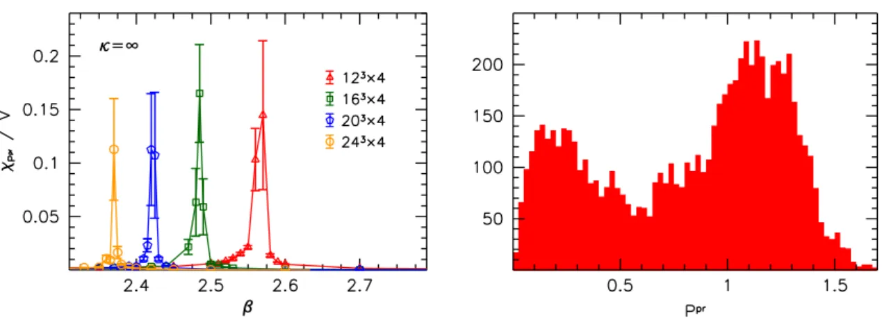
finite anisotropies, see the right panel of figure 6. In addition, a comparison of the results at different spatial volumes 12³. . .24³ reveals that the transition becomes sharper as the volume increases, as typical for real phase transitions. We also repeated this analysis on Nt= 8 lattices, see the right panel of figure 7. The critical couplings are clearly different, showing that the transition is indeed related to the finite temperature. We also mention that finite volume effects inβcare observed to be unusually large — above 10% for Nt= 4.

(For comparison, the finite volume effects atκ= 0 on similar lattices are of 0.1% [49].) We suspect that this is due to lattice artefacts — indeed, the effect is considerably smaller for Nt= 8, see the right panel of figure7.

To determine the nature of the transition, we calculated the susceptibility of the pro-

JHEP07(2015)173

Figure 8. Left panel: the susceptibility of the projected Polyakov loop, normalized by the spatial volume, as a function of the inverse coupling. Various spatial volumes with N_t= 4 are compared.

The solid lines serve to guide the eye. Right panel: histogram of P^pr near the critical temperature on the 16³×4 lattices.

jected Polyakov loop (2.7). This observable is shown in the left panel of figure 8, with a normalization by the spatial volume. Within statistical errors, the height of the normalized susceptibility peak is observed to be independent of V. In other words, the peak height scales linearly withV, which we take as strong evidence that the transition is offirst order.

The histogram ofP^pratβ= 2.4855 as measured on the 16³×4 lattices is shown in the right panel of figure8, revealing the two-peak structure characteristic for first-order transitions.

Through the equivalence between this anisotropic gauge theory and QCD with asymp- totically strong magnetic fields, the above finding implies that the QCD phase diagram exhibits a critical point in the strong magnetic field region, where the crossover turns into a real phase transition. Based on our full QCD results for the light quark susceptibilities, we will estimate the magnetic field corresponding to the critical point in section 5.

The next step is to relate the critical inverse couplingβc to the critical temperatureTc

in physical units. To do so, we must set the lattice scale β(a). In principle, the magnetic field is not expected to change this scaling relation (cf. ref. [6]). However, to arrive at our anisotropic gauge theory, B has been taken to infinity, i.e. it also exceeds the squared lattice cutoff a⁻². Clearly, the lattice scale determined at B = 0 becomes invalid beyond this point. Thus, in order to determine the lattice spacing, one needs a dimensionful quantity whose value is known in the asymptotic limit — for example a purely gluonic observable, where theB-dependence is expected to be only mild. A possible candidate for this role is the parameter w0 defined from the gradient flow of the gauge links [51] that is often used for scale setting in QCD, as suggested in ref. [52].

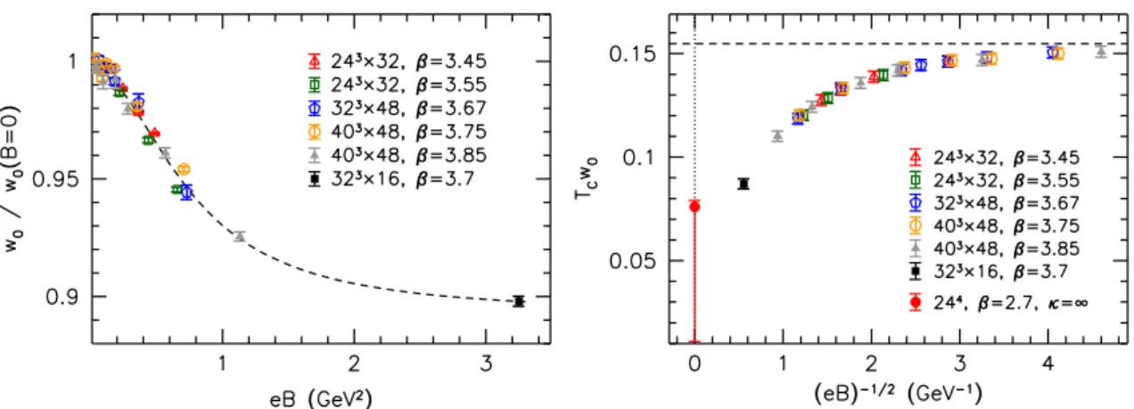
We determined w0 on our zero-temperature full QCD ensembles [7] foreB <1 GeV² and also foreB = 3.25 GeV² at our lowest temperature T ≈75 MeV. The results for the ratio w0/w0(B = 0) are plotted in the left panel of figure 9, showing a mild reduction of this parameter asB grows. A fit of the form similar to eq. (3.1) describes the data well and suggests a saturation towards the asymptotically strong magnetic field limit. Nevertheless,

JHEP07(2015)173

Figure 9. Left panel: magnetic field-dependence of the parameterw₀using various lattice spacings and a fit (dashed line) of the form similar to eq. (3.1). Right panel: the dimensionless combination Tcw0 in full QCD (1/√

eB >0.5 GeV⁻¹) and in the anisotropic pure gauge theory (1/√

eB = 0).

The dashed line indicates theB= 0 limit.

we cannot exclude a significant dependence of w₀ on B forB >3.25 GeV².

In addition, we can also gain some insight by considering the dimensionless combination T_cw₀. How close full QCD at eB = 3.25 GeV² is to the asymptotic limit can then be quantified by matchingTcw0with the anisotropic theory. Multiplying our full QCD results for w0 by the transition temperature (here we take the definition of Tc employing the inflection point of the strange quark number susceptibility, cf. figure 5), T_cw₀ is shown in the right panel of figure 9. Motivated by the scaling of βc (cf. the right panel of figure 6), the results are plotted against 1/√

eB. Employing the result for w₀ from ref. [52], at zero magnetic field we haveT_c(B = 0)·w₀(B = 0) = 0.174(3) GeV·0.1755(19) fm = 0.155(3).

To carry out the comparison to the asymptotic limit, we also determinedw0/aon sym- metric 16⁴and 24⁴ anisotropic gauge configurations at the critical couplings corresponding to the 16³×4 (βc ≈ 2.47) and to the 24³ ×8 (βc ≈ 2.7) lattices.² We observe that the combination Tcw0 = w0(βc)/a·1/Nt — similarly to βc — suffers from large lattice dis- cretization effects and exhibits a downwards trend towards the continuum limit. We take the result for theNt= 8 data as an upper limit, giving limB→∞(Tcw0).0.076. This value is also included in the right panel of figure 9. Altogether, the results are compatible with a monotonous dependence of T_cw₀ on B. To extrapolate T_cw₀ reliably to the continuum limit in the anisotropic theory requires further simulations on finer lattices and will be discussed in a forthcoming publication.

To summarize, the lattice results favor a saturation of w0 and a monotonous reduction of Tcw0 as the limit B → ∞ is approached. This suggests a monotonous reduction of T_c(B) towards the asymptotic limit. Nevertheless, based on the available findings, no final statement about limB→∞Tc can be made.

Let us make one more remark about the κ=∞ anisotropic theory. Since the parallel chromoelectric component trE_k²of the action vanishes, all plaquettes lying in thez−tplane

2Just as in full QCD, the gauge links are evolved here using the symmetric gradient flow.

JHEP07(2015)173

are unity. This implies that all Wilson loops W in this plane are trivial, and the static quark-antiquark potential∝logW is independent of the distance. Accordingly, there is no force acting on quark-antiquark pairs if they are separated in the direction of the magnetic field, i.e. the string tensionσ_k in this direction vanishes. This is in line with recent lattice determinations of the string tension in magnetic fields [53].

5 Conclusions

In this paper, we determined the nature and the characteristic temperature of the chi- ral/deconfinement transition of QCD at an extremely strong background magnetic field eB= 3.25 GeV². The results for various observables consistently show that the transition temperature is further decreased compared to its value at lower magnetic fields. For the light quark condensates, the reduction ofTc is due to the so-called inverse magnetic catal- ysis: between eB = 1 GeV² and eB = 3.25 GeV², Σ_u and of Σ_d are significantly reduced in the transition region. At the same time, the condensates are enhanced by B both for T Tc and for T Tc (the latter effect is small, since the condensate is suppressed at high temperatures).

Comparing the behavior of the up and down quark condensates and that of the Polyakov loop also revealed that there is no splitting between the transition temperatures for the individual flavors, neither is there significant difference between the chiral and the deconfinement transition temperatures. On the contrary, the different definitions ofT_ctend to approach each other asB grows and ateB = 3.25 GeV² all observables exhibit a single transition temperature of around 109−112 MeV, see figure5. Furthermore, we performed a finite size scaling analysis of the light quark susceptibilities, which has revealed that there is no singularity in the infinite volume limit and, thus, the transition remains an analytic crossover even ateB= 3.25 GeV².

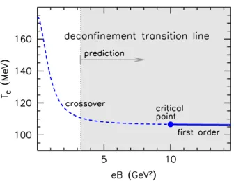
In addition, we considered the asymptotically strong magnetic field limit, and simu- lated the corresponding effective theory on the lattice. This limiting effective theory — an anisotropic pure gauge theory — was found to exhibit a first-order deconfinement phase transition. Together with our findings above, this implies the existence of a critical point in the QCD phase diagram. To provide a first estimate for the magnetic field BCP corre- sponding to the critical point, let us return to our results about the widthw(B) of the light quark susceptibilities. We have seen that the width is reduced as the magnetic field grows, see the right panel of figure 4. Assuming a linear dependence ofwon B and extrapolating in the magnetic field we find that w vanishes at

eBCP≈10(2) GeV². (5.1)

In light of the fact that the B-dependence of some of our observables (e.g. of Tc and of w₀) tends to flatten out as B grows, this first estimate should rather be taken as a lower bound for BCP. We mention that in order to simulate with magnetic fields of strengths comparable to that in eq. (5.1), lattices withNt&28 are required, out of reach for current computational resources.

JHEP07(2015)173

Figure 10. The deconfinement transition temperature against the background magnetic field. The results of our full lattice QCD simulations (white background) are complemented by the prediction (gray background) based on the results corresponding to theB → ∞limit and on the extrapolation of the light quark susceptibility peak to high magnetic fields (see the text).

In the absence of a priori known dimensionful scales in the B → ∞system, we could not determine limB→∞T_c in physical units. Nevertheless, the deconfinement transition temperature of the anisotropic theory is expected to be much smaller than T_c(B = 0) [43, 44].³ Our results for the combinationTcw0 are compatible with this prediction and suggest a gradual reduction of the deconfinement transition temperature asBis increased.⁴ Taking these aspects into account, figure 10 represents a sketch of the deconfinement transition line in the QCD phase diagram for a broad range of magnetic fields.

The reader might wonder whether it is possible that the crossover at eB ≤3.25 GeV² and the first-order transition in the asymptotic limit are not connected by a single line.

To see that this is not the case, note that by varying the anisotropy parameter κ, one can continuously deform the anisotropic theory to usual pure gauge theory, as was demonstrated in figure 6. Furthermore, the isotropic pure gauge theory can be thought of as QCD with infinitely heavy quarks and thus can be continuously transformed into full QCD by increasing the inverse quark masses from zero to their physical values. Thus, the transition we identified at B → ∞ is indeed the same deconfinement transition that occurs at low magnetic fields.

3The discussion in ref. [43, 44] bases on renormalization group arguments and on the separation of scales λQCD md √

eB (here λQCD is the dynamical scale of the large-B theory) to conclude that λQCD ΛQCD for a very broad range of magnetic fields — in fact, up to eB being millions of orders of magnitudes larger than Λ²_QCD. To find the completeB-dependence of the running of the strong coupling and to prove rigorously thatλQCD ΛQCD even in the B → ∞ limit, a full treatment of the divergent one-loop Feynman diagrams in the presence of background magnetic fields would be necessary. Without relying on the lowest-Landau-level approximation — which might not be justified for the case of divergent diagrams — this is a very difficult task.

4Note that our setup atB → ∞describes the low-energy effective action for gluons. Thus, the results in the anisotropic theory have no implications for the chiral transition. For more details on this point, see ref. [43,44].

JHEP07(2015)173

Let us highlight that according to this discussion, having a decreasing deconfinement transition temperature is actually natural to QCD. Furthermore, since theB → ∞limit is independent of the quark masses,⁵ a similar reduction of T_c by the magnetic field should also take place in QCD with heavier-than-physical quarks. However, in the latter case this reduction most probably follows an initial increase in the transition temperature, cf.

refs. [6, 54]. Indeed, recent lattice results employing overlap fermions and pion masses of about 500 MeV indicate inverse catalysis to occur around the transition temperature at the magnetic field eB≈1.3 GeV² [9].

Finally, we note that magnetic fields well above the strength (5.1) are predicted to be generated during the electroweak phase transition in the early universe [55]. If these fields remain strong enough until the QCD epoch, the emerging first-order phase transi- tion might have several exciting consequences. Via supercooling, bubbles of the confined phase can be formed as the temperature drops belowTc, leading to large inhomogeneities, important for nucleosynthesis [56]. Collisions between the bubbles can also lead to the emission of gravitational waves and, thus, leave an imprint on the primordial gravitational spectrum [57]. An absence of such signals, in turn, would imply an upper limit for the strength of the primordial magnetic fields.

Acknowledgments

This work was supported by the DFG (SFB/TRR 55). The author thanks Igor Shovkovy for valuable comments and Gunnar Bali, Bastian Brandt, Falk Bruckmann, Jan Pawlowski, K´alm´an Szab´o and Andreas Sch¨afer for enlightening discussions.

A Effective action in the asymptotic magnetic field limit

In this appendix we demonstrate how asymptotically strong magnetic fields induce an anisotropy in the gluonic sector using an Euler-Heisenberg-type approach. The QCD ef- fective Lagrangian in Euclidean space-time is

L(B) = 1

2g²trG_µνG_µν+L^q(B, G_µν), L^q(B, G_µν) =− X

f=u,d,s

log det

D(q/ _fB, G_µν)+m_f , (A.1) and the quark determinant will be regularized using Schwinger’s proper time formula- tion [58]. Since the electromagnetic field exceeds all scales in the system and in particular, (eB)² trG²_µν, we may approximate the the chromo-fields in the fermionic action to be weak. In addition, we assume the chromo-fields to be covariantly constant, D_µG_νρ= 0 to enable a fully analytical treatment of the problem. Given this condition, the field strength can be gauge transformed to be constant in space-time and diagonal in color space [59], G_µν = diag(G_µνc) with the color index c= 1,2,3.

5As long as the quark masses are finite — note that the m → ∞ and B → ∞ limits cannot be interchanged.

JHEP07(2015)173

Let us decompose the chromo-fields to chromomagnetic/chromoelectric components, B_k =G_xy, B_⊥= Gxz+Gyz

2 , E_k =G_zt, E_⊥ = Gxt+Gyt

2 , (A.2)

parallel or perpendicular to the electromagnetic field B. The leading terms in the strong B-expansion are quadratic in the chromo-fields and thus, to find the coefficients of the respective components, it suffices to consider separately the effect ofB andB_k,BandB_⊥,B andE_k andBandE_⊥. The effective Lagrangian for these components for small background magnetic fields was determined in refs. [48,60]. A similar calculation, generalized to finite temperatures and constant Polyakov loop backgrounds was performed in refs. [8,61].

Let us first take the case of B and B_k. For each flavor we may choose our coordinate system such thatq_fB is positive. Then, each color component experiences a total (positive) magnetic fieldq_fB+B_kc so that

L^q(B,B_k) = 1 8π²

X

f,c

m²_f(qfB+B_kc) Z ds

s² e^−s coth(q_fB+B_kc)s

m²_f . (A.3) SinceB_kc only appears in the sum withq_fB, the effective Lagrangian becomes independent of the chromomagnetic field in the limit qfB B_kc. This implies that quarks become insensitive toB_k, i.e. decouple from this gluonic component.

Next we take the case with B and B_⊥. Rotating our coordinate axes for each color component such that thez axis points in the direction of the total magnetic field we get

L^q(B,B_⊥) = 1 8π²

X

f,c

m²_f q

(q_fB)²+B²_⊥c Z ds

s² e^−s coth q

(qfB)²+B²_⊥cs

m²_f . (A.4)

In the strong B limit, this becomes independent of B_⊥c, signaling that quarks decouple from the perpendicular chromomagnetic component of the gluons as well.

For a perpendicular chromoelectric field, for each color component we can perform the Lorentz transformation that eliminates the electric field and, in turn, gives a total magnetic field

q

(q_fB)²+E_⊥c² . The corresponding effective Lagrangian equals eq. (A.4), but withB_⊥creplaced byE_⊥c. This implies the decoupling of quarks from the perpendicular chromoelectric fields.

Finally, for a parallel chromoelectric field E_k, we have a Landau problem in the x−y as well as in the z−tplanes, giving

L^q(B,E_k) = 1 8π²

X

f,c

q_fBE_kc Z ds

s e^−s cothqfBs

m²_f cothE_kcs

m²_f . (A.5) Taking the limit q_fB E_kc, m²_f, we see that — unlike for the other components above

— a non-trivial dependence on E_k remains. We are interested in the quadratic term,

JHEP07(2015)173

proportional to trE_k², which contributes⁶ to the gluonic Lagrangian trG²_µν of eq. (A.1), L^q(B,O(E_k²)) = 1

24π² X

f,c

qfB E_kc² m²_f

Z

ds e^−s =κ(B) trE_k², κ(B)≡ 1 24π²

X

f

|q_f/e||eB|

m²_f . (A.6) Altogether, the asymptotically strong magnetic field limit of the QCD effective Lagrangian indeed equals eq. (4.1). Thus we find that the chromo-dielectric constant is enhanced in the direction of the background magnetic field, and the coefficientκ(B) coincides with the result of ref. [43,44].

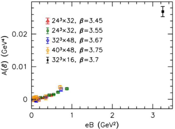
Figure 11. The anisotropy of the chromoelectric gluonic field strength component in full QCD.

Having κ 1 in the ac- tion implies that the correspond- ing gluonic field strength compo- nent trE_k² is strongly suppressed.

In other words, the anisotropy in the chromoelectric part of the ac- tion density,

A(E) = 1 V₄

1 g²

D

trE_⊥² −trE_k²E , (A.7) is enhanced by B. To back up this prediction, in figure 11 we plot A(E) as a function of the magnetic field, based on our zero-

temperature results at eB < 1 GeV² [48] and the measurements at eB = 3.25 GeV² at our lowest temperature T ≈ 75 MeV. The results clearly indicate that the anisotropy is positive and strongly increased as B grows. We note that due to the coupling between the gluonic field strength components, a similar anisotropy in the chromomagnetic sector also appears, altogether giving rise to the hierarchy trB_k² > trB²_⊥ = trE_⊥² > trE_k² at low temperatures. The same hierarchy is also observed in the anisotropic gauge theory.⁷

We note that the calculation leading to eq. (4.1) can also be performed for nonzero temperatures. AtT >0 an additional factor appears in the proper time integral due to the sum over Matsubara frequencies, containing an elliptic Θ-function. This factor decouples

6Here we omitted a divergent term of the form trEk²log Λ/mf, where Λ is a cutoff entering as the lower endpoint of the proper time integrations0∝1/Λ². This divergence can be eliminated by the multiplicative renormalization of the wave functionEkand of the gauge coupling g[58]. Closer inspection of eqs. (A.3) and (A.4) shows that the same type of divergence is present for the other components as well. Thus, these B-independent terms merely represent an isotropic redefinition of the gauge coupling g, which does not alter the form of the effective Lagrangian for strong magnetic fields. Another divergence, independent of the gluonic field strengths, takes the form (qfB)²log Λ/mf and is canceled by the renormalization ofBand ofqf [58]. Thus, the necessary renormalizations atB→ ∞are of the same type as for the theory at small magnetic fields.

7To see how the anisotropic dielectricconstant affects the chromomagneticcomponents, it is instructive to consider the gauge potentialAµ. A large value ofκimplies a suppression of trE_k² and a corresponding suppression of the fluctuations inAz and inAt. This suppression propagates into the magnetic sector and creates the anisotropy between trB⊥² and trBk². Indeed, while the former containsAz, the latter does not.

JHEP07(2015)173

from theB-dependence, implying that even forT >0, only the chromo-dielectric constant is affected. The coefficientκ is, however, altered as

κ(B, T) = 1 24π²

X

f

|q_f/e||eB|

m²_f Z

ds e^−sΘ3

hπ

2, e^{−m2f/(4sT2)} i

. (A.8)

The integral over s equals unity at T = 0 and is reduced monotonously (and smoothly) as the temperature grows. Simulating the anisotropic gauge theory according to the La- grangian (4.1) on the lattice, we found that the theory exhibits a first-order phase transition.

Thus, since the smooth κ(T) dependence does not affect the discontinuous transition, in order to locate the critical temperature it suffices to simulate the theory at fixed (large) κ values.

B Simulating anisotropic pure gauge theory on the lattice

In this appendix we discuss the simulation algorithm for the anisotropic pure gauge theory described by the Lagrangian (4.1). The corresponding path integral

Z = Z

DU e^−βSanisog , (B.1)

can be simulated directly on the lattice. Here, U denotes the gauge links, β = 6/g² is the inverse gauge coupling and the anisotropic gauge action reads

S_g^aniso =X

µ<ν

1

3Re trPµν·κµν, κµν =

(1 +κ(B)/β, µ=z, ν=t,

1, otherwise, (B.2)

wherePµνare linear combinations of closed loops lying in theµ−ν plane. We take the tree- level Symanzik improved gauge action such that these loops include the 1×1 plaquettes U_µν^1×1 and the 2×1 rectanglesU_µν^2×1 with appropriately tuned coefficients [62],

Pµν =− 1

12 1−U_µν^2×1 +5

3 1−U_µν^1×1

. (B.3)

The correspondence between the continuum and lattice expressions reads

trE_k²= 2RetrPtz, trE_⊥² = Retr [Ptx+Pty], trB_k² = 2RetrPxy, trB²_⊥= Retr [Pyz+Pxz].

(B.4) To simulate this theory, we use an overrelaxation/heatbath algorithm, based on the isotropic pure gauge implementation by the MILC collaboration [63]. One trajectory con- sists of one overrelaxation step followed by four heatbath steps. The simulation at finite anisotropy coefficient κ simply involves multiplying the plaquettes and rectangles lying in the z−t plane by κ. We observe that autocorrelation times grow large as κ increases, similarly to the issue of critical slowing down of the isotropic theory at large β. This pro- hibits approaching κ → ∞, necessary for the asymptotically strong magnetic field limit.

However, it is possible to modify the algorithm to simulate directly at κ = ∞. In this limit, the z−tcomponent of the action and the remaining five components decouple, and

JHEP07(2015)173

the links are restricted to the subspace Ω[U] of configurations, whereP_zt is minimal. This subspace is defined by

Ω[U] ={U_µ|U_zt^1×1 =1}. (B.5)

Indeed, any fluctuation in the link variables that leads off of this subspace makes the action infinitely large and is thus forbidden. (Note that if U_zt^1×1 equals the unit matrix, then so does U_zt^2×1.)

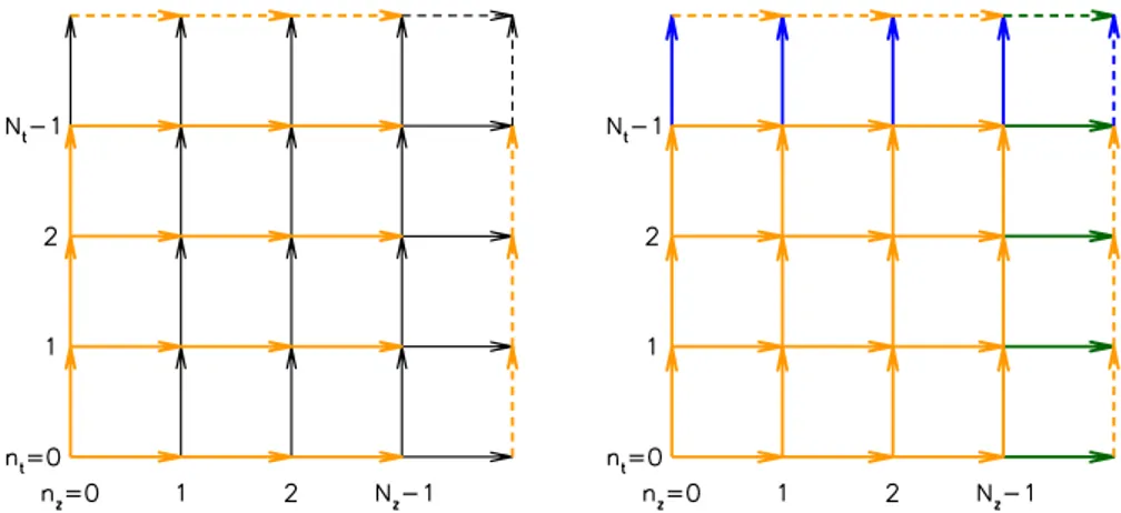
We thus have to parameterize the subspace Ω[U] in terms of the gauge links Uµ. Let us label the lattice sites by n= (nx, ny, nz, nt) with 0 ≤ nµ < Nµ. To find the parame- terization of eq. (B.5), it is advantageous to fix the links to 1on a so-called maximal tree.

The specific choice for the tree is shown in the left panel of figure 12. (Note that Faddeev- Popov fields are absent for such a gauge fixing [64].) In order to have unit plaquettes for n_z < N_z −1 and n_t < N_t−1, all t-links must be set to unity at these sites. To have unit plaquettes on the last z-slice, allz-links atNz−1 must be set equal, denoted by Lz. Similarly, all thet-links atN_t−1 must be set equal, denoted byL_t, see the visualization in the right panel of figure12. These remaining links correspond to the local Polyakov loops in the z- and in the t-direction, lying in the z−t plane at a given nx and ny. Finally, to ensure that the plaquette at the corner n_z = N_z −1, n_t = N_t−1 is unity, we need LzLtL^†zL^†_t =1, i.e. Lz andLt must commute. Altogether, the subspace in question reads

Ω[U] ={U_µ|U_z(n) =1∀n_z 6=N_z−1, U_t(n) =1∀n_t6=N_t−1,

Uz(nx, ny, Nz−1, nt) =Lz(nx, ny)∀n_t, Ut(nx, ny, nz, Nt−1) =Lt(nx, ny)∀n_z, [Lz(nx, ny), Lt(nx, ny)] = 0}.

(B.6)

Notice that the ‘degenerate’ timelike Polyakov loop L_t (represented by the blue arrows in the right panel of figure 12) appears multiple times in the action — in fact, in 4Nz

plaquettes and in 12N_z rectangles. The corresponding ‘staples’ are all taken into account in the update of L_t (and similarly forL_z).

There are several ways to fulfill the commutativity relation [Lz, Lt] = 0. One possibility (setup A) is to simply set L_z = 1 for all n_x and n_y. Another approach (setup B) is to constrainL_z to be a center element, L_z(n_x, n_y)∈Z3. The two setups only differ on a set whose measure vanishes in the limit, where all lattice extents are taken to infinity. Note that the expectation value of the average z-Polyakov loop P^(z) [defined similarly as the usual Polyakov loopP, eq. (2.5)] is three for setup A, whereas it is zero for setup B, if the spatial size of the system is large enough. Nevertheless, we checked that observables sensitive to the finite temperature transition (P, the gauge action, etc.) all have vanishing correlators withP^(z). In fact, we found that the setups A and B give identical results forP and for the gauge action for all values of the inverse gauge coupling β on the 16³×4 lattices. In other words, center symmetry breaking in thez direction appears to be completely irrelevant for the deconfinement phase transition.

In addition, we also tried allowing both Lz andLtto be general SU(3) matrices (which violates the commutativity relation). This approach (setup C) turned out to introduce