JHEP08(2014)177
Published for SISSA by Springer Received: June 10, 2014 Revised: August 5, 2014 Accepted: August 7, 2014 Published: August 29, 2014
The QCD equation of state in background magnetic fields
G.S. Bali,a,b F. Bruckmann,a G. Endr˝odi,a,1 S.D. Katzc,d and A. Sch¨afera
aInstitute for Theoretical Physics, Universit¨at Regensburg, Universit¨atsstraße 31, D-93040 Regensburg, Germany
bTata Institute of Fundamental Research, Homi Bhabha Road, Mumbai 400005, India
cE¨otv¨os University, Theoretical Physics,
P´azm´any P. s. 1/A, H-1117, Budapest, Hungary
dMTA-ELTE Lend¨ulet Lattice Gauge Theory Research Group, P´azm´any P. s. 1/A, H-1117, Budapest, Hungary
E-mail: gunnar.bali@physik.uni-r.de,falk.bruckmann@physik.uni-r.de, gergely.endrodi@physik.uni-r.de,katz@bodri.elte.hu,
andreas.schaefer@physik.uni-r.de
Abstract: We determine the equation of state of 2+1-flavor QCD with physical quark masses, in the presence of a constant (electro)magnetic background field on the lattice. To determine the free energy at nonzero magnetic fields we develop a new method, which is based on an integral over the quark masses up to asymptotically large values where the effect of the magnetic field can be neglected. The method is compared to other approaches in the literature and found to be advantageous for the determination of the equation of state up to large magnetic fields. Thermodynamic observables including the longitudinal and transverse pressure, magnetization, energy density, entropy density and interaction measure are presented for a wide range of temperatures and magnetic fields, and provided in ancillary files. The behavior of these observables confirms our previous result that the transition temperature is reduced by the magnetic field. We calculate the magnetic suscep- tibility and permeability, verifying that the thermal QCD medium is paramagnetic around and above the transition temperature, while we also find evidence for weak diamagnetism at low temperatures.
Keywords: Quark-Gluon Plasma, Lattice QCD, Phase Diagram of QCD ArXiv ePrint: 1406.0269
1Corresponding author.
JHEP08(2014)177
Contents
1 Introduction 1
2 Thermodynamics in an external magnetic field 3
3 Lattice observables and methods 5
3.1 Flux quantization and methods to determine the magnetization 6
3.2 Renormalization 7
3.2.1 Charge renormalization — free case 8
3.2.2 Charge renormalization — full QCD 9
3.3 The integral method at nonzero magnetic fields 10
3.4 Lattice ensembles 13
4 Results 13
4.1 Condensates, the β-function and a comment on magnetic catalysis 13
4.2 Quadratic contribution to the EoS 15
4.3 Complete magnetic field dependence of the EoS 18
4.4 Magnetic susceptibility and permeability 21
4.5 Entropy density and the Adler function 24
4.6 Phase diagram 26
5 Summary 27
A Expansion of the quark determinant 29
B Magnetic susceptibility in the HRG model 29
1 Introduction
Quantum Chromodynamics (QCD) is the theory of the strong interactions. Its most im- portant properties are the confinement of quarks and gluons at low energies and asymptotic freedom at high scales. Lattice simulations of QCD have unambiguously shown that at zero quark densities these two, fundamentally different regimes are connected by a smooth crossover-type transition [1, 2]. This transition — through which the dominant degrees of freedom change from composite objects (hadrons) to colored quarks and gluons — has several characteristics of both theoretical and phenomenological relevance. Besides the na- ture and the (pseudo)critical temperature of the transition, one such characteristic is the equation of state (EoS), which is the fundamental relation encoding the thermodynamic properties of the system.
JHEP08(2014)177
In particular, the EoS gives the equilibrium description of QCD matter, in terms of relations between thermodynamic observables like the pressure, the energy density or the entropy density. These observables enter hydrodynamic models that are used to describe the time evolution of the quark-gluon plasma (QGP) produced in heavy-ion collision exper- iments [3,4]. Besides its role in heavy-ion physics, the EoS affects the mass-radius relation of neutron stars [5] and enters cosmological models of the early universe, with implications, for example, for dark matter candidates [6].
Of particluar relevance is the response of the EoS to changes of the control parameters of the system. These parameters include the temperature, the chemical potentials conjugate to conserved charges and, in the present case, a background (electro)magnetic fieldB =|B|.
External magnetic fields play an important role in the evolution of the early universe [7], in strongly magnetized neutron stars [8] and in non-central heavy-ion collisions, see, e.g., the recent review [9]. Magnetic fields induce a variety of exciting effects in the thermodynamics of QCD — for example they significantly affect the phase diagram. The first results in this field were obtained using low-energy models and effective theories of QCD, see the summary in, e.g., ref. [10]. The QCD transition has also been studied extensively on the lattice; we refer the reader to reviews on the subject in, e.g., refs. [11–13]. A very relevant question in this respect has been the dependence of the transition temperatureTcand of the nature of the transition on the magnetic field. In this paper we also address this issue.
Our main objective is to determine the QCD EoS around the crossover transition at vanishing chemical potentials, for nonzero background magnetic fields. To this end we develop a generalization of the so-called integral method [14], which relies on an integration in the quark masses up to asymptotically large values (a similar integration in the quark masses atB = 0 was also considered in ref. [15]). We calculate thermodynamic observables including the pressure, the energy density, the entropy density, the interaction measure, the magnetization and the susceptibility for magnetic fields of up to eB = 0.7 GeV2 for a wide range of temperatures 110 MeV < T <300 MeV, allowing for a comparison with the Hadron Resonance Gas (HRG) model and with perturbation theory, at low and high temperatures, respectively. At highT we demonstrate that several aspects of perturbative QED physics are encoded in the EoS observables. Furthermore, our results confirm the observation made in refs. [16,17] that the transition region is shifted to lower temperatures as B grows. Another phenomenological consequence of the magnetic field is that the pressure — if defined as the response against a compression at fixed magnetic flux, see precise definition in section 2 below — becomes anisotropic, and a significant splitting between the components parallel and perpendicular toB is developed.
The change in the EoS due to the magnetic field has further theoretical implications.
QCD matter may be thought of as a medium with either para- or diamagnetic properties.
We establish that around and above the transition region the magnetization is positive and thus the thermal QCD medium behaves as a paramagnet, with a magnetic permeability larger than unity. A possible implication of this paramagnetism for heavy-ion collisions has been pointed out recently in ref. [18]. In addition, we present evidence for the emergence of a weakly diamagnetic region at low temperatures due to pions.
JHEP08(2014)177
This paper is organized as follows. First we discuss thermodynamic relations in the presence of the magnetic field from a general point of view in section 2. We proceed by describing the lattice methods that are used to determine the EoS in section 3, with spe- cial emphasis on the implications of flux quantization and electric charge renormalization.
Section4 contains our main results, followed by the conclusions in section5.
2 Thermodynamics in an external magnetic field
The fundamental quantity of thermodynamics is the free energy or thermodynamic poten- tial. In terms of the partition function Z of the system it reads F = −TlogZ. In the presence of an external magnetic field the density f =F/V of the free energy in a finite spatial volumeV can be written as [19]
f =−T s=total−T s−eB· M, (2.1)
where is the energy density of the medium, s the entropy density and Mthe magneti- zation. Without loss of generality, the magnetic field B =Bez is taken to point in the z direction, and for later convenience,Bis given in units of the elementary chargee >0. Note that the total energy of the system,total=+field, includes the energy of the mediumas well as the work necessary to maintain the constant external field,field =eB· M[20]. The two expressions in eq. (2.1) thus correspond to two different conventions for the definition of the energy density. The entropy density and the magnetization can be obtained as
1 V
∂F
∂T =−s, 1 V
∂F
∂(eB) =−M. (2.2)
The corresponding differential relation for the pressure is somewhat more involved.
Since the magnetic field marks a preferred direction, the pressures pi in the transverse (perpendicular to B) and in the longitudinal (parallel to B) directions may be different.
In ref. [21] we have shown that this possible anisotropy depends on the precise definition ofpi. Writing the volume as the product of linear extentsV =LxLyLz, the pressure com- ponents are related to the response of the system to compressions along the corresponding directions, i.e.
pi =−1 VLi
∂F
∂Li
. (2.3)
In order to unambiguously definepi, we have to specify the trajectory in parameter space, along which the partial derivative is evaluated. In ref. [21], we have distinguished between a setup where the magnetic fieldB is kept fixed during the compression (the “B-scheme”), and a setup where the magnetic flux Φ =eB·LxLy is kept fixed (the “Φ-scheme”). The B-scheme results inisotropic pressures, whereas the Φ-scheme givesanisotropic pressures:
p(B)x =p(B)y =pz, p(Φ)x =p(Φ)y =pz−eB· M. (2.4) The difference in the transverse components for the Φ-scheme is due to the fact that the compressing force in this case also acts against the magnetic field. Note that the definition of the pressures as spatial diagonal components of the energy-momentum tensor exhibits
JHEP08(2014)177
the Φ-scheme anisotropy [22]. This is due to the fact that the energy-momentum tensor is usually defined through the variation of the action with respect to the metric at fixed Φ, see ref. [21]. In contrast to px,y, the longitudinal pressure is independent of the scheme, and in the thermodynamic limit V → ∞ simplifies to
pz =−f. (2.5)
Note that the appropriate scheme to be used depends on the physical situation that one would like to describe. In particular, it is specified by the trajectoryB(Li), along which the compression perpendicular to the magnetic field proceeds. As will be explained below, in lattice regularization it is natural to keep the flux fixed, and thus, the lattice measurements correspond directly to the Φ-scheme. However, this does not represent a limitation of the lattice approach, since one can easily translate from one scheme into another. The pressure components for a general B(Li) trajectory (“general scheme”) can be found by combining our results for the longitudinal pressure and for the magnetization (both are contained in online resources on the paper’s page),
p(general)x =pz+M ·Lx∂(eB)
∂Lx . (2.6)
This relation reproduces the B- and Φ-schemes, eq. (2.4), for the trajectories B(Li) =B and eB(Li) = Φ/(LxLy), respectively.
Another important observable for the EoS is the interaction measure (trace anomaly),
I ≡−px−py −pz, (2.7)
which contains the energy of the medium and the three pressures. Thus, I also depends on the scheme:1
I(B)=−3pz, I(Φ)=−3pz+ 2eB· M, (2.8) whereas the energy density (likepz) is by construction scheme-independent,
=I(B)+ 3pz=I(Φ)+ 3pz−2eB· M. (2.9) Eqs. (2.1), (2.5) and (2.8) reveal that the entropy density can also be calculated as
s= +pz
T . (2.10)
Finally, the derivative of the magnetization with respect to B at vanishing magnetic field gives the magnetic susceptibility,
χB= ∂M
∂(eB) B=0
=−1 V
∂2F
∂(eB)2 B=0
. (2.11)
1One may understand the scheme-dependence ofIas follows. The trace anomaly represents the response to a rescaling of the length scaleξ in the system. To define this rescaling unambiguously, the trajectory B(ξ) has to be specified, i.e. a scheme has to be chosen. Hence,I becomes scheme-dependent. As a simple example, consider the magnetic field in the absence of particles. Taking into account the energyB2/2 of the magnetic field, one obtainsI(Φ) = 0, whileI(B) = 2B2. Notice that in the Φ-scheme a dimensionless number characterizes the magnetic field, whereas in theB-scheme we introduced a dimensionful parameter into the system. This is reflected by the vanishing of the trace anomaly in the former case, and the nonzero value ofI in the latter.
JHEP08(2014)177
3 Lattice observables and methods
In what follows we consider a spatially symmetric lattice with isotropic lattice spacing a.
Here the temperature and the three-volume are given by
T = (Nta)−1, V = (Nsa)3, (3.1)
whereNs andNt are the number of lattice sites along the spatial and temporal directions, respectively.
Using conventional Monte-Carlo methods the free energy F = −TlogZ itself is not accessible on the lattice, but only its derivatives with respect to the parameters of the theory. For the case of 2 + 1 flavor QCD coupled to a constant external magnetic field, these parameters are the inverse gauge coupling β = 6/g2, the lattice quark masses mfa (f =u, d, slabeling the flavors) and the magnetic flux Φ = (Nsa)2eB. In particular, in the staggered formulation of lattice QCD, Z is written as
Z= Z
DU e−βSg Y
f=u,d,s
detM(U, a2qfB, mfa)1/4
, (3.2)
where M = (D/ +mf)ais the fermion matrix, and the quark charges are set to qd =qs=
−qu/2 =−e/3. Note that the magnetic field has no dynamics, therefore the chargeqf (or, the elementary chargee) and the magnetic fieldBdo not appear separately in the partition function, but always in the combinationqfB (oreB). The constant Maxwell termB2/2 is independent of the physical properties of the thermal QCD medium and plays no role in the thermodynamics of the system. It only enters in the renormalization prescription, see section 3.2below.
We work with the tree-level improved Symanzik gauge action Sg, and stout improved staggered quarks in the fermionic sector. The detailed simulation setup is described in refs. [16, 23]. The quark masses are set to their physical values along the line of constant physics (LCP). This means that mfaare tuned as functions of β in a way that “physics remains the same”, that is to say, ratios of hadron masses measured on the lattice coincide with their experimental values. This defines the physical quark massesmphf afor each value of β. In particular, our LCP is set by fixing the ratio of the kaon decay constant to the pion mass fK/Mπ and the kaon decay constant to the kaon mass fK/MK. This results in the fixed ratio of quark masses mu =md≡mud =ms/28.15. The lattice spacing a(β) is set usingfK. For additional details on this procedure, see ref. [15].
The derivatives of logZ with respect toβ and mfaare the gauge action density and the quark condensate densities,
a4sg =− 1 Ns3Nt
∂logZ
∂β , a3ψ¯fψf = 1 Ns3Nt
∂logZ
∂(mfa). (3.3)
The interaction measure, eq. (2.7), can be given in terms of the response of the free energy to an overall change of length scales in the system. On the lattice this amounts to a derivative with respect to the lattice spacinga. Employing thea-dependence of the lattice
JHEP08(2014)177
parameters β and mfa, the densities of eq. (3.3) enter the Φ-scheme interaction measure in the following way:
I(Φ)=−T V
∂logZ
∂loga Φ
= ∂β
∂logasg−X
f
∂log(mphf a)
∂loga mfψ¯fψf. (3.4) Note that for the B-scheme interaction measure (see eq. (2.8)), an additional term con- taining the derivative with respect to the lattice fluxa2eB appears.
For convenience, we also define the change due to B for any observable X as
∆X ≡ X|B−X|0. (3.5)
The renormalization of the above observables will be discussed in section3.2.
3.1 Flux quantization and methods to determine the magnetization
Due to the periodic boundary conditions, the magnetic flux traversing the finite lattice is quantized as
Φ = (Nsa)2·eB= 6πNb, Nb ∈Z, 0≤Nb < Ns2, (3.6) where we took into account that the smallest charge in the system (that of the down quark) is qd = e/3. Note that since the flux is quantized, the lattice setup automatically corre- sponds to the Φ-scheme defined in section 2. Moreover, due to the quantization condition, differentiation with respect to eB is in principle ill-defined and therefore the magnetiza- tion of eq. (2.2) is not accessible directly. Recently, several methods were developed to circumvent this problem, which we summarize briefly below.
• Anisotropy method. One can make use of the relation (2.4) for the Φ-scheme, and express the magnetization as the difference between the longitudinal and transverse lattice pressures. These can be measured as derivatives of logZ with respect to anisotropy parameters. This approach was developed and successfully applied in refs. [18, 21]. The advantage of the method is that M is directly obtained as an expectation value for any B, while its drawback is that anisotropy renormalization coefficients also need to be determined.
• Half-half method. Instead of the uniform (and, thus, quantized) magnetic field, one can work with an inhomogeneous field which has zero flux, e.g. one that is positive in one half and negative in the other half of the lattice. Since the field strength is now a continuous variable, derivatives of logZ with respect toeBare well defined and can be measured on a B = 0 lattice ensemble [24]. The second-order derivative directly gives the magnetic susceptibility. However, higher-order terms become increasingly noisy, which limits the applicability of the approach to low fields. Note moreover that the discontinuities in the magnetic field may enhance finite volume effects.
• Finite difference method. The derivative of logZwith respect toeBis an unphys- ical quantity due to the quantization eq. (3.6). Still, this derivative can be measured
JHEP08(2014)177
for any real value of Nb, and its integral over Nb between two integer values gives the change in logZ between these two fluxes. In this way, logZ(Nb+ 1)−logZ(Nb) is constructed as the integral of an oscillatory function. The method is in principle applicable for any magnetic field, but 10-20 independent simulations are necessary to go from one integer flux to the next, making large magnetic fields computationally expensive [25,26].
• This work: generalized integral method.The method we will use in the present paper is based on two observations: that magnetic fields have no effect in pure gauge theory, and that the infinite quark mass limit of QCD (at a fixed magnetic fieldqB m2) is pure gauge theory. Based on this, the change in logZ due to the magnetic field can be expressed as an integral of the quark condensate differences ∆ ¯ψfψf over the quark masses, including unphysically heavy quarks. On a finite lattice, this integral is well regulated and can be calculated in a controlled manner by using 10-20 indepen- dent simulations for any given value of the magnetic field. Most of these simulations are at large quark masses, where the computation is significantly cheaper. Further- more, the method automatically gives information on the mass-dependence of logZ as well. This approach was sketched in ref. [27] and will be described in detail below.
3.2 Renormalization
The free energy density contains additive divergences in the cutoff — i.e. in the inverse lattice spacing. These divergences are independent of eB, except for one logarithmic di- vergence of the form −b1(eB)2log(µa), where µ is a renormalization scale. This term is canceled through a redefinition of the energy B2/2 of the magnetic field itself [28],
B2 2 = Br2
2 +b1(eB)2log(µa). (3.7)
Eq. (3.7) is equivalent to a simultaneous renormalization of the wave function (magnetic fieldB) and of the electric chargee. The combinationeBis renormalization group invariant and, as such, unaffected by this transformation:
Ze= 1 + 2b1e2rlog(µa), B2 =ZeBr2, e2 =Ze−1e2r, eB=erBr. (3.8) The purely magnetic contributionBr2/2 is trivial and can be omitted from the Lagrangian.
Therefore, the renormalization of the free energy amounts to adding the counter-term b1(eB)2log(µa) to ∆f. In the following it will be advantageous to consider the exten- sive quantity ∆ logZ = −L4∆f at zero temperature, in a box of four-volume L4. The counter-term then takes the form −b1Φ2log(µa) with the flux Φ =L2eB. The coefficient b1 of the divergence is related to the QED β-function [29–31]. Since the magnetic field is external, i.e. there are no U(1) degrees of freedom in the system, only the lowest order QEDβ-function coefficientb1 appears inZe(however, with a full dependence on the QCD coupling, see eq. (3.14) below).
JHEP08(2014)177
3.2.1 Charge renormalization — free case
It is instructive to first discuss the renormalization procedure in the free case — i.e. for elec- trically charged quarks in the absence of strong interactions. In this case the free energy can be calculated analytically (see, e.g., refs. [30–32]). We consider quark flavors of chargesqf and, for simplicity, we assume degenerate massesmf =mfor allf. The discussion is easily generalized to unequal masses. For Nc= 3 colors, the QEDβ-function coefficient reads
bfree1 =X
f
bfree1f , bfree1f = Nc
12π2 ·(qf/e)2. (3.9) At zero temperature, the expansion of ∆ logZ in the magnetic field is given by
∆ logZrfree=bfree1 ·Φ2·log(mfa) +O(Φ4)−bfree1 ·Φ2·log(µa), (3.10) where we also included the counter-term. Taking the derivative with respect to the mass of the quark flavorf, we obtain the corresponding quark condensate at T = 0,
∆ ¯ψfψffree= 1 L4
∂∆ logZrfree
∂mf =bfree1f (eB)2
mf +O((eB)4), (3.11) showing that the condensate contains no B-dependent divergences, and that it is also independent of the renormalization scale µ. Note also that the sign of the magnetic field- induced change in the condensate is, to leading order, determined by the sign ofbfree1f . Since QED is not asymptotically free, bfree1f is positive and the condensate undergoes magnetic catalysis at T = 0 to quadratic order in eB (we have already presented this argument in refs. [27, 32]). Note that approaching the chiral limit (i.e. eB/m2 → ∞), the magnetic field-expansion in eq. (3.11) becomes ill-defined. In fact, in the mf → 0 limit ∆ ¯ψfψffree vanishes (see, e.g., ref. [33]) for any magnetic field. However, the condensate difference is expected to be positive if any weak attractive interaction is turned on [34].
Let us now calculate the interaction measure. We resort to the Φ-scheme of section 2, as this is the natural one in the lattice setup. Contrary to the case of the condensate, here the counter-term also contributes a finite termbfree1 (eB)2. The remainder of eq. (3.10) depends only on the combinationmfa, thus the derivative with respect to logais equivalent to that with respect to logmf. Using eqs. (3.10) and (3.11), we therefore obtain
∆Irfree(Φ)=− 1
L4 · ∂logZrfree
∂loga Φ
=−X
f
mf∆ ¯ψfψffree+bfree1 (eB)2 =O((eB)4), (3.12) which is again finite and µ-independent. The trace anomaly difference contains the two well-known sources of scale violation [35]: the classical breaking through the condensates2 and the anomalous one through the running of the electric charge. In our case, the two contributions cancel each other to O((eB)2), since at this order adrops out of eq. (3.10).
We shall return to this observation below.
2Note that the usual definition of the condensate (with ¯ψfψf < 0) differs from our convention by a minus sign.
JHEP08(2014)177
We have seen that the condensate difference and the trace anomaly difference are independent of the renormalization scale. However, in order to define the renormalized free energy and pressures, we need to specify µin eq. (3.10). Setting the renormalization scale equal to the mass, µ = mf, means that all terms quadratic in the magnetic field are canceled. This scheme3 is intrinsic to the Schwinger proper time representation [28], and coincides with the one used in ref. [32]. Since in this scheme the expansion of logZ starts as (eB)4 atT = 0, so do the expansions of the pressures, of the energy density and of eB· M. Therefore I — being a linear combination of the former — has an expansion starting with a quartic term as well, consistent with eq. (3.12).
We remind the reader that we excluded the renormalized pure magnetic energy B2r/2 above, which depends explicitly on the renormalization scale µ. To restore this term in logZ one needs to add
− Br2(µ)
2 =−(eB)2
2 · 1
4παem(µ), (3.13)
whereαem(µ) =e2r(µ)/(4π) is the running QED coupling defined at the scale µ.
3.2.2 Charge renormalization — full QCD
We proceed by applying the renormalization prescription discussed for free quarks above to the case of full QCD. With the strong interactions taken into account,b1 will contain QCD corrections, which, in a perturbative expansion in the strong coupling gtake the form
b1(a) =bfree1 ·
1 +X
i≥1
cig2i(1/a) a→0
−−−→bfree1 , (3.14)
where the coefficientsci are independent of the quark masses and have been calculated in the MS scheme up toi= 4 in ref. [38]. Note that the running of the QCD coupling — gov- erned by the QCDβ-function — induces a dependence ofb1 on the regulator, which on the lattice amounts to a dependence on the lattice spacinga. Thus, due to the asymptotically free nature of the strong interactions, QCD corrections vanish in the continuum limit, and b1(a) approaches its free value, as indicated in eq. (3.14). We will see that for the lattice spacings we employ, these corrections are already tiny, see the right panel of figure3below.
The consistency with charge renormalization ensures that the free energy is again of the form eq. (3.10). Contrary to the free case, inside the logarithm of the divergent term, an additional dimensionful hadronic scale ΛH appears, which may depend on mf. The expansion of ∆ logZ at zero temperature then reads
∆ logZr=b1(a)·Φ2·log(ΛHa) +O(Φ4)−b1(a)·Φ2·log(µa). (3.15)
3We remark that renormalization schemes with different choices for the scaleµhave also been used in the literature. For example,µis taken to be proportional to√
eBin the schemes employed in refs. [36,37], which are connected to our choice by a finite (albeit mass-dependent) renormalization. Our scheme has the advantage that the leading magnetic field-dependence of the total free energy is simplyBr2/2. Moreover, them→ ∞ limit of the magnetization vanishes, in accordance with the expectation that magnetic fields should have no effect on static non-relativistic particles (see the discussion in ref. [32]).
JHEP08(2014)177
From this — in analogy to the free case — we can extract the leading dependence of the condensate difference and of the interaction measure difference on the magnetic field:
∆ ¯ψfψf =b1(a)·(eB)2 ΛH ·∂ΛH
∂mf +O((eB)4), ∆Ir(Φ)=O((eB)4). (3.16) We again conclude that theB-dependent divergence is absent from the condensate [16,21].
Moreover, in the renormalization group invariant combination mf∆ ¯ψfψf, multiplicative divergences cancel as well. To quadratic order ineBthe sign of the change of the condensate is related to the sign of b1 and to that of ∂ΛH/∂mf, which we will revisit in section4.1.
The interaction measure difference is also explicitly finite, as noted in ref. [21], where we determined the gluonic and fermionic contributions to ∆I(Φ)separately. Similarly to the free case, eq. (3.12), ∆Ir(Φ)receives a finite contribution from the counter-term in ∆ logZr,
1 L4
∂
∂loga
b1(a)Φ2log(µa)
= (eB)2·
b1(a)−log(µa)· ∂b1
∂g2 · ∂g2
∂log(1/a) a→0
−−−→(eB)2·bfree1 , (3.17) which, due to eq. (3.14), equals its free-case equivalent in the continuum limit (the QCDβ- function damps the second term in the square brackets asa→0). In the continuum limit, the contribution from the counter-term results in a cancellation to O((eB)2) in the total interaction measure, as already stated in eq. (3.16). For later reference, the renormalization of ∆I(Φ) thus reads
∆Ir(Φ) = ∆I(Φ)+bfree1 ·(eB)2. (3.18) To discuss the renormalization of logZ itself, we have to specify the renormalization scale. We may again chooseµsuch that the quadratic term in logZ atT = 0 is completely subtracted in the renormalization process: µ= ΛH. This is the equivalent of the on-shell renormalization scheme in the free case. The renormalization prescription for the free energy (and, similarly, for the longitudinal pressure) at T = 0 in this scheme reads
fr= (1− P)[f], pz,r= (1− P)[pz], (3.19) where we definedP as the operator that projects out theO((eB)2) term from an observable X:
P[X] = (eB)2· lim
eB→0
X (eB)2
T=0
. (3.20)
We remark that at finite temperature, thermal contributions induce additional finite terms that are quadratic in eB. Thus, the subtraction ofP[X] is to be performed at T = 0, as indicated in eq. (3.20).
3.3 The integral method at nonzero magnetic fields
To determine the free energy — or, equivalently, the longitudinal pressurepz, see eq. (2.5)
— on the lattice, we employ a variation of the so-called integral method [14]. The basic idea is to construct pz by integrating its partial derivatives in eq. (3.3) along a particular path in the parameter space spanned by the parameters {β, mfa,Φ}. Since the magnetization is not accessible as a derivative (see section 3.1), one is only allowed to integrate along
JHEP08(2014)177
a constant-Φ trajectory in this parameter space. For a lattice of fixed size Ns3 ×Nt, the magnetic field thus changes aseB∼a−2 ∼T2 along such a path.
Specifically, we consider a trajectory at constant Φ, from β1 to β2 with the quark masses tuned along the LCP mphf a. Then, the integral method is written down for the change ∆pz in the pressure: the difference of ∆pz at the two endpoints equals the integral of the gradient of ∆pzalong this trajectory. Using the definitions eq. (3.3) of the subtracted lattice observables ∆sg and ∆ ¯ψfψf, we obtain
∆pz(Φ, T2;β2)
T24 −∆pz(Φ, T1;β1) T14 =Nt4
Z β2
β1
dβ
−a4∆sg+X
f
∂(mphf a)
∂β ·a3∆ ¯ψfψf
. (3.21) Here, the endpoints βi of the integral correspond to the temperatures Ti, and tuning the quark masses along the LCP resulted in the factor ∂(mphf a)/∂β.
The expression (3.21) gives the difference between the dimensionless pressure differ- ences ∆pz/T4 at two distinct temperatures for a given Φ. To determine the change in the pressure at one temperature, for each such Φ additional information is necessary, which corresponds to fixing an integration constant. In the conventional integral method [14] at B = 0, one exploits the fact thatp/T4 vanishes at zero temperature, therefore the integra- tion constant atT = 0 is zero. Here, this method is not applicable, since in the presence of a magnetic field, the zero-temperature pressure is no longer zero, see eq. (3.15). Instead, we propose to use a different region of the parameter space to fix the integration constant, namely themfa=∞line, which corresponds to pure gauge theory plus free static quarks.
Since the external magnetic field couples only to quarks, in pure gauge theoryBhas by defi- nition no effect, and ∆pz(Φ, T) is given solely by the contribution ∆pfreez (Φ, T) of free heavy quarks, which is naively expected to vanish for anyT and any finite Φ in the limitm2f qB.
However, in the continuum theory the bare ∆pfreez for static quarks contains the ultra- violet divergent term∝bfree1 Φ2 (higher orders in Φ vanish in the static limit), see eq. (3.10).
Therefore ∆pfreez only vanishes in the infinite mass limit after the renormalization has been carried out. Nevertheless, in the lattice regularization ∆pfreez is suppressed as 1/(mfa)4 once the quark mass exceeds the lattice scale 1/a, see appendix A and the discussion in section 4.1 below. Thus we conclude that at finite lattice spacings, ∆pz vanishes in the asymptotic quark mass limit. Therefore, integrating down to the physical quark masses mphf aat fixed β, we obtain for an arbitrary temperature
∆pz(Φ, T;β)
T4 =−Nt4X
f
Z ∞ mphf a
d(mfa)a3∆ ¯ψfψf. (3.22) Thus, the pressure difference is expressed as an integral of ∆ ¯ψfψf over all higher-than- physical quark masses. In practice we first integrate over the two light quark masses up to the point where all three masses coincide (theNf = 3 theory with different quark charges).
Second we integrate over the quark masses simultaneously4 up tomfa=∞. The integrand
4Note that any integration path in the{mua, mda, msa}space between the physical point and{∞,∞,∞}
is admissible and gives the same result.
JHEP08(2014)177
Figure 1. The change of the condensate ∆ ¯ψuψu in lattice units, as a function of the quark mass on theNt = 6 lattices atT = 113 MeV (left panel) and at T = 189 MeV (right panel). Different colors encode different magnetic fields. The dashed lines indicate the physical light and strange quark masses.
for the up quark is shown in figure1as a function of the light lattice quark mass for three values of the magnetic field, as measured on the Nt = 6 lattices. At T = 113 MeV (left panel of the figure), the difference ∆ ¯ψuψu is positive, reflecting the well-known magnetic catalysis of the condensate at low temperatures, see, e.g., refs. [34, 39]. As the mass is increased and the quark decouples, this difference eventually approaches zero.
In the right panel of figure1the same observable is shown, but in the high-temperature phase, atT = 189 MeV. At the physical light quark mass the difference is close to zero (see also the results presented in ref. [39]), and as the mass is increased a peak-like structure is revealed. This structure is a consequence of the strong dependence of the transition temperature Tc on the light quark mass: around Tc chiral symmetry is restored, the con- densate is strongly suppressed and magnetic catalysis is not effective anymore. While at the physical point Tc ≈ 150 MeV [40, 41], in pure gauge theory Tc ≈ 260 MeV [42]. At T = 189 MeV we start in the chirally restored phase, but as the masses are increased, at some point the transition line is crossed and we enter the chirally broken phase where magnetic catalysis is dominant and ∆ ¯ψuψu is large. Eventually, for m→ ∞the difference again approaches zero. We note that the down quark condensate shows a very similar behavior for both temperaturesT = 113 MeV andT = 189 MeV.
Through eq. (3.22) we have determined the integration constant. Now, complemented by eq. (3.21), the change of the pressure ∆pz(Φ, T) can be determined at any temperatureT and at any magnetic flux Φ. Next, the renormalization is performed according to eq. (3.19) to obtain the renormalized pressure ∆pz,r(Φ, T). The resulting curves are interpolated to compute ∆pz,r(eB, T) for anyT and eB. This is finally shifted by the zero-field pressure, which we take from ref. [43], to obtain the full pressure for a range of magnetic fields and temperatures. From the longitudinal pressure, all other thermodynamic observables can be calculated using the relations of section2.
JHEP08(2014)177
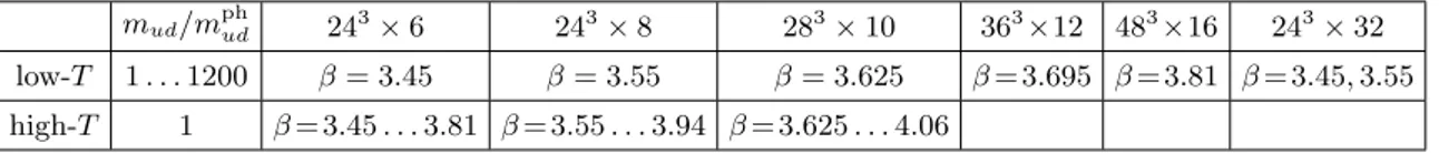
mud/mphud 243×6 243×8 283×10 363×12 483×16 243×32 low-T 1. . .1200 β= 3.45 β= 3.55 β= 3.625 β= 3.695 β= 3.81 β= 3.45,3.55 high-T 1 β= 3.45. . .3.81 β= 3.55. . .3.94 β= 3.625. . .4.06
Table 1. Summary of our lattice ensembles.
3.4 Lattice ensembles
Before presenting the results, we briefly describe the lattice ensembles we used. These consist of two sets of lattice configurations: one at high temperatures, necessary for the determination of the T-dependence of the EoS, and one at effectively zero temperature, necessary for the renormalization. The high-T ensemble containsNt= 6, 8 and 10 lattices with various values of the inverse gauge coupling β, such that the temperature range 113 MeV< T < 300 MeV can be scanned and a continuum estimate can be given (note that at a fixed temperature, the lattice spacing is proportional to 1/Nt such that the continuum limit corresponds to Nt → ∞, see eq. (3.1)). These configurations correspond to physical quark masses, tuned along the LCP as discussed at the beginning of section3.
This ensemble was mainly generated in ref. [16] for the study of the phase diagram and is supplemented in the present analysis by configurations atT = 250 MeV andT = 300 MeV.
Based on detailed comparisons to our zero-temperature 243×32 ensembles (see sec- tion 4.2), it turned out that the renormalization factors can be determined reliably at our lowest ‘finite-temperature’ point, T = 113 MeV. At this temperature we included two additional lattice spacings withNt= 12 and 16, allowing for a determination of the renor- malization factors down to small lattice spacings, and a matching with perturbation theory.
For eachNt we generated configurations ranging frommud=mphud up tomud= 1200·mphud. The simulation parameters are listed in table1.
4 Results
4.1 Condensates, the β-function and a comment on magnetic catalysis
We start the presentation of our results with additional details on and implications of the generalized integral method. Let us consider the integrand on the right hand side of eq. (3.22), and expand it in powers of eB. For asymptotically large quark masses, quarks and gluons decouple, and ∆ ¯ψfψf approaches its free theory value. In this limit, we obtain from eq. (3.11),
P[mf·∆ ¯ψfψfreef ]
(eB)2 =bfree1f , (4.1)
whereP is the projector defined in eq. (3.20). In figure2we plotP[mud∆ ¯ψdψd] normalized by (eB)2 as a function of the light quark mass at T = 113 MeV. We perform a combined continuum extrapolation of all five lattice spacings (Nt = 6,8,10,12 and 16), assuming O(a2) discretization errors. The plotted combination has a finite continuum limit (see the discussion after eq. (3.16)), but discretization errors become large when the lattice quark mass muda approaches unity. For asymptotically large masses the change of the
JHEP08(2014)177
Figure 2. TheO((eB)2) contribution to the integrand of eq. (3.22) normalized by (eB)2 for five different lattice spacings and the continuum extrapolation. The free theory prediction (dashed line) and the expectation fromχPT (dashed-dotted line) are also shown. For asymptotically large quark masses (muda= 1 for each lattice spacing is marked by the colored bars in the upper right corner) lattice artefacts become large andP[mud∆ ¯ψdψd] drops.
condensate is proportional to (muda)−5, as shown in appendix A. The finer the lattice, the later this lattice artefact sets in, and the larger are the quark masses that can be reached. With our present lattice spacings we can control the continuum extrapolation up tomud/mphud ≈100−200. Here the extrapolated values are consistent with the free theory prediction, eq. (4.1), showing that in the continuum limit ∆ ¯ψfψf ∝1/mf for large masses mf ΛQCD, to quadratic order in eB. This implies that the O((eB)2) contribution to the integral on the right hand side of eq. (3.22) diverges logarithmically. On the lattice this divergence is regulated by the inverse lattice spacing such that the cutoff mfa ≈ 1 plays the role of the upper limit of the mass-integral, see the sharp drop in figure 2 for asymptotically large masses mf &a−1. In the continuum limit the logarithmic divergence reappears (cf. eq. (3.15)), and has to be subtracted via charge renormalization.
Let us now determine the chiral limit of the combination shown in figure2using chiral perturbation theory (χPT). The lowest excitation in this case is the charged pion, implying that to leading order ΛH =mπ in eqs. (3.15) and (3.16). Moreover, due to the spin-zero nature of the pion, the scalar QED β-function appears instead of the spinor β-function.
Using the Gell-Mann-Oakes-Renner relation m2πF2 = ¯ψψ(0)(mu+md) we obtain for the light flavorsf =u, d,
mf
m2π ·∂m2π
∂mf = 1
2, P[mf ·∆ ¯ψfψχPTf ]
(eB)2 = bfree,scalar 1f
4Nc = bfree1f
16Nc, (4.2) as was already pointed out within the Hadron Resonance Gas (HRG) model [32]. To derive eq. (4.2), we considered equal masses for the light flavors mu = md. Note that the first relation in eq. (4.2) is understood to hold at B = 0, where the charged and neutral pion masses are equal. We indicate the χPT prediction in figure 2 by the dashed-dotted line, showing a good agreement with the lattice data at physical quark masses, see also the comparison in ref. [39].
JHEP08(2014)177
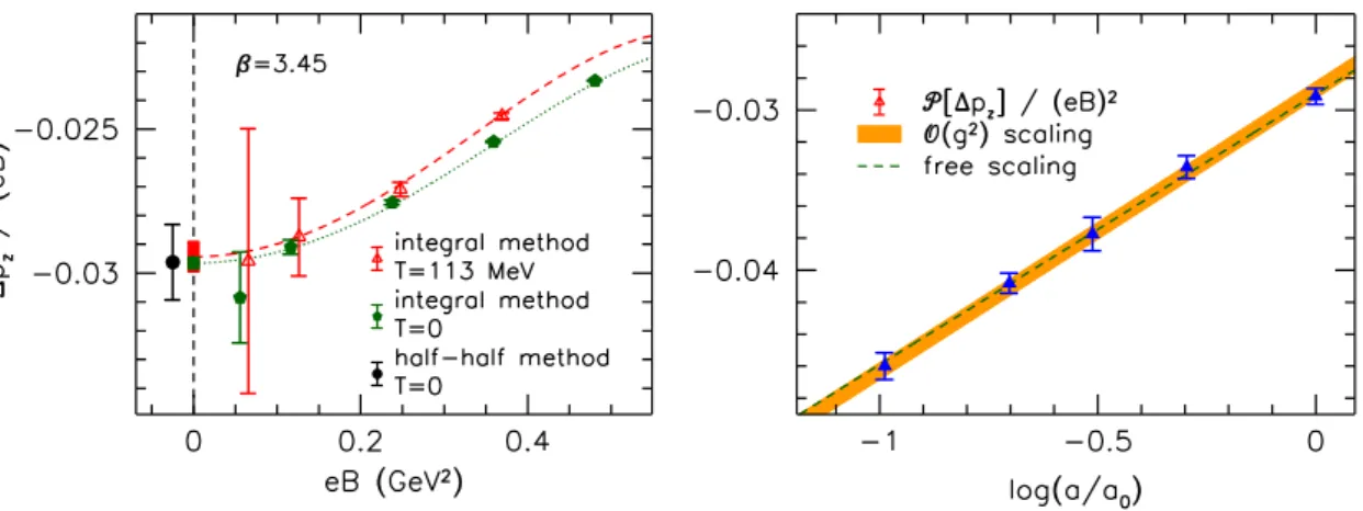
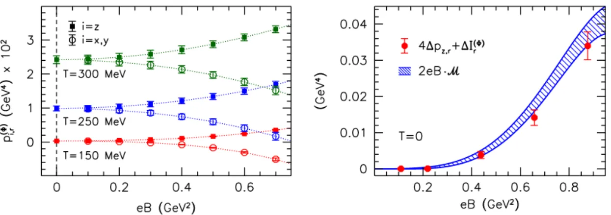
Figure 3. Left panel: magnetic field-dependence of the bare longitudinal pressure difference at low temperatures at one lattice spacing. The results of the integral method atT = 113 MeV and at T = 0, and the result of the half-half method atT = 0 are compared (the points are slightly shifted horizontally for better visibility). Right panel: quadratic contribution to the bare longitudinal pressure atT = 113 MeV against the lattice spacing in units ofa0= 1.47 GeV−1.
Altogether we observe that the QCD quark condensate, as determined in a fully non- perturbative treatment, interpolates between theχPT prediction at small masses and the free-theory limit at large masses. We have seen in eq. (3.16) that the sign of the condensate
∆ ¯ψfψf equals the product of the sign of the factor ∂ΛH/∂mf and that of b1. While for large quark masses mf ΛQCD one has ΛH = mf, towards the chiral limit ΛH = mπ such that the first factor is in both cases positive. It would be quite unexpected to have an intermediate mass where this factor turned negative, nevertheless, we did not find any strict proof of this positivity. In any case we conclude that the O((eB)2) magnetic catalysis of the quark condensate and the positivity of the scalar/spinor QED β-function are intimately related phenomena. This picture was first described in ref. [32] and also discussed in ref. [27]. Note that the above argument concerns theO((eB)2) behavior of the condensate and does not address what happens in the large-B limit, where the dimensional reduction is expected to be the dominant driving force of magnetic catalysis [34].
4.2 Quadratic contribution to the EoS
Next we calculate theO((eB)2) contribution to the longitudinal pressure at effectively zero temperature. This term will be subtracted through charge renormalization, according to eq. (3.19). We perform the integral eq. (3.22) to determine ∆pz at various values of the magnetic flux (see the left panel of figure 3). To extract the O((eB)2) contribution, we fit the data to a quadratic function in (eB)2 and take the B → 0 limit of ∆pz/(eB)2, represented by the bars at eB = 0 in the figure. We perform this analysis for the 243× 6 ensemble at our lowest finite-temperature point, T = 113 MeV, and on the 243 ×32 ensemble, which corresponds to T = 0. The B → 0 limits at these two temperatures are found to coincide within our statistical errors. This implies that thermal contributions to the O((eB)2) pressure are still strongly suppressed at T = 113 MeV, in agreement with our previous findings from the anisotropy method [18], with the results of ref. [24] using
JHEP08(2014)177
the half-half method and with those of ref. [26] using the finite difference method (for a brief description of these approaches, see section3.1). Therefore, we conclude that within our present statistics, it is safe to use T = 113 MeV as the reference temperature for the quadratic subtraction. This observation allows us to omit expensive lattice simulations at T = 0, and to substitute these by cheaper runs at a finite but low temperature.
In addition, we also check the eB → 0 extrapolation of our results by directly deter- mining the second derivative of ∆pz with respect to the magnetic field at eB = 0 using the half-half method atT = 0. For this measurement we employ the setup of ref. [24] and use 400 noisy estimators to calculate the trace of the necessary operators (for details see ref. [24]). The result is indicated by the black point in the left panel of figure 4, showing that the two methods agree perfectly. Note that in the generalized integral method we use results at all B >0 to extract the quadratic part, resulting in smaller errors. Increasing instead the statistics atB = 0 for the half-half method, we could also improve the signal- to-noise ratio of the latter, however finite volume effects should also be studied carefully in this case. Since the results at eB > 0 will be in any case necessary for calculating the higher order contributions to the renormalized pressure, it is advantageous to use the generalized integral method to extract the quadratic term as well.
We proceed by discussing the dependence of P[∆pz] ona. First we perform theB →0 extrapolation separately for each of our five lattice spacings. The resulting values are expected to lie on the curve b1(a) ·log(ΛHa), see eq. (3.15). We consider the universal one-loop QCD corrections to b1(a) — i.e. terms up to i = 1 in eq. (3.14). The strong coupling in the lattice scheme is defined as g2(1/a) = 6/β(a). The so obtained function b1(a)·log(ΛHa) is fitted to the data with ΛHconsidered as a free parameter. The result is indicated by the orange band in the right panel of figure 3. For comparison we also carry out a similar fit in the free case, which corresponds to a simple linear fit with fixed slope bfree1 = 0.0169 (which is obtained using eq. (3.9) for three flavors). The two fits agree within errors for the whole range, indicating that for our lattice spacings, the QCD corrections to the QEDβ-function in eq. (3.14) are smaller than our statistical errors.
Exploiting the fact that the free scaling describes our data to a very good accuracy, we consider an alternative strategy to determine the quadratic contribution to ∆pz. Namely, we fit the results for ∆pz/(eB)2 at all magnetic fields and lattice spacings together using a combined inter/extrapolation inaand eB. We consider the fit function
∆pz
(eB)2 =c0+bfree1 log (a/a0) + (eB)2· c1+c01a2+c001a4
+ (eB)4· c2+c02a2
, (4.3) which takes into account the logarithmic divergence of the constant term (with the free scaling coefficient). Here a0 = 1.47 GeV−1 is our largest lattice spacing (corresponding to Nt= 6). We found it necessary to include O(a4) lattice discretization effects in the (eB)2 part and O(a2) terms in the (eB)4 part of the fit function. The results of this combined fit are shown in the left panel of figure 4. Considering higher orders in the magnetic field or more lattice artefacts in eq. (4.3) did not improve the quality of the fit. The eB → 0 limits (colored bars in the figure) equal P[pz]/(eB)2, giving the logarithmically divergent termc0+bfree1 log(a/a0) that is subtracted via charge renormalization, as a function of the
JHEP08(2014)177
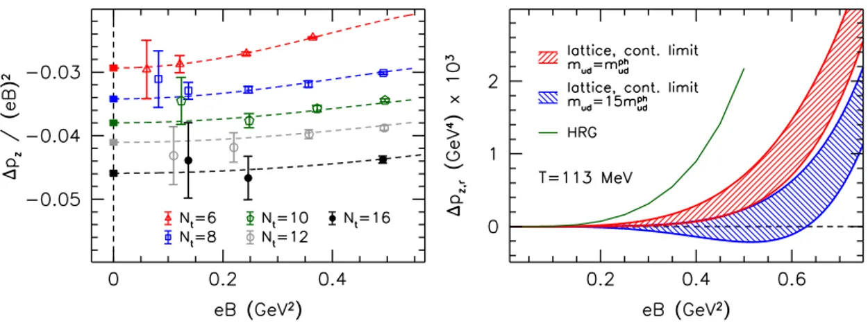
Figure 4. Left panel: combined extrapolation in the magnetic field and interpolation in the lattice spacing according to eq. (4.3) using several values of the magnetic flux and five lattice spacings.
Only data points witheB <0.5 GeV2are shown. Right panel: continuum limit of the renormalized magnetization for physicalmud=mphud(red dashed band) and heavier-than-physicalmud = 15·mphud quark masses (blue dashed band), and a comparison to the HRG model.
c0 c1 c01 c001
−0.0294(5) 0.006(6) GeV−4 0.011(7) GeV−2 0.003(2)
c2 c02 bfree1 a0
0.007(8) GeV−8 −0.025(9) GeV−6 0.0169 1.47 GeV−1 Table 2. Parameters of the fit function eq. (4.3).
lattice spacing. The fitted coefficients are listed in table2. As a cross-check we carried out a similar fit withb1 as a free parameter, resulting in a value consistent with the expected continuum value bfree1 . Matching eq. (4.3) with eq. (3.15) we read off that at the physical value of the quark masses
ΛH(mphud) =ec0/bfree1 /a0 = 0.120(9) GeV. (4.4) The scale ΛH depends on the regularization scheme (i.e. on the lattice action). However, towards the chiral limit it is expected to approach a hadronic scale, ΛχPTH =mπ (see the discussion in section 4.1), so that this scheme-dependence should only be mild. We stress that ΛHis no free parameter but is automatically determined by the lattice implementation of the renormalization prescription eq. (3.19). ΛH will appear below in the perturbative description of the pressure as an input from the lattice side.
Subtracting terms quadratic ineBgives the renormalized pressure ∆pz,r= (1−P)[∆pz] atT = 113 MeV. Its continuum limit is given by thea→0 limit of our fit function eq. (4.3) and is shown in the right panel of figure 4. Note that the positivity of ∆pz,r indicates the response to be paramagnetic. Besides the curve for the physical quark masses, we also include here the results obtained for heavier-than-physical quark masses. The analysis is the same in this case except for the lower endpoint of the integral in eq. (3.22) which we set to mud = 15·mphud. These light quark masses correspond to a pion mass of about
JHEP08(2014)177
Figure 5. Longitudinal pressure (left panel) and interaction measure in the Φ-scheme (right panel), normalized by T4 as functions of the temperature, measured on our Nt= 6 ensemble. Both pz,r
andIr(Φ)are nonzero atT = 0, which shows up as a quartic divergence atT = 0.
500 MeV, and the fit according to eq. (4.3) gives ΛH(15mphud) = 159(10) MeV. The plot shows that the pressure is clearly less sensitive onBas quarks become heavier. In addition we also indicate the Hadron Resonance Gas (HRG) model prediction [32] for the physical pion mass. We will get back to the visible discrepancy between the lattice results and the model curve in section4.3below.
4.3 Complete magnetic field dependence of the EoS
With the quadratic contribution determined as a function of the lattice spacing, we can carry out the renormalization of the pressure according to eq. (3.19), and that of the interaction measure using eq. (3.18) for arbitrary temperatures. Using these two renormal- ized observables, all other EoS-related quantities can be calculated via the thermodynamic relations of section 2.
At B = 0 the usual normalization of, e.g., the pressure is p/T4. In our case this may not be the optimal choice, since pcontains terms of O((eB)4) at zero temperature, which give rise to a∼1/T4divergence towardsT = 0. We demonstrate this in figure5for the case of the longitudinal pressure (left panel) and the interaction measure in the Φ-scheme (right panel). It is therefore instructive to plot the observables without this normalization with respect to T4. First we show the change in the EoS induced by the magnetic field, ∆pz,r
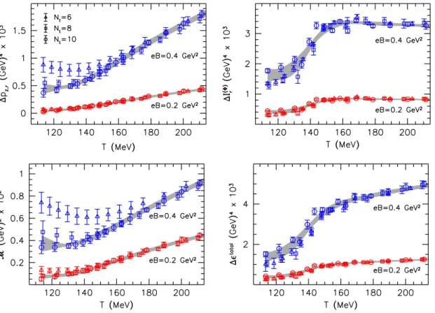
and ∆Ir(Φ)for two values ofeB, see figure6. We find that in the low-temperature region our three lattice spacings do not suffice to perform a controlled continuum extrapolation.5 To allow for a parameterization of our results we consider a continuum estimate as the average of ourNt= 8 andNt= 10 results. This estimate is indicated by the gray shaded bands in the figures and is used in the following analysis. Note the positivity ofM, which indicates the paramagnetic nature of the thermal QCD medium for the whole temperature range.
5A well-known source of lattice artefact is the taste symmetry breaking of staggered fermions, which may lead to large discretization effects at low temperatures. Note that not all observables are affected equally by these artefacts.
JHEP08(2014)177
Figure 6. Change in the EoS due to the magnetic field. Shown are the longitudinal pressure (upper left panel), the Φ-scheme interaction measure (upper right panel), the magnetization (lower left panel) and the energy density (lower right panel) as functions of the temperature for three lattice spacings and two values of eB. The shaded areas correspond to our continuum estimates (see the text).
We proceed by discussing the full EoS at nonzero magnetic fields and concentrate on the low-temperature region where the HRG model is expected to be a valid description.
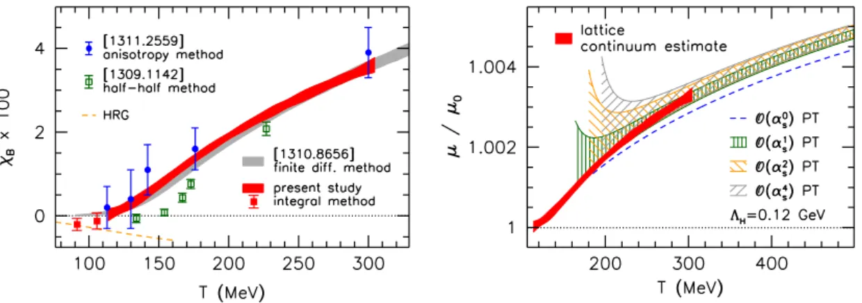
In figure 7 we show the longitudinal pressure and the ratio of pressure over total energy density. Comparing pz,r with the HRG model reveals that the model overestimates the pressure at nonzero magnetic fields. This mismatch between the model and the lattice results was not yet visible in our previous comparison [27], where only the Nt= 6 lattice data were available. The ratiopz,r/total(see eq. (2.1) for our definition oftotal) exhibits a shallow dip in the transition region, which moves towards the left, signaling the reduction of the transition temperature as B grows, in accordance with our earlier findings with other thermodynamic observables [16,17]. This dip is, however, not pronounced enough to enable us to reliably determine the position of its minimum. We will study the dependence of the transition temperature on B in section 4.6.
Up to now we only discussed the longitudinal pressure. Depending on which scheme is used, the magnetic field can induce an anisotropy between the pressure components, see eq. (2.4). The Φ-scheme describes a situation, in which the transverse compression of the system proceeds at fixed magnetic flux, thereby inducing an anisotropy that is proportional