The Vapor Pressure of Mercury

(1)

The Vapor Pressure of Mercury

Marcia L. Huber Arno Laesecke Daniel G. Friend

NISTIR 6643

(2)

NISTIR 6643

The Vapor Pressure of Mercury

Marcia L. Huber Arno Laesecke Daniel G. Friend

Physical and Chemical Properties Division Chemical Science and Technology Laboratory National Institute of Standards and Technology Boulder, CO 80305-3328

April 2006

U.S. DEPARTMENT OF COMMERCE Carlos M. Gutierrez, Secretary TECHNOLOGY ADMINISTRATION Robert Cresanti, Under Secretary of Commerce for Technology NATIONAL INSTITUTE OF STANDARDS AND TECHNOLOGY William Jeffrey, Director

(3)

Table of Contents

1. Introduction...1

2. Experimental Vapor Pressure Data ...2

3. Correlation Development...11

4. Comparison with Experimental Data...18

5. Comparisons with Correlations from the Literature...23

6. Detailed Comparisons for the Temperature Range 0 °C to 60 °C...25

7. Conclusions...35

8. References...36

Appendix A: Detailed Listing of Experimental Data for the Vapor Pressure of Mercury...42

Appendix B: Detailed Listing of Supplemental Experimental Data for the Heat Capacity of Mercury...56

(4)

The Vapor Pressure of Mercury

Marcia L. Huber, Arno Laesecke, and Daniel G. Friend National Institute of Standards and Technology∗

Boulder, CO 80303-3328

In this report, we review the available measurements of the vapor pressure of mercury and develop a new correlation that is valid from the triple point to the critical point. The equation is a Wagner-type form, where the terms of the

equation are selected by use of a simulated annealing optimization algorithm. In order to improve the reliability of the equation at low temperatures, heat capacity data were used in addition to vapor pressure data. We present comparisons with available experimental data and existing correlations. In the region of interest for this project, over the temperature range 0 °C to 60 °C, the estimated uncertainty (estimated as a combined expanded uncertainty with coverage factor of 2, 2σ) of the correlation is 1 %.

Keywords: correlation, mercury, vapor pressure.

1. Introduction

Recent concerns about mercury as an industrial pollutant have lead to increased interest in the detection and regulation of mercury in the environment [1]. The

development of standardized equations for the thermophysical properties of mercury can aid this task. A critical evaluation of density, thermal expansion coefficients, and

compressibilities as a function of temperature and pressure was conducted by Holman and ten Seldam [2]. Bettin and Fehlauer [3] recently reviewed the density of mercury for metrological applications. Vukalovich and Fokin’s book [4] and the Gmelin Handbook [5] are both thorough treatises on the thermophysical properties of mercury. Thermal properties such as thermal conductivity and heat capacity were reviewed by Sakonidou et al. [6], while Hensel and Warren [7] cover other properties including optical and

magnetic characteristics. To assess risks of exposure, it is important to have an accurate

∗ Physical and Chemical Properties Division, Chemical Science and Technology Laboratory.

(5)

representation of the vapor pressure of mercury. Numerous compilations and correlations of the vapor pressure of mercury have been published [8-25], but there is no consensus on which is the best one to use for a given purpose. In this work, we review the existing experimental data and correlations, and provide a new representation of the vapor pressure of mercury that is valid from the triple point to the critical point. We also present comparisons with both experimental data and correlations, and estimate the uncertainty of the correlation.

2. Experimental Vapor Pressure Data

Experimental measurements of the vapor pressure of mercury have a long history.

A single vapor pressure point of mercury, the boiling point, was first measured in 1801 by Dalton [26], who obtained a value corresponding to 622 K; shortly thereafter, in 1803, Crichton [27] mentioned that the normal boiling point is above a temperature

corresponding to 619 K. More recently, the normal boiling point of mercury was determined by Beattie et al. [28] as (356.58 ± 0.0016) °C, on the 1927 International Temperature Scale. This measurement was selected as a secondary fixed point on the ITS-48 Temperature scale [29]. Converted to the ITS-90 temperature scale [30], this value is (629.7653 ± 0.0016) K. The value recommended by Marsh [31] is 629.81 K (IPTS-68); on the International Practical Temperature Scale [32] of 1968, this was a secondary fixed point. Converted to ITS-90, this recommendation is 629.7683 K for the normal boiling point.

Regnault [33] published observations of the vapor pressure of mercury over a range of temperatures in 1862. Several of the early publications are by researchers who became quite famous, including Avogadro [34], Dalton [26], Hertz [35], Ramsay [36], and Haber [37]. Indeed, much of the work on mercury was done in the early part of the 20th century. Figure 1 shows the distribution of the experimental data. Table 1 gives a detailed compilation of sources of vapor-pressure data from 1862 to the present, along with the temperature range of the measurements, the experimental method used, and an estimate of the uncertainty of these measurements. In general, determinations of the purity of the mercury were not available; however, methods for the purification of

(6)

before it was possible to quantify the purity [18]. The estimates of uncertainty were obtained by considering the experimental method and conditions, the original author’s estimates (when available), and agreement with preliminary correlations. These

correspond to our estimate of a combined expanded uncertainty with a coverage factor of two. In Appendix A, we tabulate all experimental data for the vapor pressure of mercury collected in this study.

The experimental techniques used to measure vapor pressure can be grouped into three main categories: the static, quasistatic, and kinetic techniques are discussed by Dykyj et al. [38] and Ditchburn and Gilmour [14]. One of the simplest methods to measure the vapor pressure is a static method that involves placing the sample in a closed container, then removing any air and impurities, keeping the vessel at constant

temperature, and then measuring the temperature and pressure after equilibrium has been established. It is generally limited to pressures above 10 kPa. In principle, it is applicable to any pressure, but in practice the presence of nonvolatile impurities can cause large systematic errors. With very careful sample preparation, it may be possible to go to lower pressures with this technique. Another static instrument is the isoteniscope. This type of instrument was used by Smith and Menzies [39, 40] in their early work on the vapor pressure of mercury. In this type of apparatus, the sample is placed in a bulb that is connected to a U-tube that acts as a manometer (i.e., a pressure sensor). The device is placed in a thermostat, and the external pressure is adjusted until it equals that of the vapor above the sample. Isoteniscopes are limited by the sensitivity of the pressure sensor. A third type of static method involves the use of an inclined piston gauge. The sample is placed in a cylinder fitted with a movable piston so that the pressure of the sample balances the weight (gravitational force) of the piston. This method is generally applicable over the range 0.1 kPa to 1.5 kPa.

Among the instruments classified as quasistatic are ebulliometers and

transpiration methods. In both of them, a steady rate of boiling is established, and it is assumed that the pressure at steady state is equivalent to the equilibrium vapor pressure.

In an ebulliometer, the sample is boiled at a pressure set by an external pressurizing gas (often helium) with the vapor passing through a reflux condenser before returning to the boiler. The temperature measured is that of the vapor just above the boiling liquid. An

(7)

advantage to this method is that volatile impurities do not condense and are removed at the top of the apparatus. This method may also be set up in a comparative mode with two separate ebulliometers, one containing a reference fluid and the other containing the sample fluid connected with a common pressure line, so that direct measurement of the pressure is unnecessary. It is possible to make very accurate measurements with this type of device, at pressures greater than about 2 kPa. The very accurate measurements of the vapor pressure of mercury by Ambrose and Sprake [18] were made with an ebulliometric technique. The transpiration method (also called gas saturation) involves passing a steady stream of an inert gas over or through the sample, which is held at constant temperature.

The pressure is not measured directly, but rather is calculated from converting the concentration of the mercury in the gas stream to a partial pressure that is the vapor pressure of the sample. This type of method has a larger uncertainty than some of the other methods, generally ranging from 0.5 to 5 % [38]. It is most useful over a pressure range of 0.1 to 5 kPa. For example, Burlingame [43] and Dauphinee [49,50] used the transpiration method in their measurements.

(8)

1E-9

1E-6

1E-3

1E+0

1E+3

1E+6 1003005007009001100130015001700 Temperature, K

Pressur e, kPa

Regnault 1862 Hertz 1882 Ramsay 1886 Callendar 1891 Young 1891 Cailletet 1897 Pfaundler 1897 Morley 1904 Gebhardt 1905 Smith, Menzies 1910, 1927 Knudsen 1909 Egerton 1917 Ruff 1919 Volmer 1921 Hill 1922 Scott 1924 Bernhardt 1925 Poindexter 1925 Rodebush 1925 Volmer1925 Jenkins 1926 Millar 1927 Neumann 1932 Pedder 1933 von Halban 1935 Beattie 1937 Schneider 1944 Dauphinee 1950 Douglas 1951 Busey 1953 Ernsberger 1955 Spedding 1955 Roeder 1956 Sugawara 1962 Carlson 1963 Schmahl 1965 Morgulescu 1966 Ambrose 1972 Schönherr 1981 Triple point Normal boiling point Critical point Figure 1. Experimental vapor pressure data for mercury. 5

(9)

mary of available data for the vapor pressure of mercury. References in boldface indicate primary data sets (see text). Year Method No. pts. T range, K Estimated uncertainty, % 1972 ebulliometer 113 417-771 less than 0.03, greatest at lowest T 1937boiling tube42623-6360.03 1925 3 static methods 27 694-1706 varies from 2 to >15 1881 Töpler vacuum pump 2 273-293 >20 e [43] 1968 transpiration 38 344-409 4 1953 derived from caloric properties 24 234-750 varies from 0.2 to 3.5 at lowest T 1900 Bourdon manometer 11 673-1154 varies from 1 to 7 1891 Meyer tube 2 630 0.2 menga [47] 1969 effusion graphical results 273-325 1963 effusion 9 299-549 varies from 3 to >20 1950,1951 transpiration 18 305-455 5 1951 derived from caloric properties 30 234-773 varies from 0.03 (at normal boiling point) to 1.5 at lowest T 1920 gives table attributed to Smith and Menzies[39] 46273-723 1917 effusion 27 289-309 5 1955piston manometer18285-3271 1978 static method graphical results 523-723 3 1984 atomic absorption correlating equation only 723-8733 1905 boiling tube 9 403-483 8 1914 vibrating quartz filament 1 293 2 1882 differential pressure 5 273-473 >20 1966 electrical resistance graphical results 1073-critical not available 1882 static absolute manometer 9 363-480 5 1913 not available 1 630 0.2 1964 torsion-effusion 6 295-332 5 1922 radiometer principle 19 272-308 30 1982 static graphical results 742-1271 not available 1926 isoteniscope 21 479-671 0.1 to >20 [65] 1894 ebulliometer 43 393-493 >10 1909 effusion 10 273-324 varies from 5 to 10 1910 radiometer principle 7 263-298 varies from 5 to 10 6

(10)

Table 1. Continued. First Author Year Method No. pts. T range, K Estimated uncertainty, % Kordes [68] 1929 temperature scanning evaporation method 2 630-632 4 Mayer [69] 1930 effusion 82 261-298 5, except greater at T<270 McLeod [70] 1883 transpiration 1 293 >20 Menzies [39, 40] 1910,1927 isoteniscope46395-7080.5 Millar [71] 1927 isoteniscope 6 468-614 2 Morley [72] 1904 transpiration 6 289-343 varies from 8 to >20 Murgulescu [73] 1966 quasi-static 9 301-549 3 Neumann [74] 1932 torsion balance 19 290-344 6 Pedder [75] 1933 transpiration 3 559-573 2 Pfaundler [76] 1897 gas saturation 3 288-372 12 Poindexter [77] 1925 ionization gage 17* 235-293 5-20, greatest at lowest T Raabe [78] 2003 computer simulation 20 408-1575 varies from 0.5 to >20 Ramsay [36] 1886 isoteniscope 13 495-721 varies from 0.3 to 10 at highest T Regnault [33] 1862 isoteniscope 29 297-785 ~6 for T>400, much higher for lower T Rodebush [79] 1925 quasi-static 7 444-476 1 Roeder [80] 1956 quartz spiral manometer 7 413-614 2 Ruff [81] 1919 temperature scanning evaporation method 12478-630 >20 Schmahl [82] 1965 static method 43 412-640 1.5 Schneider [83] 1944 gas saturation 23 484-575 10 Schönherr [84] 1981electrical conductivity131052-17353 Scott [85] 1924 vibrating quartz filament 1 293 2 Shpil’rain [86] 1971 ebulliometer 50 554-883 0.6 to 0.8 Spedding [87] 1955isoteniscope13534-6300.03 Stock [88]* 1929 transpiration 3 253-283 20 Sugawara [9] 1962 static method 14 602-930 2 van der Plaats [89] 1886 transpiration 26 273-358 Villiers [90] 1913 ebulliometer 12 333-373 6 Volmer [91] 1925 effusion 10 303-313 3 von Halban [92] 1935 resonance light absorption 1* 255 7 Young [93] 1891 static 11 457-718 2 * Excludes points below the triple point. 7

(11)

The Knudsen effusion method is a type of vapor pressure measurement classified as a dynamic method. In this type of experiment, a steady rate of evaporation through an orifice into a vacuum is established, and pressure is calculated from the flow rate through the orifice by use of kinetic theory. This method is applicable at very low pressures (below 0.1 kPa), but generally has high uncertainties.

As indicated in Table 1, many measurements have been made on the vapor pressure of mercury. However, only a limited number of these are comprehensive and have

uncertainty levels of one percent or less. These sets have been identified as primary data sets in our work and are indicated by boldface type in Table 1. In general, the most accurate measurements were those made with ebulliometric methods. Ambrose and Sprake [18] used an ebulliometric technique for their measurements from 380 K to 771 K. These data have an uncertainty of about 0.03 % or lower, with the largest uncertainty at the lowest temperatures.

Beattie et al. [28] very accurately determined the boiling point of mercury over the

temperature range 623 K to 636 K. Spedding and Dye [87] used an isoteniscope to measure the vapor pressure over the range 534 K to 630 K, with uncertainties on the order of 0.03 % except at the lowest temperatures where they are larger. Menzies [40, 94] used an

isoteniscope at temperatures from 395 K to 708 K, but these data show more scatter and have larger uncertainties than the sets mentioned above; however, the uncertainties are still less than 0.5 %. Shpil’rain and Nikanorov [86] used an ebulliometric method extending from 554 K to 883 K. Their data are more consistent with the measurements of Ambrose and Sprake [18] in their region of overlap than are other high temperature sets, such as those by

Sugawara et al. [9] , Bernhardt [41] or Cailletet et al. [45], and thus were selected as the primary data for the high temperature region from about 700 K to 900 K. In addition, although the uncertainty is higher than 1 %, we have selected the data of Schönherr and Hensel [84] for the highest temperature region, 1052 K to 1735 K. This data set was obtained by observing changes in the electrical conductivity. At fixed pressures, the temperature was raised, and when a discontinuity was observed, this was taken as an indication of phase change.

All of the sets mentioned so far are for temperatures greater than 380 K. At lower temperatures, the measurements are much more uncertain and display significant scatter. In

(12)

to be the most accurate. These measurements were made with an absolute manometer method, with uncertainties on the order of 1 %, and they cover the temperature range 285 K to 327 K. This data set has been adopted in the metrology community for use in precision manometry, and has been described as reliable and confirmed by heat capacity measurements [95]. The reliability and thermodynamic consistency of these data will be discussed in more detail in a later section of this document.

The end points of the vapor pressure curve for stable vapor-liquid equilibrium are the triple point and the critical point. Metastable points may be obtained at points below the triple point. In principle, the three phase-boundary curves that meet at the gas-liquid-solid triple point of a pure substance continue beyond this intersection so that the phase equilibria become metastable relative to the third phase, which is absolutely stable. Vapor-liquid equilibrium along the vapor pressure curve continued below the triple point becomes metastable relative to the solid phase, and vapor-solid equilibrium along the sublimation pressure curve continued above the triple point becomes metastable relative to the liquid phase. Although the former has been realized in experiments [96], metastable phase equilibria are one of the least investigated phenomena of the behavior of matter. Their existence in principle is mentioned here because three datasets in the present collection report mercury vapor pressure data at temperatures below the triple point: Poindexter [77], Stock and Zimmermann [88], and von Halban [92]. The farthest reaching data below the triple point temperature are the results of Poindexter, covering a range from 194 K to 293 K.

However, in this work we restrict our study to points above the triple point, although all points are tabulated in Appendix A.

The triple point of mercury has been designated as a fixed point of the ITS-90 [30]

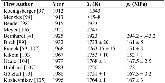
temperature scale, with a value of 234.3156 K. The critical point has been measured by several investigators; these values are listed in Table 2, along with uncertainty estimates provided by the authors. One of the first measurements of the critical point was made by Koenigsberger [97] in 1912, who made visual observations in a quartz tube and reported the critical temperature of mercury to be near 1270 °C (1543 K). This measurement was later criticized by Menzies [94] who reported that the critical temperature was at least 1275 °C (1548 K). Another early determination was that of Bernhardt [41] who extrapolated his vapor pressure observations, and used Bender’s [98] value of 1650 °C (1923 K) for the critical

(13)

temperature, while estimating the critical pressure to be in the range 294.2 to 343.2 MPa.

Later, Birch [99] determined the critical point by observing the changes in electrical resistance as a function of temperature at constant pressure. The review paper of Mathews [100] adopted Birch’s values for the critical point. Ambrose [101] and also Vargaftik et al.

[8] instead selected the value obtained by Franck and Hensel [102], also obtained from studies of changes in electrical resistance. Kikoin and Senchenkov [103] used electrical conductivity experiments to locate the critical point, Neale and Cusack [104] observed changes in the Seebeck voltage, while Götzlaff [13] analyzed isochoric and isobaric PVT data extrapolated to the saturation boundary. Most recently Kozhevnikov et al. [105]

observed changes in the speed of sound along isobars as a function of temperature to determine the critical point. The value by Bernhardt [41] is too high both in pressure and in temperature. The critical temperature of Franck and Hensel [102] agrees very well with that obtained by Kozhevnikov et al. [105], while the critical pressure of Götzlaff [13] agrees very well with that of Kozhevnikov et al. [105] In this work we adopted the critical point of Kozhevnikov et al. [105].

Table 2. The critical temperature and pressure of mercury.*

First Author Year Tc (K) pc (MPa) Koenigsberger [97] 1912 ~1543

Menzies [94] 1913 >1548

Bender [98] 1915 1923

Meyer [106] 1921 1747

Bernhardt [41] 1925 1923 294.2 - 343.2

Birch [99] 1932 1733 ± 20 161 ± 5

Franck [59, 102] 1966 1763.15 ± 15 151 ± 3

Kikoin [103] 1967 1753 ± 10 152 ± 1

Neale [104] 1979 1768 ± 8 167.5 ± 2.5

Hubbard [107] 1983 1750 172

Götzlaff [13] 1988 1751 ± 1 167.3 ± 0.2

Kozhevnikov [105] 1996 1764 ± 1 167 ± 3

*Uncertainties are expressed in kelvins and megapascals for the temperature and pressure, respectively.

(14)

3. Correlation Development

Numerous expressions have been used to represent the vapor pressure of a pure fluid;

many are reviewed in Růžička and Majer [108]. Equations of the general form

( / _c) ( / )_c _i ⁱ/ 2 i

ln p p = T T

∑

aτ ^, (1) where τ = 1-T/Tc, are attributed to Wagner [109-112] and have been used successfully to represent the vapor pressures of a wide variety of fluids. Lemmon and Goodwin [113] used the Wagner form with exponents (1, 1.5, 2.5, and 5) to represent the vapor pressures of normal alkanes up to C36. This form, which we will call Wagner 2.5-5, is one of the most widely used forms along with the equation with exponents (1, 1.5, 3, and 6) [109, 110], which we call Wagner 3-6. The 2.5-5 form has emerged as the generally preferred form [114]. When the data set is extensive and of high quality, other forms with alternative sets of exponents with additional terms have been used. For example, a Wagner equation with exponents (1, 1.5, 2, 2.5, and 5.5) was used to represent the vapor pressure of acetonitrile [115], and another variant of the Wagner equation, with exponents (1, 1.89, 2, 3, and 3.6), was used to represent the vapor pressure of heavy water [116] from the triple point to the critical point to within the experimental scatter of the measurements. The International Association for the Properties of Water and Steam (IAPWS) formulation for the vapor pressure of water [117, 118] uses a six-term Wagner equation with exponents of (1, 1.5, 3, 3.5, 4, and 7.5).

Since there is a lack of high-quality experimental vapor-pressure data in the low temperature region (T < 285 K), liquid heat capacity measurements at low temperatures can be used to supplement the vapor-pressure data [108, 114, 119]. This permits the

simultaneous regression of heat capacity and vapor-pressure data to determine the

coefficients of a vapor pressure equation that is valid down to the triple point. An alternative method is to use an expression involving enthalpies of vaporization in addition to vapor- pressure data [120]. Both of these approaches can be used to ensure that the vapor pressure is thermodynamically consistent with other thermodynamic data.

King and Al-Najjar [119] related heat capacity and vapor pressure using

(15)

0

2 dlnp_sat C_p C_p^L G

d T

dT dT R

− −

⎛ ⎞ =

⎜ ⎟

⎝ ⎠ , (2)

·K), psat is the vapor ressure, and G represents vapor phase nonidealities and is given by

where Cp° and CpL are the heat capacities at constant pressure of the ideal gas and the saturated liquid, R is the molar gas constant [121] R=8.314 472 J/(mol

p

( )

2 2

2 2 ^sat ^L 2^sat

sat L

dp dV d p

d B dB

G T p B V

dT dT dT dT dT

⎛ ⎛ ⎞ ⎞

= ⎜⎝ + ⎜⎝ − ⎟⎠+ − ⎟⎠. (3)

l

rence in

n of eq

of

above. The smoothed heat capacity data from these two sources are listed in In this expression, B is the second virial coefficient and VL is the molar volume of the liquid.

We restrict the use of this equation to temperatures lower than 270 K, where vapor pressures are on the order of 10^-5 kPa. In this region, we treat the gas phase as ideal so that the G term may be neglected. (For example, we applied equations in Douglas et al. [51] for the viria coefficients, liquid volumes, heat capacities, vapor pressures and their derivatives, and estimated that the magnitude of the term G at 270 K relative to the heat capacity diffe eq (2) is on the order 10^-4 %.) Assuming that mercury can be considered as an ideal

monatomic gas for these low pressures, the ideal gas heat capacity for mercury is Cp° = 5R/2 [122]. With these assumptions, after the derivatives of the vapor pressure in eq (2) are taken analytically incorporating the specific form of the vapor pressure correlation functio

(1), one obtains the simple expression (5R/2 − CpL)/R = (T/Tc)Σai(i/2)(i/2 − 1)t^i/2-1.

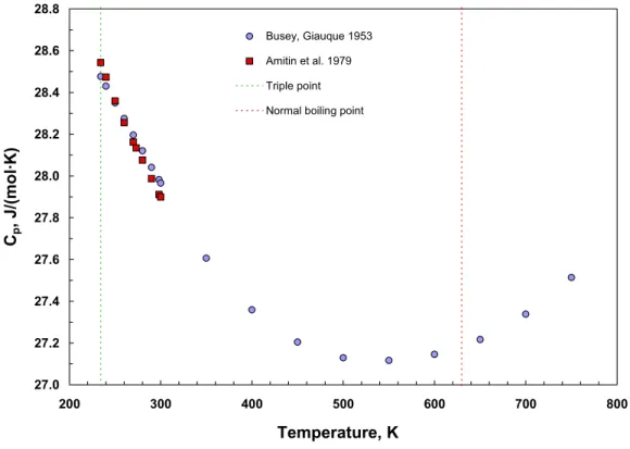
Busey and Giauque [44] measured the heat capacity Cp of mercury from 15 to 330 K with estimated uncertainties of 0.1 %. Amitin et al. [123] also measured the heat capacity mercury at temperatures from 5 K to 300 K, with an estimated uncertainty of 1 %. The smoothed data over the temperature range 234 K to 270 K from these two sources were identified as primary data for use in the regression, in addition to the primary vapor pressure data discussed

Appendix B.

For our analysis of both psat and Cp experimental data, all temperatures were first converted to the ITS-90 scale. Data taken prior to 1927 were converted to ITS-90 assuming

(16)

that the older data were on the International Temperature Scale of 1927, although we realize this introduces additional uncertainties. Except for the data of Menzies [40], all primary data were measured after 1927. The temperatures of the data of Menzies were first converted to the 1948 temperature scale by use of the procedure given by Douglas et al. [51] and then

iple t

e

t the

g the

tive

its were considered outliers and were not included in the statistics and final were converted to ITS-90.

We regressed the primary data set to three different Wagner-type expressions: the 3- 6, the 2.5-5, and a variable exponent expression where the exponents were selected from a bank of terms by use of a simulated annealing procedure [124, 125]. Simulated annealing is an optimization technique that can be used in complex problems where there may be mult local minima. It is a combinatorial method that does not require derivatives and does no depend upon “traveling downhill”; it also is relatively easy to implement. An example program using the simulated annealing to solve the Traveling Salesman Problem is given in the book by Press et al. [125]. In this work, the search space contained a bank of terms where the bank contained exponents with powers of τ in increments of 0.5, with terms up to τ¹². W followed the recommendation of Harvey and Lemmon [116] and required the equation to contain terms of order 1, 1.89, and 2, based on theoretical considerations on the behavior near the critical point. The simulated annealing algorithm was used to determine the optimal terms from the bank of terms. We implemented a Lundy and Mees [126] annealing schedule, similar to that of earlier work [127]. During the regression, one can treat the critical pressure as a variable to be determined in the regression, or it can be fixed. Due to concerns abou quality and amount of experimental data in the temperature range 930 K to 1764 K, we adopted the critical point of Kozhevnikov et al. [105] rather than determining it by fitting experimental data. The minimization was done with orthogonal distance regression usin NIST statistical package ODRPACK [128]. For the regression, the data were weighted according to their estimated uncertainty (u) with weights of 1/u². In addition, the vapor pressure data were given a relative weight factor of one, and the heat capacity data a rela weight factor of 0.02. Points that deviated by more than three standard deviations from preliminary f

regression.

The 2.5-5 form of the Wagner equation provided a better fit of the primary data set than the 3.0-6 form; further improvement resulted from the use of the simulated annealing

(17)

algorithm. Upon closer inspection, we noted that although one could reasonably reproduce the numerical value of the heat capacity, it was not possible to reproduce well the slope o the saturated liquid heat capacity near the triple point without degrading the fit in other regions. We note that the liquid heat capacity at saturation of mercury as a function of temperature displays an interesting behavior—a distinct minimum in the curve is observed below the normal boiling point, as shown in Figure 2. Douglas et al. [51] noted that other liquid metals such as sodium and potassium also exhibit this behavior. Among nonmetals, we observe that water displays this feature; however, it is not observed in simple hydrocarb such as linear alkanes. In order to simultaneously fit the vapor pressure and liquid heat capacity data, and have the correct behavior of the slope of the heat capacity as a fun temperature along the saturation boundary, we increased the number of terms in the regression

f

ons

ction of

from 5 to 6 and used the simulated annealing algorithm to obtain our final quation,

e

(

¹ ² ^1.89 ³ ² ⁴ ⁸ ⁵ ^8.5 ⁶ ⁹

)

( / _c) ( / )_c

ln p p = T T aτ +aτ +aτ +aτ +aτ +aτ . (4)

d r

21] R

= 8.314 472 J/(mol·K) and the relative atomic mass [129] of mercury, 200.59 g/mol.

The regressed coefficients and their standard deviations are given in Table 3a, and fixe parameters for eq (4) are given in Table 3b. Table 4 gives sample values of the vapo pressure calculated from eq (4) over the temperature range 273.15 to 333.15 K. For

validation of computer code, more digits than are statistically meaningful are given. For the calibration community, we also have included in Table 4 the density of saturated mercury vapor in moles per liter and nanograms per milliliter obtained assuming the ideal gas law applies, ρ = p/(R·T). We use the currently accepted values of the molar gas constant [1

(18)

27.0 27.2 27.4 27.6 27.8 28.0 28.2 28.4 28.6 28.8

200 300 400 500 600 700 800

Temperature, K Cp, J/(mol·K)

Busey, Giauque 1953 Amitin et al. 1979 Triple point Normal boiling point

Figure 2. Temperature dependence of the heat capacity of saturated liquid mercury.

(19)

Table 3a. Fitted values of the parameters in eq (4) and their standard deviations.

i ai Std. dev.

1 - 4.576 183 68 0.0472

2 -1.407 262 77 0.8448

3 2.362 635 41 0.8204

4 -31.088 998 5 1.3439

5 58.018 395 9 2.4999

6 -27.630 454 6 1.1798

Table 3b. Fixed parameters in eq (4).

Tc (K) pc (MPa)

1764 167

(20)

Table 4. Vapor pressure of mercury calculated with eq (4) from 273 K to 333 K. T, K t, °Cp, MPa Ideal gas density,† mol/L Ideal gas density,† ng/mLT, K t, °Cp, MPa Ideal gas density,† mol/L

Ideal gas density,† ng/mL 273.1502.698829·10-8 1.188337·10-8 2.383684304.15314.259045·10-7 1.684185·10-7 33.78306 274.1512.979392·10-8 1.307088·10-8 2.621887305.15324.611495·10-7 1.817581·10-7 36.45885 275.1523.286720·10-8 1.436675·10-8 2.881826306.15334.990473·10-7 1.960527·10-7 39.32620 276.1533.623129·10-8 1.577990·10-8 3.165289307.15345.397770·10-7 2.113631·10-7 42.39732 277.1543.991118·10-8 1.731989·10-8 3.474196308.15355.835283·10-7 2.277535·10-7 45.68508 278.1554.393376·10-8 1.899698·10-8 3.810605309.15366.305024·10-7 2.452917·10-7 49.20305 279.1564.832795·10-8 2.082217·10-8 4.176720310.15376.809117·10-7 2.640489·10-7 52.96556 280.1575.312487·10-8 2.280723·10-8 4.574903311.15387.349813·10-7 2.841004·10-7 56.98770 281.1585.835798·10-8 2.496477·10-8 5.007682312.15397.929493·10-7 3.055255·10-7 61.28535 282.1596.406319·10-8 2.730825·10-8 5.477762313.15408.550671·10-7 3.284075·10-7 65.87527 283.15107.027907·10-8 2.985209·10-8 5.988031314.15419.216005·10-7 3.528344·10-7 70.77506 284.15117.704698·10-8 3.261169·10-8 6.541579315.15429.928302·10-7 3.788986·10-7 76.00327 285.15128.441128·10-8 3.560348·10-8 7.141702316.15431.069052·10-6 4.066972·10-7 81.57939 286.15139.241950·10-8 3.884501·10-8 7.791920317.15441.150580·10-6 4.363324·10-7 87.52391 287.15141.011225·10-7 4.235498·10-8 8.495986318.15451.237743·10-6 4.679116·10-7 93.85838 288.15151.105749·10-7 4.615334·10-8 9.257899319.15461.330888·10-6 5.015475·10-7 100.6054 289.15161.208348·10-7 5.026135·10-8 10.08192320.15471.430383·10-6 5.373585·10-7 107.7888 290.15171.319646·10-7 5.470161·10-8 10.97260321.15481.536613·10-6 5.754690·10-7 115.4333 291.15181.440308·10-7 5.949822·10-8 11.93475322.15491.649985·10-6 6.160093·10-7 123.5653 292.15191.571046·10-7 6.467678·10-8 12.97352323.15501.770928·10-6 6.591162·10-7 132.2121 293.15201.712619·10-7 7.026452·10-8 14.09436324.15511.899890·10-6 7.049329·10-7 141.4025 294.15211.865835·10-7 7.629036·10-8 15.30308325.15522.037347·10-6 7.536097·10-7 151.1666 295.15222.031558·10-7 8.278502·10-8 16.60585326.15532.183795·10-6 8.053040·10-7 161.5359 296.15232.210708·10-7 8.978112·10-8 18.00919327.15542.339760·10-6 8.601806·10-7 172.5436 297.15242.404265·10-7 9.731323·10-8 19.52006328.15552.505789·10-6 9.184118·10-7 184.2242 298.15252.613271·10-7 1.054180·10-7 21.14581329.15562.682462·10-6 9.801783·10-7 196.6140 299.15262.838837·10-7 1.141344·10-7 22.89423330.15572.870385·10-6 1.045669·10-6 209.7507 300.15273.082141·10-7 1.235036·10-7 24.77358331.15583.070193·10-6 1.115081·10-6 223.6740 301.15283.344440·10-7 1.335691·10-7 26.79262332.15593.282555·10-6 1.188620·10-6 238.4253 302.15293.627066·10-7 1.443770·10-7 28.96059333.15603.508170·10-6 1.266503·10-6 254.0478 303.15303.931433·10-7 1.559763·10-7 31.28729 † Assumes ideal gas law applies. 17

(21)

4. Comparison with Experimental Data

For the 294 vapor pressure points in the primary data set, the average absolute deviation is 0.14 %, the bias is −0.028 %, and the root mean square deviation is 0.35 % where we use the definitions AAD = (100/n)Σabs(picalc/ piexpt − 1), BIAS = (100/n)

Σ(picalc/ piexpt − 1), and RMS² = (100/n)( Σ(picalc/ piexpt − 1)² − ((100/n) Σ(picalc/ piexpt − 1))², where n is the number of points. The AAD and RMS for the primary data are given in Table 5. The normal boiling point calculated by this equation is 629.7705 K.

Figure 3 compares the primary data set with our correlation, eq (4). The data of Ernsberger and Pitman [54] display substantial scatter, but the results are within their estimated experimental uncertainty of 1 %. The data of Shpil’rain and Nikanorov [86]

also display a fairly high scatter, but again it is within their uncertainty estimate (0.6 % to 0.8 %). The very accurate measurements of Beattie et al. [28] are in the vicinity of the normal boiling point, and the correlation, eq (4), indicates an uncertainty of 0.02 %, at a coverage factor of 2. The measurements of Spedding and Dye [87] and those of Ambrose and Sprake [18] also are represented well by our correlation, although the lowest

temperature points display larger scatter than at higher temperatures. The measurements of Menzies [39, 40] are also represented to within their estimated uncertainty. The

highest temperature data of Schönherr and Hensel [84] are represented with an AAD of 1

% and a standard deviation of 1.4 %; several points are outside of the range of the plot and are not shown. The correlation is valid to the critical point at 1764 K, but does not account for a metal-nonmetal transition [63] in mercury at approximately 1360 K that results in a change of slope in the vapor pressure curve.

(22)

Table 5. Summary of comparisons of the correlation with the primary data for the vapor pressure of mercury.

First author No.

pts.

T range, K

Estimated uncertainty, % AAD

%

RMS

%

Ambrose [18] 113* 417-771 less than 0.03, greatest at lowest T 0.02 0.06

Beattie [28] 42 623-636 0.03 0.01 0.01

Ernsberger [54] 18 285-327 1 0.33 0.35

Menzies [39, 40] 46** 395-708 0.5 0.14 0.20

Schönherr [84] 13 1052- 1735

3 1.06 1.42

Shpil’rain [86] 50 554-883 0.6-0.8 0.25 0.29

Spedding [87] 13 534-630 0.03 0.05 0.06

* Two outliers at 380 K and 400 K were not included in statistics.

** One outlier at 395 K was not included in statistics.

-1 -0.8 -0.6 -0.4 -0.2 0 0.2 0.4 0.6 0.8 1

200 700 1200 1700

Temperature, K 100·[(p-peq(4))/p]

Ambrose, Sprake 1972 Spedding, Dye 1955 Shpil'rain, Nikanorov 1971 Menzies 1910,1927 Beattie et al. 1937 Ernsberger, Pitman 1955 Schönherr, Hensel 1981

Figure 3. Deviations between the correlation given in eq (4) and the primary data set.

(23)

Figure 4 compares selected data not used in the regression (secondary data) with the correlation eq (4), and Table 6 summarizes comparisons with all secondary data. It is interesting to note that the behavior of the correlation at low temperatures falls in

between the values of Douglas et al. [51] and those of Busey and Giauque [44]. Both of these sets were not obtained from direct vapor pressure measurements, but rather were calculated based upon caloric measurements combined with vapor pressure data at higher temperatures. The data of Schmahl et al. [82] cover a range of temperature from 412 to 640 K and are in good agreement with the correlation. The measurements of Burlingame [43] and of Dauphinee [49,50] were made by use of a transpiration technique with uncertainties on the order of 4 to 5 %, and the correlation represents them within this range of deviations. Figure 4 also displays considerably more scatter at both the high and low temperature ends of the plot.

-10 -8 -6 -4 -2 0 2 4 6 8 10

200 400 600 800 1000

Temperature, K 100·[(p-peq(4))/p]

Douglas et al. 1951 Burlingame 1968 Busey, Giauque 1953 Dauphinee 1951 Murgulescu, Topor 1966 Schmahl et al. 1965 Sugawara et al. 1962 Volmer, Kirchoff 1925 Roeder, Morawietz 1956 Hildenbrand et al. 1964 Cailletet et al. 1897 Rodebush, Dixon 1925

Egerton 1917 Poindexter 1925

Figure 4. Deviations between the correlation given in eq (4) and selected secondary data.

(24)

Table 6. Summary of comparisons of the correlation given in eq (4) with secondary data for the vapor pressure of mercury.

First author No. pts. T range, K

Estimated uncertainty,

%

AAD % RMS % Bernhardt [41] 27 694-1706 varies from 2 to >15 14.13 17.26 Bessel-Hagen [42] 2 273-293 >20 96.12 2.50

Burlingame [43] 38 344-409 4 1.44 1.92

Busey [44] 24 234-750 varies from 0.2 to 3.5 at lowest T 0.90 1.03 Cailletet [45] 11 673-1154 varies from 1 to7 3.97 2.26

Callendar [46] 2 630 0.2 0.17 0.14

Cammenga [47] graphical results 273-325

Carlson [48] 9 299-549 varies from 3 to >20 19.74 16.83

Dauphinee [49, 50] 18 305-455 5 2.14 2.94

Douglas [51] 30 234-773 var. from 0.03 (at normal boiling

point) to 1.5 at lowest T 0.45 0.54

Durrans [52] 19 290-344 4.63 3.06

Egerton [53] 27* 289-309 5 6.99 2.34

Galchenko [55] graphical results 523-723 3 na na

Gebhardt [57] 9 403-483 8 3.34 4.03

Haber [37] 1 293 2 1.84 na

Hagen [58] 5 273-473 >20 51.02 57.44

Hensel [59] graphical results 1073-critical na na na

Hertz [35] 9 363-480 5 4.50 1.94

Heycock [60] 1 630 0.2 0.21 Na

Hildenbrand [61] 6 295-332 5 2.76 3.16

Hill [62] 19 272-308 30 29.40 4.38

Hubbard [63] graphical results 742-1271 na na na Jenkins [64] 21 479-671 varies from 0.1 to >20 5.08 5.67

Kahlbaum [65] 43 393-493 >10 8.89 9.47

Knudsen [66] 10 273-324 varies from 5 to 10 7.36 1.67 Knudsen [67] 7 263-298 varies from 5 to 10 7.12 7.64

Kordes [68] 2 630-632 4 2.59 1.84

Mayer [69] 82 261-298 5, except greater at T<270 6.72 8.86

McLeod [70] 1 293 >20 77.65 na

Millar [71] 6 468-614 2 1.27 1.84

Morley [72] 6 289-343 varies from 8 to >20 17.58 11.82

Murgulescu [73] 9 301-549 3 1.41 1.56

Neumann [74] 19 290-344 6 4.63 3.06

Pedder [75] 3 559-573 2 1.14 0.94

Pfaundler [76] 3 288-372 12 8.06 5.76

Poindexter [77] 17 235-293 >5-20; greatest at lowest T 28.23 29.19 Ramsay [36] 13 495-721 varies from 0.3 to 10 at highest T 3.23 3.02 Regnault [33] 29 297-785 ~6 for T>400, much higher for