Fitting simulated random events to experimental histograms by means of parametric models

Fitting simulated random events to experimental histograms by means of parametric models

Oliver Kortner

^a,

*, Cˇrtomir Zupan W i W

^b

aMax-Planck-Institut fur Physik, F. ohringer Ring 6, D-80805 M. unchen, Germany.

bLudwig-Maximilians-Universitat M. unchen, Am Coulombwall 1, D-85748 Garching, Germany.

Received 12 April 2001; received in revised form 13 January 2003; accepted 17 February 2003

Abstract

Classical chi-square quantities are appropriate tools for fitting analytical parameter-dependent models to (multidimensional) measured histograms. In contrast, this article proposes a family of special chi-squares suitable for fits with models which simulate experimental data by Monte Carlo methods, thus introducing additional randomness. We investigate the dependence of such chi-squares on the number of experimental and simulated events in each bin, and on the theoretical parameter-dependent weight linking the two kinds of events. We identify the unknown probability distributions of the weights and their inter-bin correlations as the main obstacle to a general performance analysis of the proposed chi-square quantities.

r

2003 Elsevier Science B.V. All rights reserved.

PACS: 02.50.Ph; 02.50.Sk; 07.05.Kf

Keywords: Chi-squares; Variances of simulated histograms; Maximum likelihood

1. Introduction

1.1. Need for chi-squares in particle physics A typical experimental apparatus in particle physics detects events (statisticians would call them

‘‘elementary’’). In each event, either an ‘‘initial’’

(incoming) particle decays into several ‘‘final’’

(outgoing) particles or two initial particles collide

to produce the final particles. Ideally, the 3- momenta and spin directions of the initial particles are selected and those of the final particles are measured by the apparatus. Events may thus be represented by points in the (generally multi- dimensional) phase space [1–4], formed by the 3- momentum components and helicities of the final particles. We assume that the phase space has been reduced to its relevant coordinates by eliminating those on which, for symmetry reasons, the differential cross section or decay probability cannot depend. A simple example of the latter coordinates are the spin directions in case of unpolarized initial particles and of undetected helicities of the final particles.

*Corresponding author. Tel.: +4989-32354240; fax: +4989- 3226704.

E-mail address: oliver.kortner@cern.ch, kortner@mpp- mu.mpg.de (O. Kortner).

0168-9002/03/$ - see front matterr2003 Elsevier Science B.V. All rights reserved.

doi:10.1016/S0168-9002(03)00985-9

Theory may predict the result of the measure- ment, i.e. the differential cross section or decay probability but, in most interesting cases, the theoretical model contains parameters to be determined (statisticians say: estimated) from the comparison between experimental data and model predictions. The latter have to take into account the experimental conditions, in particular the imperfect resolution and acceptance of the appa- ratus. Nowadays, with ever more complex appa- ratus and ever more powerful computers, the final predictions of the model are most often obtained by Monte Carlo (MC) simulations. The compar- ison between model and experiment then requires a fit of the model density to the experimental density. Both consist of points in phase space but the simulated points are provided with parameter dependent weights from the theoretical model. The optimal values of the parameters are obtained by minimizing suitable random functions of the parameters such as different chi-square quantities or negative logarithms of maximum likelihood;

(statisticians call this procedure point estimation).

A standard computer program for this purpose is MINUIT [5] which also explores the form of the many-dimensional parameter valley in the vicinity of the optimal value of the parameter vector (interval estimation).

The principal motivation for this article stems from meson spectroscopy where the number of measured events from a single final channel may nowadays reach the order of magnitude of 10

⁶

; only to be matched by a comparable or even larger number of simulated events (see, e.g. Ref. [6]).

However, often the dimension of the reduced phase space is also high and the experimental resolution quite good, so that the phase space density of events (defined as the number of events in the smallest experimentally identifiable element of phase space) may still be very low.

At such low densities, maximum likelihood estimation using individual (unbinned) events is the method of choice. Unfortunately, it has at least three disadvantages:

(1) It is not easily combined with a reliable correction for imperfect 3-momentum resolu- tion of the apparatus.

(2) It does not by itself furnish a quantitative measure of goodness-of-fit [7].

(3) On a present-day desk-top computer it is prohibitively time and memory consuming, if the number of events and their complexity are as high as or even higher than in reference [6].

1.2. Binning and the classical Neyman chi-square In order to avoid these disadvantages, one is tempted to sacrifice some of the information contained in the experimental data by grouping events into bins. Then the fit may be performed by minimizing a suitable chi-square quantity X

²

: (Here, X should be read as a capital w and not as a capital x: We follow the modern trend of the statistical literature in reserving the symbol w

²

for the w

²

probability distribution.) A X

²

quantity is defined as

X

²

¼ X

i

X

_i²

ði ¼ 1; 2; y ; KÞ: ð1Þ The summation in Eq. (1) runs over all bins i ¼ 1; 2; y ; K where K is the total number of bins.

Here and later this should be understood whenever we use the symbol P

i

: When introducing a new X

²

we shall mostly not explicitly repeat the standard equation (1). The characterizing index of X

_i²

(e.g. X

_N;i²

for the Neyman X

_i²

; see below) should be understood to symbolize the corre- sponding total X

²

quantity as well (e.g. X

_N²

). The contribution X

_i²

of bin i to X

²

may, for instance, have the form

X

_i²

¼ ðy

_i

n

i

Þ

²

s

²_i

ð2Þ

where n

_i

is the number of experimental events in bin i; y

_i

is the model prediction for n

_i

; and s

²_i

is some measure of the variance of y

_i

n

_i

:

Typically, the number of bins K is chosen so large that the total number of experimental events N ¼ X

i

n

_i

ð3Þ

is much larger than any individual bin content n

_i

:

Then we may safely assume that n

i

is a Poisson

distributed random variable. Of course, y

i

depends

on the parameter vector ~ y y ¼ ðy

₁

; y

₂

; y ; y

r

Þ where r is the number of parameters but, as a rule, y

i

is assumed not to explicitly depend on any random variable. Under this condition, we may convert expression (2) into the classical Neyman

1

X

_N;i²

(also called ‘‘modified’’ X

_i²

) by setting

s

²_i

¼ n

i

ð4Þ

which leads to

1

X

_N;i²

¼ ðy

_i

n

i

Þ

²

n

_i

: ð5Þ

1

X

_N²

is antedated by the classical Pearson

₁

X

_P²

; cf. Section 2; for the terminology, see e.g. Refs.

[8–10].

The lower index 1 on the left of the symbol X

_N;i²

in Eq. (5) indicates that this quantity which we call univariate depends on a single random variable n

_i

: The entire set of bin contents n

_i

may be considered as a single random vector ~ n n in a K-dimensional space

~ n

n ¼ fn

_i

; i ¼ 1; 2; y ; Kg ð6Þ so that referring to any

₁

X

²

¼ P

i1

X

_i²

as a univariate chi-square quantity is also justified.

(Analogously we may define other K-dimensional vectors, e.g. ~ y y:)

1.3. Weights of events generated by Monte Carlo On the other hand, if y

i

has been obtained by a MC simulation, it does depend on the random number m

i

of simulated events in bin i: Then we replace y

i

ð ~ y y Þ by f

i

ð ~ y yÞm

_i

where f

i

ð ~ y yÞ is a ~ y y-dependent weight obtained as the average of the theoretical weights f

_ij

ð ~ y yÞ of individual MC events in bin i; i.e.

f

i

ð ~ y yÞ ¼ 1 m

_i

X

^mi

j¼1

f

ij

ð ~ y yÞ ðj ¼ 1; 2; y ; m

i

Þ: ð7Þ For typographic reasons we prefer the symbol f to the more common one w for ‘‘weight’’. Below we often simplify the notation by writing f

ij

instead of f

ij

ð ~ y yÞ and f

i

instead of f

i

ð ~ y yÞ: In complete analogy with Eq. (3), we define the total number of simulated events M by

M ¼ X

i

m

_i

: ð8Þ

The individual weights f

ij

depend on the method chosen to generate the MC events. Often they are generated by the GENBOD program [2] which also yields the corresponding weight f

_ij^ðGÞ

propor- tional to the phase space element [1] in the GENBOD set of coordinates; the proportionality constant, common to all bins, depends on global quantities such as M; N; the experimental lumin- osity, etc. The weight f

_ij^ðGÞ

may be multiplied by the norm jTj

²

of the theoretical transition (i.e. reaction or decay) amplitude at the phase space point of the generated event, resulting in the final weight f

_ij

: Alternatively, f

_ij^ðGÞ

may be used by the hit-or-miss stratagem (also called acceptance–rejection meth- od [11]) to generate events distributed with phase space density; in that case f

ij

is proportional to jT j

²

:

1.4. Reconstruction of Monte Carlo events

We refer to the coordinates and the density adopted for the generation of the simulated events as the ‘‘MC generation space’’. Note that Eq. (7) does not imply a simple summation; in general, the summation is preceded by a tedious tracking and reconstruction needed to find the bin (or the garbage can) in which the generated event ends after all distortions have been taken into account.

Therefore, the ‘‘MC reconstruction space’’ is not equal to the MC generation space, in general. Only the MC reconstruction space has to be binned and used to class the experimental events as well. Note also that, in practice, the sizes and shapes of the bins depend on the choice of the phase space coordinates.

1.5. The randomness of weights

In general, not only m

_i

but also f

_i

is a random

quantity: for finite values of m

_i

it becomes a matter

of chance how many simulated events fall into

regions of small and how many into regions of

large theoretical differential cross section (or decay

probability) in bin i . If m

_i

; n

_i

; and f

_i

are mutually

uncorrelated (see Sections 2 and 6), a simple

estimate of the variance Varð f

i

m

i

n

i

Þ is provided

by the standard rules of error propagation in

the form

s

²_i

¼ f

_i²

Varðm

_i

Þ þ m

²_i

Varð f

i

Þ þ Varðn

_i

Þ

¼ ð f

_i²

þ M

_2;i

Þm

_i

þ n

_i

ð9Þ with

Varð f

_i

Þ ¼ 1

m

_i

M

_2;i

¼ 1 m

_i

ðm

_i

1Þ

X

^mi

j¼1

ð f

_ij

f

_i

Þ

²

" # :

ð10Þ Of course, this estimate is possible only under the condition m

i

X 2: Remember that Varð f

i

Þ and M

2;i

are functions of ~ y y: Note that M

2;i

is an unbiased estimator of the variance of the probability distribution of the weights f

ij

in bin i: In Section 6 we shall define this variance as the second central moment M

2;i

(cf. Eq. (87)).

1.6. The case m

i

p1

If m

_i

p 1; Eq. (10) cannot be used, and for m

_i

¼ 0 also Eq. (7) is meaningless. In both cases a straightforward remedy is to increase M or decrease K (or both). However, if none of these solutions is acceptable, an approximate one might be offered by generating additional events only in bins which are likely to contribute to bin i; and to evaluate f

i

with those among them which end up in bin i after reconstruction. However, they should not be added to the total sample of M originally simulated events, or else the probability distribu- tion of m

i

would be modified in a way difficult to control. Obviously, this prescription is applicable only to cases when only a few out of the total number of K bins contain no simulated events and when the experimental resolution is good enough so that any bin with m

_i

¼ 0 requires additional generation only in a small portion of the available MC generation space.

1.7. Nonrandom weights and the bivariate Neyman chi-square

For most of the present article, i.e. until its Section 6, we assume

M

2;i

5 f

_i²

: ð11Þ

The main reason for this preliminary assumption are the unknown probability distributions of the random weights f

ij

: They depend on the particular theoretical model describing a specific experiment, as well as on the boundaries of the bins, thereby precluding as detailed investigations of different chi-square quantities as are feasible if the random nature of the weights f

i

may be neglected.

Under the assumption (11), Eq. (9) reduces to s

²_i

¼ f

_i²

m

_i

þ n

_i

: ð12Þ We define

2

X

_N;i²

¼ ð f

_i

m

_i

n

_i

Þ

²

f

_i²

m

_i

þ n

_i

ð13Þ

which depends on two random quantities m

_i

and n

_i

: We refer to such

₂

X

_i²

and to the corresponding

2

X

²

quantities as bivariate and label them by a lower left index 2. The subscript N reminds us that expression (13) is an adaptation of the classical univariate Neyman

1

X

_N;i²

; designed to take into account the statistical uncertainties of both the experiment and the simulation (provided assump- tion (11) is valid). A more convincing justification of Eq. (13) is to be found in Section 2 and Appendix B.

1.8. The classical Baker–Cousins chi-square Nearly two decades ago, Baker and Cousins [9]

have advocated the use of chi-square quantities obtained from ratios of likelihoods. (Note that their symbol m m ~ has a different meaning from ours.) Specifically, for Poisson-distributed binned data they highlight

1

X

_l²

¼ X

i

1

X

_l;i²

ð14Þ

with

1

X

_l;i²

¼ 2½y

_i

n

i

þ n

i

lnðn

_i

=y

i

Þ ð15Þ as a convenient chi-square quantity for point estimation, interval estimation, and goodness-of- fit testing. (In Ref. [9]

₁

X

_l²

is denoted by w

²_l;p

; p stands for Poisson.) Contrary to the classical Neyman

₁

X

_N;i²

of Eq. (5), expression (15) remains finite even if n

i

¼ 0; and it is easy to ensure that

1

X

_l²

‘‘preserves the area’’, i.e., that the fitted total

number of events equals their measured number.

The Particle Data Group has been independently recommending

1

X

_l²

in the prestigious Review of Particle Physics, starting with its 1988 issue [12].

However,

1

X

_l²

as defined above behaves as a classical likelihood-ratio chi-square only for nonrandom y

i

: Therefore, it is not optimally suited for the case of greatest interest in modern particle physics, that of theoretical predictions obtained by MC simulations.

1.9. Related work

The problem of fitting experimental histograms by randomly simulated model histograms has been previously discussed by Schmidt et al. [13] from a more practical standpoint than ours, but without taking into account the statistical uncertainties of the simulation in the fitting algorithm itself. We recommend their paper and, of course, that of Baker and Cousins as an additional introduction to the present article. A more sophisticated method than ours to take into account the random nature of theoretical predictions in the fitting algorithm has been proposed by Eberhard et al.

[14] for the special case of an adjustable linear superposition of several model distributions, each of them produced by a parameter-free MC simulation. An informative and original but quite condensed review article on the subject by Zech [15] has unfortunately remained unpublished. It reviews also unfolding, i.e. the experimentalist’s attempt to correct the measured data for imperfect acceptance and resolution of the apparatus before presenting them to the theorist (see also Ref. [16]).

We assume throughout our article that it is the job of the theorist to take experimental imperfections into account in the simulation—a less desirable (especially from the theorist’s point of view) but often unavoidable alternative to unfolding.

1.10. Preview of the present article

The purpose of the present article is to introduce a special family of bivariate chi-square quantities which take into account the random nature of both the experimental data and their theoretical simulations. They are asymptotically equivalent and w

²

distributed. They differ at finite values of m

i

and n

i

but they all remain finite when any of these bin contents vanish. We consider in more detail a few special chi-squares which exhibit scaling properties making their presentation relatively simple, and we discuss their characteristics at small values of m

i

and n

i

: In a subsequent article II [17] we shall try to correlate these characteristics with the suitability of the corresponding chi- square quantities for goodness-of-fit tests and with their performance in fitting the area of the histogram. At the end of the present article we convert the bivariate chi-square quantities into trivariate ones by multiplying them with simple bin-dependent correction factors which take in a primitive way into account the statistical fluctua- tions of the weights f

i

:

2. More on the bivariate Neyman chi-square 2.1. Statistical independence of bin contents

In the preceding section we have tacitly assumed that the K K covariance matrix S [18] is diagonal with the elements s

²_i

: This is certainly true before the fit, provided the systematic errors are negligible and provided the boundaries of the bins are chosen without regard to the results of either the experiment or the simulation. Then the bin contents n

_i

are statistically independent of the bin contents m

_j

and the weights f

_j

ð ~ y y Þ; for any possible values of i and j: Any triplet m

i

; n

i

; f

i

ð ~ y yÞ is statistically independent of another triplet m

j

; n

j

; f

j

ð ~ y yÞ with iaj: The weight f

i

ð ~ y yÞ is not independent of m

i

; as is evident from Eq. (7). However, m

i

and f

i

ð ~ y yÞ are not correlated, since the latter is an unbiased estimate of the expectation value of f

i

ð ~ y yÞ for any value of ~ y y that leads to real nonnegative weights f

ij

ð ~ y yÞ; and for any integer value of m

i

> 0;

see the next subsection for a justification of this statement and Section 1.6 for a possible treatment of the case m

_i

¼ 0: Further comments on systema- tic errors are deferred to Section 2.3.

2.2. Expectation values and ‘‘true’’ values of random quantities

In statistics it is customary to contemplate a

countably infinite set O of statistically independent

but otherwise equal experiments and simulations.

In simple cases, it is feasible but time-consuming to realize an approximation to O by a set O

fin

with a finite but preferably large number N

O

of elements.

In the set O; the content m

i

or n

i

of a given bin i is an ‘‘independent identically distributed (i.i.d.)’’

random variable. With respect to this set we define the expectation values

m

_i

Eðm

_i

Þ ¼

^def

lim

N_O-N

1 N

_O

X

^NO

1

m

i

;

n

_i

Eðn

_i

Þ ¼

^def

lim

N_O-N

1 N

O

X

^NO

1

n

_i

: ð16Þ

Note that in Eqs. (16) the summations extend over the elements of the set O

_fin

and not over the bins i:

Henceforth, the symbol E will always indicate an expectation value with respect to the set O:

We assume the distributions of m

_i

and n

_i

to be Poisson, i.e. of the form

Pðm

_i

jm

_i

Þ ¼ e

^mi

m

^m_iⁱ

m

_i

! ; Pðn

_i

jn

_i

Þ ¼ e

ⁿⁱ

n

ⁿ_iⁱ

n

_i

! : ð17Þ The expectation values m

_i

and n

i

are positive nonrandom and, in general, nonvanishing real numbers. (If the theory is sensible and the simulation correct, m

_i

and n

_i

for a given bin i can vanish only together and only if the experimental acceptance vanishes for bin i: In this case, bin i may simply be omitted from further considera- tion.) Because the set O is approximately realiz- able, both m

_i

and n

i

—though rarely known in practice—are physically measurable quantities, in principle. If systematic errors in the counting of events and assigning them to the particular bin i are avoided or corrected for, m

_i

and n

i

may as well be called the true values of m

i

and n

i

; respectively.

Similarly to m

_i

and n

i

; we can define the expectation values / f

_i

S E½f

_i

ð ~ y yÞ which are non- random positive functions of ~ y y: However, we shall have little use for these quantities except to justify the statement in the preceding subsection about the absence of a correlation between m

_i

and f

_i

: Assume that in a particular element of the set O the value of m

_i

is larger than m

_i

; since f

_i

ð ~ y yÞ of Eq. (7) is an unbiased estimator of / f

_i

S ; it is on the average equally probable that the correspond- ing value of f

i

/ f

i

S is positive or negative, i.e.

E½ð f

i

/ f

i

S Þðm

i

m

_i

Þ ¼ 0 which means that m

i

and f

i

are not correlated. As an illustration, consider f

i

¼ P

mi

j¼1

f

ij

=ðm

_i

þ xÞ with x being any positive real number. This f

i

is a consistent but biased estimator of the expectation value / f

i

S ; it is positively correlated with m

i

for nonvanishing values of x: Incidentally, as suggested in Section 1.6, it is perfectly possible (only time-consuming) to find f

i

independently of the MC simulation serving to fit the experimental data, thus making f

_i

totally independent of m

_i

:

Provided m

_i

a 0; we can define the true values f

_i

of f

_i

by

f

_i^def

¼ n

i

m

_i

: ð18Þ

They are also positive real numbers but they do not depend on ~ y y: (In the genuinely bivariate case of model predictions obtained by MC simulations, f

_i

could vanish only in case of a wrong simulation yielding m

_i

> 0 in spite of n

i

¼ 0 — or diverge if the wrong simulation yields m

_i

¼ 0 in spite of n

i

> 0: As for the univariate limit f

_i

-0; m

_i

- N with finite n

_i

¼ f

_i

m

_i

; see Appendix A.) Note, though, that f

_i

cannot be defined as Eðn

_i

=m

_i

Þ: The latter expecta- tion value does not even exist, since m

_i

¼ 0 is among the possible values of the random variable m

_i

: Therefore, the alternative naming of f

_i

as the

‘‘true value of the ratio q

_i

¼ n

_i

=m

_i

’’ could be misleading.

2.3. The ‘‘true’’ value of the parameter vector ~ y y The operational definition of the true value ~ y y

t

of the vector ~ y y is not as simple. The latter cannot be measured directly but it is obtained as the result of the fit. Assume that we know the correct theory (up to the value of ~ y y), that we have perfect information on the performance of the experi- mental apparatus, and that the systematic errors are known to be negligible as compared to statistical ones. Nevertheless, the estimates of ~ y y will most often be biased and bias cannot be reduced by independent repetitions of experiment, simulation, and fit, i.e. by building up the set O:

The solution—provided the estimate of ~ y y is

consistent—is to aim at the asymptotic limit

m

_i

- N ; n

i

- N ; with n

i

=m

_i

¼ f

_i

¼ const:a0 for

all i ¼ 1; 2; y ; K (see the next subsection). The results are increasingly accurate statistics ~ y y ; i.e.

vector functions of the (increasingly large) bin contents m

i

and n

i

: In this sense, even ~ y y

t

may be considered as a physically measurable quantity.

Henceforth, whenever we use the symbol ~ y y

t

; we imply that the above assumptions are valid.

Hence, our implicit definition (under the above provisos) of ~ y y

t

is

m_i-N;f

lim

_i¼const:a0

E½f

_i

ð ~ y y

t

Þ ¼ f

_i

ð19Þ (see also Section 6).

Unfortunately, our model is often based on a theory which is only partially known and calcul- able (e.g. QCD which is reliably calculable only in the perturbative region). At best, the consequences of the unknown part can be crudely estimated as a so-called systematic theoretical error. Actually, since we have assumed (cf. Section 1.9) that imperfections of the experimental apparatus are to be faithfully simulated by the theorist, any errors in this simulation might as well be termed

‘‘theoretical’’ or—better—we should call any nonstatistical and uncorrectable error simply

‘‘systematic’’. As a rule, systematic errors cannot be reduced by identically repeating the experiment and its analysis. Therefore they furnish an irreducible limit to the measurability of ~ y y

_t

: In addition, systematic errors generally cause correla- tions between weights of different bins and—if they are important—nondiagonal covariance ma- trices S should enter our chi-squares. We shall not attempt a corresponding extension of the present article, though we are conscious that its scope is therefore severely limited.

2.4. Ideal form

2

X

²_N;i

of

2

X

_N;i²

and its asymptotic limit

2

X

²_N;i

The quantity

2

X

_N;i²

of Eq. (13) with f

i

substituted by f

_i

; i.e.

2

X

²_N;i

¼ ðf

_i

m

_i

n

_i

Þ

²

f

²_i

m

i

þ n

i

ð20Þ is, in a sense, the ‘‘ideal’’ value of

₂

X

_N;i²

; given a pair of event numbers m

i

and n

i

; it is neither the expectation nor the true value of

2

X

_N;i²

: Hence-

forth, the qualifier ‘‘ideal’’ should be considered a technical term and we omit the quotation marks.

The quantity

2

X

²_N;i

does not depend on the parameter vector ~ y y and cannot be used for point or interval estimation but it is of theoretical interest.

Here, we consider the limiting value of

₂

X

²_N;i

in the asymptotic case m

_i

- N ; n

_i

- N with 0 o f

_i

¼ n

_i

=m

_i

¼ const: o N : (Note that our use of the term

‘‘asymptotic’’ does not refer to the infinite number N

_O

of elements in the set O: Subsequently, we shall not always repeat the definition of this term.) We replace m

i

and n

i

by new variables d

i

and e

i

; respectively, defined by

d

i^def

¼ m

i

m

_i

; e

i^def

¼ n

i

n

i

: ð21Þ Since we have assumed that m

i

and n

i

are Poisson distributed, we have

Eðd

_i

Þ ¼ Eðe

_i

Þ ¼ 0; Eðd

²_i

Þ ¼ m

_i

; Eðe

²_i

Þ ¼ n

_i

: ð22Þ To 0th order in 1=n

i

and 1=m

_i

; i.e. if

E d

²_i

m

²_i

¼ 1

m

_i

-0; E e

²_i

n

²_i

¼ 1

n

i

-0 ð23Þ we obtain

2

X

²_N;i

-

2

X

²_N;i

ð24Þ

with

2

X

²_N;i

¼ ðf

_i

d

i

e

i

Þ

²

n

_i

ðf

_i

þ 1Þ : ð25Þ

2.5. Asymptotic w

²

ð1Þ behaviour of

2

X

²_N;i

The quantity

2

X

²_N;i

may be considered as a nonnegative random variable z

i

which depends on two parameters f

_i

and n

i

: The variable z

i

is distributed according to a distribution F ðz

_i

; f

_i

; n

i

Þ which is not explicitly known. However, in the limit n

_i

- N ; f

_i

¼ const: a 0; the distribution of z

_i

approaches the distribution of the variable z ¼ w

²

ð1Þ; irrespective of the value of f

_i

:

This statement may be justified by the following

argument. In the limit n

_i

- N ; the Poisson

distribution Pðn

_i

jn

_i

Þ approaches a Gaussian dis-

tribution Nðn

_i

; n

i

Þ (i.e. with mean n

i

and variance

n

i

) [19]. Therefore, the asymptotic distribution of

the random variable d

i

¼ f

_i

m

i

n

i

¼ f

_i

d

i

e

i

is given by the folding [20] of the Gaussian Nðf

_i

m

_i

; f

²_i

m

_i

Þ with the Gaussian Nðn

_i

; n

i

Þ: The resulting distribution is again a Gaussian with the mean f

_i

m

_i

n

i

¼ 0 and the variance f

²_i

m

_i

þ n

i

¼ n

i

ðf

_i

þ 1Þ: Therefore [19,21], the variable z

i

¼ d

_i²

=½n

_i

ðf

_i

þ 1Þ ¼

₂

X

²_N;i

is asymptotically (i.e. for m

_i

- N ; n

i

¼ f

_i

m

_i

- N ; f

_i

¼ const:Þ w

²

ð1Þ dis- tributed.

An alternative proof of the above statement, outlined in Appendix B, is based on the Second Limit Theorem [22], i.e. on the equality of the asymptotic moments of F ðz

_i

; f

_i

; n

_i

Þ with the mo- ments of w

²

ð1Þ: Appendix B also contains some information on the moments of

₂

X

²_N;i

and of similar quantities (see the next section) outside the asymptotic region, which is of interest for Section 6 and article II [17].

It is easy to see that the w

²

ð1Þ asymptotic distribution of

2

X

²_N;i

implies that

2

X

²_N;i

is asymp- totically w

²

ð1Þ distributed. Sometimes we state simply that these quantities ‘‘are asymptotically w

²

ð1Þ’’. Somewhat sloppily, one may also say that

2

X

_N;i²

itself is asymptotically w

²

ð1Þ distributed though, of course, this is not generally true if the simulation uses a poor model or if ~ y y differs substantially from ~ y y

_t

:

2.6. Self-conjugacy and regularity of

2

X

_N;i²

The quantity

2

X

_N;i²

has some additional remark- able properties. From a statistical point of view, the random number of experimental events n

i

and the random number of simulated events m

i

are equivalent. Therefore, instead of trying to find the factors f

i

which are best suited to convert—as closely as possible—m

_i

into n

_i

for all bins i; we may try to find the factors g

_i

best suited to convert n

_i

into m

_i

: The bivariate chi-square quantity suitable for that purpose may be obtained from

₂

X

_N;i²

of Eq. (13) by the simultaneous interchanges

m

_i

2 n

_i

ð26Þ

f

_i

2 g

_i

: ð27Þ

However, from the point of view of physics, the experimental and the MC events are not equiva- lent. Both the generated (i.e. actual) and the

reconstructed (i.e. apparent) coordinates in phase space are known for MC events, but only the latter are measured for experimental events. As a consequence, if the imperfect resolution of the apparatus is to be taken into account, g

i

should be taken as

g

i

¼ 1=f

i

ð28Þ

and f

_i

ð ~ y yÞ evaluated using generated and recon- structed MC events in any case. (Here we have emphasized the dependence of f

_i

on ~ y y which is at this point a parameter vector yet to be estimated later by the fit.) Therefore, Eq. (27) must be replaced by

f

i

2 1=f

i

: ð29Þ

The interchange (26) implies

m

_i

2n

i

and f

_i

21=f

_i

: ð30Þ As may be easily verified,

2

X

_N;i²

of Eq. (13) is invariant with respect to the simultaneous inter- changes (26) and (29). For m

_i

> 0 and n

_i

> 0;

₂

X

_N;i²

vanishes at

f

_i^ðextrÞ

¼ n

_i

m

i

ð31Þ in concordance with the invariance with respect to the interchanges (26) and (29).

2

X

_N;i²

stays finite for m

i

¼ 0; n

i

a0 and (therefore) for n

i

¼ 0; m

i

a0: At m

_i

¼ n

_i

¼ 0 it may be set to zero, since it is a ratio of two forms in m

_i

and n

_i

with the form in the numerator being of higher degree than the one in the denominator.

3. A family of special bivariate chi-square quantities

3.1. ‘‘Specialness’’ and conversion of a univariate

1

X

_i²

into the corresponding special bivariate

2

X

_i²

We call ‘‘special’’ (which should be considered a technical term) any bivariate

₂

X

²

quantity and its components

₂

X

_i²

; if the latter have the following properties:

(1) asymptotic w

²

ð1Þ distribution,

(2) invariance w.r.t. the simultaneous inter-

changes (26) and (29) (subsequently referred

to as the pair (26), (29)),

(3) finite values at m

i

¼ 0 and at n

i

¼ 0;

(4) minimal value zero at f

i

¼ f

_i^ðextrÞ

¼ n

i

=m

i

; if m

i

> 0 and n

i

> 0:

In addition, as announced in Section 2.3, correlations between different bins i are disre- garded in our special

2

X

²

quantities.

We have just seen that

2

X

_N²

is special. Below we introduce a family of such special bivariate chi- square quantities. Starting from familiar univari- ate

₁

X

_i²

quantities, we first replace the theoretical prediction y

_i

by f

_i

m

_i

: Then we check the asympto- tic distribution of the resulting

₂

X

_i²

and, if necessary, multiply the latter by a suitable correc- tion factor so as to achieve an asymptotic w

²

ð1Þ distribution. If this

2

X

_i²

still lacks any of the properties 2. – 4., we ‘‘specialize’’ it by taking a suitable linear superposition of

2

X

_i²

and its conjugate

2

X

_i^2;c

w.r.t. the pair (26), (29).

Conversely, starting from any given bivariate

2

X

_i²

—be it special or not—we may recover the corresponding univariate

1

X

_i²

if we replace f

i

m

i

by y

i

; set the remaining f

i

to zero, and take into account that n

_i

5 m

_i

(cf. Eqs. (5) and (13)). A mathematically more transparent and general prescription for the limiting process leading from a bivariate

₂

X

_i²

to the corresponding univariate

1

X

_i²

is to be found in Appendix A.

3.2. The special

2

X

_P;i²

and

2

X

_R;i²

It is not difficult to find a simple special

2

X

_P;i²

¼ ð f

i

m

i

n

i

Þ

²

f

_i

m

_i

ðn

_i

=m

_i

þ 1Þ ¼ ð f

i

m

i

n

i

Þ

²

f

_i

ðm

_i

þ n

_i

Þ ð32Þ which reduces in the univariate limit to the classical Pearson

1

X

_P;i²

¼ ðy

_i

n

i

Þ

²

y

_i

: ð33Þ

The ratio G

i ^{def 2}

¼ X

_P;i²

2

X

_N;i²

¼ f

_i²

m

_i

þ n

_i

f

i

ðm

_i

þ n

i

Þ ð34Þ is (necessarily) invariant w.r.t. pair (26), (29), and finite both at m

i

¼ 0; n

i

a0 and at n

i

¼ 0; m

i

a0: Its

ideal form G

i

¼ f

²_i

m

i

þ n

i

f

_i

ðm

_i

þ n

_i

Þ ð35Þ

asymptotically tends to unity. Clearly,

2

X

_R;i^{2 def}

¼

₂

X

_P;i²

G

_i

¼

₂

X

_N;i²

G

²_i

¼ f

_i²

m

_i

þ n

_i

f

_i²

ðm

_i

þ n

i

Þ

²

ð f

i

m

i

n

i

Þ

²

ð36Þ is yet another special

2

X

_i²

quantity (which lacks a familiar univariate limit, cf. Appendix A). Our reason for considering it is the well-known super- iority of

₁

X

_P²

over

₁

X

_N²

in goodness-of-fit tests. It should be interesting to see how

₂

X

_R²

behaves in this respect, relatively to

₂

X

_P²

and

₂

X

_N²

(see II [17]).

Incidentally, the label R has been chosen for the quantity defined in Eq. (36) because of its alpha- betical position in relation to the letters N and P.

Starting from

2

X

_P;i²

; repeated multiplications or divisions by the factor G

i

lead to an infinity of different special bivariate chi-square quantities.

Obviously, specialness does not guarantee that any given such quantity is particularly well-behaved (see Section 5) or useful in practice.

3.3. The special

₂

X

_l;i²

obtained by conversion and specialization from

₁

X

_l;i²

On the way to the bivariate generalization of

1

X

_l;i²

of Eq. (15), the first two steps of the procedure sketched above yield

2

X

_aux;i²

¼ 2 f

_i

m

_i

n

_i

n

_i

lnð f

_i

m

_i

=n

_i

Þ

f

i

þ 1 ð37Þ

which is asymptotically w

²

ð1Þ but neither invariant w.r.t. the interchanges (26), (29) nor finite at m

_i

¼ 0: Taking its conjugate w.r.t. these interchanges

2

X

_aux;i^2;c

¼ 2 n

i

f

i

m

i

þ f

i

m

i

lnð f

i

m

i

=n

i

Þ

f

_i

þ 1 ð38Þ

we may define the desired special bivariate

2

X

_l;i²

by

2

X

_l;i^{2 def}

¼ 1 m

i

þ n

i

ð

₂

X

_aux;i²

m

i

þ

₂

X

_aux;i^2;c

n

i

Þ

¼ 2

ðm

_i

þ n

i

Þð f

i

þ 1Þ ½ðm

_i

n

i

Þð f

i

m

i

n

i

Þ

þ m

i

n

i

ð f

i

1Þ lnð f

i

m

i

=n

i

Þ: ð39Þ

With some care we may check that

₂

X

_l;i²

reduces to

1

X

_l;i²

in the univariate limit. In the next section we introduce yet another special bivariate

2

X

_i²

quan- tity which looks quite different from

2

X

_l;i²

but has the same univariate limit, as shown in Appendix A. We derive it from a ratio of likelihoods and call it

2

X

_L;i²

; the index L standing for both likelihood and the kinship with

2

X

_l;i²

:

4. A special

₂

X

_L;i²

deduced from the likelihood for the ratio of two independent bin contents

4.1. Log-likelihood from Appendix C

In Appendix C we use a Bayesian approach followed by specialization (see preceding section) to make it plausible that the log-likelihood function ln Lð ~ y yÞ for the estimation of the para- meter vector ~ y y in the bivariate case may be taken as

ln Lð ~ y yÞ ¼ X

^K

i¼1

ln L

i

½f

_i

ð ~ y y Þ

¼ X

^K

i¼1

fn

_i

ln f

i

ð ~ y yÞ ðm

_i

þ n

i

Þ

ln½1 þ f

i

ð ~ y y Þg: ð40Þ The log-likelihood ln Lð ~ y y Þ is a sum of individual terms contributed by the different bins i which are respectively maximal at f

i

¼ f

_i^ðextrÞ

with

f

_i^ðextrÞ

¼ n

_i

m

i

: ð41Þ

We have

ln L

i

ð f

_i^ðextrÞ

Þ ¼ ðm

_i

þ n

i

Þ n

_i

m

i

þ n

i

ln n

_i

m

i

ln m

_i

þ n

_i

m

_i

¼ m

i

ln m

i

þ n

i

ln n

i

ðm

_i

þ n

_i

Þ lnðm

_i

þ n

_i

Þ: ð42Þ 4.2. The special

₂

X

_L²

obtained from log-likelihood

In the standard way [9,23], a bivariate like- lihood-ratio chi-square can be deduced from

Eqs. (40) and (42) by defining

2

X

_L²

¼ X

i

2

X

_L;i²

ð43Þ

with

2

X

_L;i²

¼ 2f½ln L

i

ð f

_i^ðextrÞ

Þ ln L

i

½f

_i

ð ~ y yÞg

¼ 2½m

_i

ln m

i

þ n

i

ln n

i

ðm

_i

þ n

i

Þ lnðm

_i

þ n

i

Þ þ m

i

lnð1 þ f

i

Þ þ n

_i

lnð1 þ 1=f

_i

Þ: ð44Þ As it stands,

2

X

_L;i²

is invariant w.r.t. pair (26), (29), and assumes finite values both at m

i

¼ 0; n

i

a0 and at m

_i

a0; n

_i

¼ 0 (cf. Section 5). It vanishes at m

_i

¼ n

_i

¼ 0 and reaches its minimal value of zero at f

_i^ðextrÞ

: We can easily check that it is asymptotically equal to

₂

X

²_N;i

of Eq. (25), as expected. Therefore, it is special.

4.3. Comments on Appendix C

For readers of Appendix C a few comments might be in place. Clearly, we cannot offer a proper ‘‘derivation’’ of

₂

X

_L²

: Our attitude in front of this incapability is very similar to that of Cousins [24] who says, when faced with a particular Bayesian versus frequentist dilemma, that his approach ‘‘can be charitably described as pragmatic’’. In our case we have indications (see II [17]) that

2

X

_L²

might be useful in statistical inference and hypothesis testing, so we do not worry very much about the way it has been obtained.

On the other hand, Appendix C may convey an

intuitive understanding why bivariate

₂

X

²_i

quan-

tities depend on a single parameter f

_i

; leading to

their asymptotic w

²

ð1Þ behaviour. However, it also

raises some doubts whether it is advisable to

restrict bivariate

₂

X

_i²

quantities to the members of

the special family. Log-likelihoods like

ln Lðfjm; n; bÞ of Eq. (C.12) or even more general

ones with aaa

⁰

; bab

⁰

might prove useful in

practice.

5. Scaling and functional behaviour of special bivariate chi-squares

5.1. Scaling variables

In this section, except at its very end, we assume nonzero values of both m

i

and n

i

: All our

2

X

_i²

quantities depend on the variables m

i

; n

i

; and f

i

: The first two may be replaced by the variables s

i

and q

_i

; defined by s

_i ^def

¼ 2m

i

n

i

m

_i

þ n

_i

¼ 2 1 m

_i

þ 1

n

_i

1

ð45Þ and

q

_i ^def

¼ n

i

m

_i

ð46Þ

respectively. Often it is advantageous to replace either f

_i

or q

_i

by the variable u

_i

defined by u

i ^def

¼ ln f

i

m

i

n

i

¼ ln f

i

q

i

: ð47Þ

Note that the scaling factor s

i

satisfies s

i

X 1 for any pair of nonzero m

i

; n

i

values. We have s

i

¼ 1 only for m

_i

¼ n

_i

¼ 1:

The five different quantities

₂

X

_Y;i²

ðY ¼ N; P; R; l; or L) can all be written in the form

2

X

_Y;i²

¼ s

i

c

_Y;i

: ð48Þ

The hereby newly defined ‘‘reduced

2

X

_Y;i²

quan- tities’’ c

_Y;i

depend only on two of the three quantities q

i

; f

i

; and u

i

: As a consequence of the invariance of our five special

2

X

_Y;i²

w.r.t. the pair (26), (29), the quantities c

_Y;i

are invariant w.r.t.

the simultaneous interchanges

q

_i

2 1=q

_i

; f

_i

2 1=f

_i

ð49Þ which imply

u

i

2 u

i

: ð50Þ

Note, though, that scaling is not a necessary consequence of specialty. As an example of a special

₂

X

_i²

quantity that does not scale, consider any

₂

X

_Y;i²

multiplied by a positive definite factor 1 þ kF ðm

_i

; n

_i

Þ where k is a real parameter, and F is a finite function of m

_i

and n

_i

; invariant w.r.t. their interchange and tending to zero as m

i

- N or n

i

- N :

5.2. Reduced

₂

X

_Y;i²

quantities c

_Y;i

as functions of two scaling variables

The simplest among the five c

_Y;i

quantities is c

_P;i

given by (cf. Eq. (32))

c

_P;i

¼ ð f

i

q

i

Þ

²

2f

_i

q

_i

¼ ðe

^ui

1Þ

²

2e

^ui

¼ cosh u

i

1 ð51Þ which is a (necessarily even) function of the sole variable u

i

:

From Eqs. (34) and (36) we find

c

_N;i

¼ c

_P;i

=G

i

ð52Þ

and

c

_R;i

¼ c

_P;i

G

i

ð53Þ

with

G

_i

¼ f

_i²

þ q

_i

f

i

ðq

_i

þ 1Þ ¼ f

_i

e

^ui

þ 1 e

^ui

þ f

i

¼ cosh u

_i

þ q

i

1

q

_i

þ 1 sinh u

_i

: ð54Þ The quantity c

_l;i

(cf. Eq. (39)) may be expressed as

c

_l;i

¼ c

_P;i

þ H

_i

ð55Þ

with H

i

¼ 1 f

i

1 þ f

_i

f

_i²

q

²_i

2f

_i

q

_i

ln f

i

q

_i

¼ 1 f

i

1 þ f

i

ðsinh u

i

u

i

Þ

¼ 1 q

_i

e

^ui

1 þ q

i

e

^ui

ðsinh u

i

u

i

Þ: ð56Þ Finally, for c

_L;i

we find (cf. Eq. (44))

c

_L;i

¼ ð1 þ q

_i

Þ ln 1 þ 1=f

i

1 þ 1=q

_i

þ ð1 þ 1=q

_i

Þ ln 1 þ f

i

1 þ q

_i

: ð57Þ We leave the explication of c

_L;i

in terms of the pair of variables q

i

; u

i

or the pair f

i

; u

i

as an exercise for the reader.

5.3. Consequences of asymptotic equivalence of

2

X

_Y;i²

for c

_Y;i

ðu

_i

¼ 0Þ

As u

_i

- 0; all five c

_Y;i

quantities behave as u

²_i

=2:

This is a manifestation of their asymptotic

equivalence: for a given interval ½0; X

_i²

of values

of

₂

X

_Y;i²

; the corresponding values of c

_i

¼ X

_i²

=s

i

lie the nearer to u

i

¼ 0 the larger is the value of s

i

i.e., the better the pair m

i

; n

i

fulfils the condition m

i

b 1 and n

i

b 1:

Incidentally, we may define a sixth c

_Y;i

quantity for which we choose the symbol c

_a;i

(a for

‘‘asymptotic’’) by c

_a;i ^def

¼ u

²_i

2 ð58Þ

which is clearly invariant w.r.t. interchange (50), i.e. also w.r.t. the pair (26),(29). It is easy to verify that the quantity

2

X

_a;i²

¼ s

_i

u

²_i

2 ¼ m

_i

n

_i

m

i

þ n

i

ln

²

f

_i

m

_i

n

i

ð59Þ is special, if we assume m

_i

ln m

_i

¼ m

_i

ln

²

m

_i

¼ 0 at m

_i

¼ 0 and likewise for n

_i

:

5.4. The u

i

-even and u

i

-odd components of c

_Y;i

For a presentation of the different c

_Y;i

quan- tities it is of particular interest to consider them as functions of either the pair f

i

; u

i

or the pair q

i

; u

i

; and to take their u

i

-even and u

i

-odd components defined as

e

_Y;i

ð f

_i

; u

_i

Þ ¼

¹₂

½c

_Y;i

ð f

_i

; u

_i

Þ þ c

_Y;i

ð f

_i

; u

_i

Þ ð60Þ o

Y;i

ð f

i

; u

i

Þ ¼

¹₂

½c

_Y;i

ðf

i

; u

i

Þ c

_Y;i

ð f

i

; u

i

Þ ð61Þ e

Y;i

ðq

_i

; u

i

Þ ¼

¹₂

½c

_Y;i

ðq

_i

; u

i

Þ þ c

_Y;i

ðq

_i

; u

_i

Þ ð62Þ o

_Y;i

ðq

_i

; u

_i

Þ ¼

¹₂

½c

_Y;i

ðq

_i

; u

_i

Þ c

_Y;i

ðq

_i

; u

_i

Þ: ð63Þ We call the quantities e

_Y;i

and o

_Y;i

‘‘mean level’’

and ‘‘asymmetry’’, respectively. From now on, we shall often omit the argument u

_i

when referring to e

_Y;i

and o

_Y;i

: Since c

_Y;i

are nonnegative and invariant under the simultaneous interchanges (49)–(50), we have

e

Y;i

ð1=xÞ ¼ e

Y;i

ðxÞ ð64Þ o

_Y;i

ð1=xÞ ¼ o

_Y;i

ðxÞ ð65Þ 1 p o

Y;i

ðxÞ=e

Y;i

ðxÞ p 1 ð66Þ for either x ¼ f

i

or x ¼ q

i

: From Eq. (65) follows

o

Y;i

ð1Þ ¼ 0: ð67Þ

Eqs. (64) and (65) show that it suffices to investigate the mean levels e

Y;i

and the asymme- tries o

Y;i

for 0 o f

i

p 1 and for 0 o q

i

p 1: (Recall that the assumption announced at the beginning of this section implies q

i

a0: In Section 2.2 we argued that f

_i

cannot vanish. By similar arguments, a sensible f

i

may be small but never zero, in practice.)

5.5. Limiting behaviour of the u

i

-even and u

i

-odd components of c

_Y;i

Clearly, since all c

_Y;i

vanish at u

i

¼ 0; so do all e

Y;i

and o

Y;i

: Their limiting behaviour as u

i

- þ N is displayed in Tables 1 and 2. Note that all e

_Y;i

ð f

_i

; u

_i

- þ N Þ and o

_Y;i

ð f

_i

; u

_i

- þ N Þ are pro- portional to e

^ui

; except that e

_a;i

¼ u

²_i

=2 and o

_a;i

¼ o

_P;i

¼ 0: On the other hand, their limiting beha- viour as u

_i

- þ N at constant q

_i

varies widely, from approaching a q

_i

-dependent constant ðe

_N;i

ðq

_i

Þ; o

_l;i

ðq

_i

Þ; and o

_N;i

ðq

_i

ÞÞ to an e

^2ui

dependence ðe

_R;i

ðq

_i

Þ and o

_R;i

ðq

_i

ÞÞ: Tables 1 and 2 are helpful in understanding the detailed behaviour of different mean levels and asymmetries as displayed in the

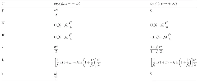
Table 1

Limiting behaviour of mean levelseY;iðq_i;uiÞand asymmetries oY;iðq_i;uiÞ ðY¼P;N;R;l;L;or a) at 0oqi¼const:oN and ui-þN(i.e.fi-þN)

Y e_Y;iðq_i;u_i-þNÞ o_Y;iðq_i;u_i-þNÞ

P e^ui

2

0

N 1

4ð2þ1=qiþqiÞ 1

4ð1=q_iqiÞ

R e^2ui

4 1qi

1þq_i e^2ui

4

l ui 1

2ð1=qiqiÞ

L 1

2ð2þ1=qiþqiÞu_i 1

2ð1=q_iqiÞu_i

a u²_i

2

0

following figures. The figures may be obtained directly from Eqs. (51)–(58) and (60)–(63); com- pressed analytical expressions for most of the different e

_Y;i

and o

_Y;i

are easily derived from these equations.

5.6. General behaviour of the even components of c

_N;i

and c

_R;i

Fig. 1 shows the different mean levels e

_Y;i

; divided by e

P;i

; as functions of u

i

at a few values of either q

i

or f

i

; for Y ¼ N and R. (We abstain from showing e

P;i

itself and e

a;i

; both of which depend in a well-known way on u

i

only.) Note the logarithmic scale on the ordinate. A comment is due concerning the values of e

Y;i

ðY ¼ N; RÞ at q

i

¼ 0: In the case of e

R;i

ðq

_i

Þ; this value coincides with the limit of e

R;i

ðq

_i

Þ for q

i

-f: The mean level e

_N;i

ðq

_i

Þ behaves anomalously. At q

_i

¼ 0; we obtain analytically e

_N;i

ðq

_i

¼ 0Þ=e

_P;i

¼ e

_R;i

ðq

_i

¼ 0Þ=e

_P;i

¼ cosh u

_i

: On the other hand, at any finite value of q

_i

a 0; e

_N;i

ðq

_i

Þ approaches a constant r

_i

¼ ð2 þ 1=q

_i

þ q

_i

Þ=4 as u

_i

- þ N (see Table 1), i.e.

e

_N;i

ðq

_i

Þ=e

_P;i

decreases as e

^ui

: Qualitatively, we can understand what is happening by noticing the behaviour of e

_N;i

ðq

_i

Þ=e

_P;i

for q

_i

¼ 0:1 and q

_i

¼ 0:01 in Fig. 1. With decreasing q

i

; the relative mean level e

N;i

ðq

_i

Þ=e

_P;i

snuggles ever more closely up to

cosh u

_i

for small u

_i

-values, only to plunge below 1 at ever larger u

_i

: Analytically we obtain

e

_N;i

ðq

_i

Þ X e

_P;i

for 0 o q

_i

p 3 ffiffiffi p 8

and

0 p u

i

o u

m;i

ð68Þ

Table 2

Limiting behaviour of mean levelse_Y;iðf_i;u_iÞand asymmetrieso_Y;i ðf_i;u_iÞ ðY¼P;N;R;l;L;or a) at 0of_i¼const:oNandu_i-þN (i.e.qi-0)

Y eY;iðfi;ui-þNÞ oY;iðfi;ui-þNÞ

P e^ui

2

0

N ð1=fiþfiÞe^ui

4 ð1=fifiÞe^ui

4

R ð1=f_iþf_iÞe^ui

4 ð1=f_if_iÞe^ui

4

l e^ui

2

1fi

1þf_i e^ui

2

L 1

f_ilnð1þfiÞ þfiln 1þ1 f_i

e^ui 2

1

f_ilnð1þfiÞ filn 1þ1 f_i

e^ui 2

a u²_i

2

0

Fig. 1. Mean levels e_Y;iðq_i;u_iÞ and e_Y;iðf_i;u_iÞof reduced chi- square quantities c_Y;i for Y¼N and R divided by e_P;i¼ coshu_i1:a) Nðf_i-0 orq_i-0Þand R (anyq_i). b) N and R ðf_i¼0:01Þ: c) N and R ðf_i¼0:1Þ: d) N and R ðf_i¼1Þ:

e) Nðq_i¼0:01Þ:f ) Nðq_i¼0:1Þ:g) Nðq_i¼1Þ:

with

u

m;i

¼ lnðh

_i

ffiffiffiffiffiffiffiffiffiffiffiffiffi h

²_i

1 q

Þ ð69Þ

h

_i

¼ ð1 q

i

Þ

²

4q

_i

: ð70Þ

Otherwise

e

_N;i

ðq

_i

Þ p e

_P;i

: ð71Þ

Incidentally, this example should caution against a cavalier treatment of multiple limiting processes which are not commuting, in general. An analo- gous case is that of e

_N;i

ð f

_i

Þ=e

_p

¼ e

_R;i

ð f

_i

Þe

_p

- 1=

ð2f

_i

Þ for large values of u

_i

and f

_i

- f:

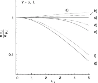
5.7. General behaviour of the even components of c

_l;i

and c

_L;i

Fig. 2 shows e

Y;i

=e

P;i

for Y ¼ l and L: The scale on the ordinate comprises two decades instead of the four decades of Fig. 1 which means that, on the average over all variables, e

l;i

and e

L;i

are about two orders of magnitude closer to e

P;i

than e

N;i

and e

R;i

: Even more remarkable is the closely similar behaviour of e

l;i

and e

L;i

: The straight line at e

Y;i

=e

P;i

¼ 1 in Fig. 2 is valid for Y ¼ l and any value of f

_i

but also for Y ¼ L at f

_i

- 0: This checks

with Table 2. However, Table 1 contradicts the hypothesis that it could be strictly valid for q

i

- 0 and either Y ¼ l or L: The example of Y ¼ N and small q

i

of Fig. 1 suggests what happens. As q

i

-0;

e

Y;i

ðq

_i

Þ=e

_P;i

(Y ¼ l or L) approaches the value of 1 for a restricted range of u

i

; say u

i

o 5; in the sense that for any positive value e o 1 a sufficiently small positive value of q

i

¼ q

i

ðeÞ can be found such that 1 eoe

Y;i

ðq

_i

Þ=e

_P;i

o1 for any u

i

o5: However, at u

_i

-values beyond the order of magnitude of ln q

_i

ðeÞ; the relative mean level e

_Y;i

ðq

_i

Þ=e

_P;i

tends to zero.

5.8. General behaviour of the odd components of c

_Y;i

Fig. 3 shows the relative asymmetries o

Y;i

=e

Y;i

(not o

Y;i

=e

P;i

Þ for Y ¼ R; l; and L: Here the scale on the ordinate is linear. Note again the close similarity between Y ¼ l and L: Note also that o

N;i

=e

N;i

¼ o

_R;i

=e

R;i

; both at given q

i

and at given f

_i

(cf. Eqs. (52)–(53)). Of course, the asymmetries are zero for Y ¼ P and a. They also vanish at q

_i

¼ 1 or at f

_i

¼ 1 for any Y (cf. Eq. (67)). The limits q

_i

- 0 and f

_i

- 0 behave normally in the sense that the limiting values of o

_Y;i

=e

_Y;i

are equal to their

Fig. 2. Same asFig. 1but forY¼l(full curves) andY¼L (dashed curves). a) Lðfi¼1Þ:b) L ðfi¼0:1Þ:c)l(anyfi or qi-0) and Lðfi-0 or qi-0). d) Lðqi¼0:01Þ:

e)lðqi¼0:01Þ:f) Lðqi¼1Þ:g)lðqi¼1Þ:

Fig. 3. Relative asymmetries o_Y;iðq_i;u_iÞ=e_Y;iðq_i;u_iÞ and o_Y;iðf_i;u_iÞ=e_Y;iðf_i;u_iÞof reduced chi-square quantitiesc_Y;i for Y¼R andl(full curves), andY¼L (dashed curves). a)land Lðfi-0 orqi-0Þ:b)lðfi¼0:3Þ:c) Lðqi¼0:3Þ:d) Lðfi¼ 0:3Þ:e)lðqi¼0:3Þ:f) allYðfi¼1 orqi¼1Þ:g) Rðqi¼0:3Þ:

h) Rðfi¼0:3Þ:i) Rðfi-0 orqi-0Þ: