New methods for generating significance levels from multiply-imputed data
Dissertation
zur Erlangung des akademischen Grades
eines Doktors der Sozial- und Wirtschaftswissenschaften (Dr. rer. pol.)
an der Fakult¨at Sozial- und Wirtschaftswissenschaften der Otto-Friedrich-Universit¨at Bamberg
vorgelegt von Christine Licht
aus Apolda
Bamberg, Oktober 2010
Date of the defence: 2010-12-10
Prof. Dr. Susanne Raessler (1st referee) Prof. Dr. Donald B. Rubin (2nd referee)
Acknowledgments
First, I would like to thank my advisors Susanne R¨assler and Donald B. Rubin for their support. Susanne R¨assler introduced me to missing-data problems and in- vited me to join the world of multiple imputation. She attended my first steps in this field and prepared me meeting and finally doing research with Donald B. Ru- bin, the ”father” of multiple imputation. He also is the ”father” of this thesis, since his incredible previous and current ideas and the close co-operation with him are the fundament of this thesis. I would like to thank him for the uncountable lessons in multiple imputation theory, for his patience, when he answered all my more or less smart questions, for inviting me to do research at the Harvard Statistics department, and in general for the whole support of this thesis.
I am very greatful to Holger Aust, who supported me whenever it was needed and beyond. He motivated me in difficult times, when no solution of the tricky problems was in sight. He shared the great moments of success with me and he always believed in me. He inspired me in many precious discussions on the topic and he made a lot of very helpful comments and corrections concerning this thesis.
He attended and supported me carringly the last three years in all areas of life, even when he was just cooking pasta, while I was writing on this thesis.
I am very thankful to my parents for their wonderful support and care. They were always interested in the progress of my work and helped me whenever they could.
Last but not least I would like to thank Julia Cielebak, who shared the office with me, for all the inspiring professional talks and especially for the wonderful ”girls- topics” talks that always lighten up the long days in the office.
Bamberg, Oktober 2010 Christine Licht
Contents
1 Introduction 3
2 Multiple imputation 6
3 Significance levels from multiply-imputed data 9 3.1 Significance levels from multiply-imputed data using moment-based
statistics and an improvedF-reference-distribution . . . . 9
3.2 Significance levels from multiply-imputed data using parameter es- timates and likelihood-ratio statistics . . . 12
3.3 Significance levels from repeated p-values with multiply-imputed data . . . 14
4 z-transformation procedure for combining repeated p-values 16 4.1 The newz-transformation procedure . . . 16
4.2 z-test . . . 17
4.3 t-test . . . 22
4.4 Wald-test . . . 26
5 How to handle the multi-dimensional test problem 31 5.1 Idea . . . 31
5.2 Simulation study . . . 32
5.3 Further problems . . . 35 6 Small-sample significance levels from repeated p-values using a compo-
6.1 Small-sample degrees of freedom with multiple imputation . . . 39 6.2 Significance levels from multiply imputed data with small sample
size based onS˜d . . . 40 7 Comparing the four methods for generating significance levels from
multiply-imputed data 44
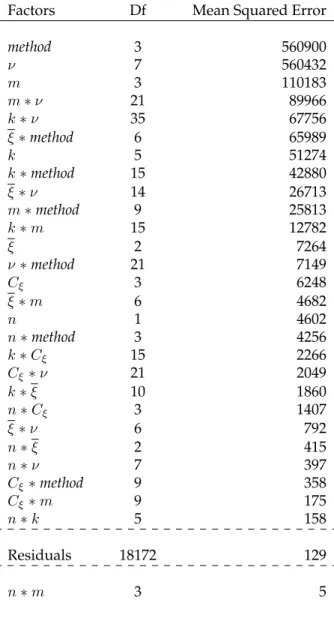
7.1 Simulation study . . . 44 7.2 Results . . . 49 7.2.1 ANOVA . . . 49 7.2.2 Combination of method and appropriate degrees of
freedom . . . 55 7.2.3 Rejection rates . . . 61 7.2.4 Conclusions . . . 78
8 Summary and practical advices 81
9 Future tasks and outlook 85
List of figures 87
List of tables 89
A Derivation of (3.1)-(3.5) from Section 3.1 92
B Derivation of the degrees of freedomδandwin the moment-based
procedure described in Section 3.1 97
References 101
1
Introduction
Missing data are an ubiquitous problem in statistical analyses that has become an important research field in applied statistics because missing values are frequently encountered in practice, especially in survey data. Many statistical methods have been developed to deal with this issue. Substantial advances in computing power, as well as in theory, in the last 30years enables the application of these methods for applied researchers. A highly useful technique to handle missing values in many settings is multiple imputation, which was first proposed by Rubin (1977, 1978) and extended in Rubin (1987). The key idea of multiple imputation is to replace the missing values with more than one, say m, sets of plausible values, thereby generating m completed data sets. Each of these completed data sets is then analyzed using standard complete-data methods. These repeated analyses are combined to create one imputation inference, that takes correctly account into the uncertainty due to missing data. Multiple imputation retains the major advantages and simultaneously overcomes the major disadvantages inherent in single imputation techniques.
Due to the ongoing improvement in computer power in the last10years, multiple imputation has become a well known and often used tool in statistical analyses.
Multiple imputation routines are now implemented in many statistical software packages. However, there still exists a problem in generally obtaining significance levels from multiply-imputed data, because Rubin’s combining rules (1978)
for the completed-data estimates require normally distributed or t-distributed complete-data estimators. Some procedures were offered in Rubin (1987), but they had limitations. Today there are basically three methods that extend the suggestions given in Rubin (1987). First, Li, Raghunathan, and Rubin (1991) pro- posed a procedure, where significance levels are created by computing a modified Wald-test statistic which is then referred to an F-distribution. This procedure is essentially calibrated and the loss of power due to a finite number of imputations is quite modest in cases likely to occur in practice. But this procedure requires access to the completed-data estimates and their variance-covariance matrices.
The full variance-covariance matrix may not be available in practice with standard software, especially when the dimensionality of the estimand is high. This can easily occur, e.g., with partially classified multidimensional contingency tables.
Second, Meng and Rubin (1992) proposed a complete-data two-stage-likelihood- ratio-test-based procedure, which was motivated by the well-known relationship between the Wald-test statistic and the likelihood-ratio-test statistic. In large samples this procedure is equivalent to the previous one and only requires the complete-data log-likelihood-ratio statistic for each multiply-imputed data set.
However, common statistical software does not provide access to the code for the calculation of the log-likelihood-ratio statistics in their standard analyses rou- tines. Third, Li, Meng, Raghunathan, and Rubin (1991) developed an improved version of a method in Rubin (1987) that only requires the χ2k-statistics from a usual complete-data Wald-test. These statistics are provided by every statistical software. Unfortunately, this method is only approximately calibrated and has a substantial loss of power compared to the previous two.
To sum, there exist several relatively ”easy” to use procedures to generate sig- nificance levels in general from multiply-imputed data, but none of them has satisfactory applicability due to the facts mentioned above. Since many statistical analyses are based on hypothesis tests, especially on the Wald-test in regression analyses, it is very important to find a method that retains the advantages and overcomes the disadvantages of the existing procedures, just as multiple imputa- tion does with the existing techniques to handle missing data. Developing such a method was the aim of the present thesis, that results from a close co-operation
with my advisor Susanne Raessler and especially with my second advisor - the
”father” of multiple imputation - Donald B. Rubin.
In Chapter 2 we briefly introduce the multiple imputation theory and give some important notations and definitions. In Chapter 3 we describe in detail the three existing procedures mentioned above that create significance levels from multiply-imputed data. In Chapter 4 we present a new procedure based on a z-transformation. First we examine this new z-transformation-based procedure for simple hypothesis tests like the z-test in Section 4.2 and the t-test in Section 4.3, before we consider the Wald-test in Section 4.4. Despite the success of this newz-transformation procedure in several practical settings, problems arise when two-sided tests are performed. Therefore we develop and discuss a possible solution in the first section of Chapter 5. Based on a comprehensive simulation study described in Section 5.2, in Section 5.3 we discover an interesting general statistical problem: Using a χ2k-distribution rather than an Fk,n-distribution, can lead to a not negligible error for small sample sizesn, especially with largerk. This problem seems to be unnoticed until now. In addition, we show the influence of the sample size for generating accurate significance levels from multiply imputed data. Due to these problems described in Chapter 5, in Chapter 6 we present an adjusted procedure, the componentwise-moment-based method, to easily calculate correct significance levels from multiply-imputed data under some assumptions. In Chapter 7 we examine this new componentwise-moment-based method and the already existing procedures in detail by an extensive simulation study and compare them with each other. We also compare the results with former simulation studies of Li, Raghunathan, and Rubin (1991), and Li, Raghunathan, Meng, and Rubin (1991), where they simulated draws from the theoretically calculated distributions of the test statistics, because it was too computationally expensive to generate data sets and impute them several times due to the lack of computer power at that time. Our simulation study enables us to give some practical advices in Chapter 8 about how to calculate correct significance levels from multiply-imputed data. Finally in Chapter 9, an overview is given for
2
Multiple imputation
Multiple imputation is a general statistical technique for handling missing data. It was developed by Rubin (1978) and is described in detail in Rubin’s book (1987) on multiple imputation. The key idea is to replace the set of missing values with m ≥ 2 sets of draws from the posterior predictive distribution of the missing data. Each of these m completed data sets can now be analyzed using standard complete-data techniques, thereby resulting inmcompleted-data statistics. These are combined to form one multiple imputation inference, which takes account of the uncertainty due to nonresponse or in general missing data.
Let θ be the quantity of interest in the data set, for example a k-component regression coefficient vector from a simple least squares regression. If there were no missing data, we assume that
(ˆθ−θ)∼N(0, U), (2.1)
where θˆis the estimate of θ with associated variance-covariance matrix U pro- duced by using standard complete-data analysis. Suppose now thatmcompleted data sets were created by drawing m repeated imputations. Let θˆ∗1, . . . ,θˆ∗m de- note the m values for θ,ˆ U∗1, . . . , U∗m the m associated variance-covariance ma- trices, and Sm = {(ˆθ∗l, U∗l), l = 1, . . . , m} the collection of completed-data mo- ments. The mrepeated completed-data estimates and associated completed-data
(within) variance-covariance matrices can be combined using Rubin’s (1987) com- bining rules. Let
θm= 1 m
m
X
l=1
θˆ∗l (2.2)
be the average of themcompleted-data estimates, let Um = 1
m
m
X
l=1
U∗l (2.3)
be the average of themcompleted-data variance-covariance matrices, and let Bm = 1
m−1
m
X
l=1
(ˆθ∗l−θm)t(ˆθ∗l−θm) (2.4)
be the between variance of themcompleted-data estimates. The total variance of (θm−θ)is defined to be
Tm =Um+ (1 +m−1)Bm. (2.5)
Ifθ is a scalar, Rubin (1987) showed that, approximately
(θm−θ)∼tν(0, Tm), (2.6)
with
ν = (m−1)(1 +rm−1)2 (2.7) degrees of freedom, where rm is the relative increase in variance due to nonre- sponse:
rm = (1 +m−1)Bm/Um. (2.8) If θ is a k-dimensional vector, (2.2)-(2.7) still hold approximately withrm in (2.8) generalized to be the average relative increase in variance due to nonresponse
rm = (1 +m−1)Tr(BmU−1m )/k, (2.9)
where Tr(A)denotes the trace of the matrixA.
The fraction of missing information is defined as
γm= [U−1m −(ν+ 1)(ν+ 3)−1Tm−1]·Um, (2.10)
where for scalarθ we obtain
γm = rm+ 2/(ν+ 3)
rm+ 1 . (2.11)
For calculating significance levels based on the combined estimates and variance- covariance matrices, whenmis modest relative tokwe use the statistic
D˜m = (1 +rm)−1(θm−θ0)U−1m (θm−θ0)t/k (2.12)
where θ0 is the null value ofθ. In Rubin (1987) the statistic D˜m is referred to an F-distribution onkand(k+ 1)ν/2degrees of freedom.
3
Significance levels from multiply-imputed data
3.1 Significance levels from multiply-imputed data using moment-based statistics and an improved F - reference-distribution
Li, Raghunathan, and Rubin (1991) presented an improved procedure for creating significance levels based on the set of completed-data moments. To start with, we provide some further notation, which we need throughout this thesis.
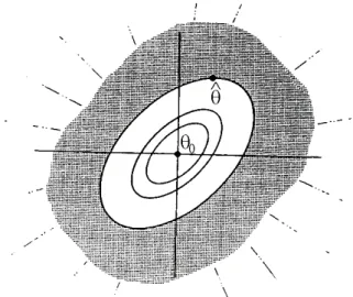
Let θt be the true value of the k-dimensional parameter of interest and let θˆobs be the maximum-likelihood estimate ofθ based on the observed data. Let Ut denote the true variance of the complete data, that is,Ut =V(ˆθ|θ =θt), andUt−1 is the complete-data information. Tt = V(ˆθobs|θ = θt)describes the true variance of θˆobsandTt−1 is the observed information. The subscriptstonθ,U, andT designate the true values ofθ,U, andT. Then
Bt=Tt−Ut
is the increase in variance due to nonresponse and the missing information is Ut−1 −Tt−1. Thus the ratios of missing to observed information are given by the
relative toUt, which we label by(λ1, . . . , λk)∈[0,∞)k, since each symmetric matrix can be characterized by their real eigenvalues. The ratios of complete to observed information are given by
ξi = (1 +λi), i= 1, . . . , k, (3.1)
and the ratios of missing to complete information, that is, the fractions of missing information,γi, based on the true variances are given by the eigenvalues of(Ut−1− Tt−1)Ut. In additionξi = (1 +λi) = (1−γi)−1. Furthermore, letCξbe the coefficient of variation of theξidefined as
1 +Cξ2 = 1 k
k
X
i=1
(ξi/ξ)2, (3.2)
whereξ= 1k
k
P
i=1
ξidenotes the average ratio of complete to observed information.
The procedure proposed by Li, Raghunathan, and Rubin (1991) is based on the test statisticD˜m from (2.12) withθm, Um and rm defined in Chapter 2. They show (Li, Raghunathan, and Rubin (1991), page 1069) thatD˜min (2.12) can be written as
D˜m =
k
P
i=1
θ2m,i/k
1 +rm (3.3)
with
rm = (1 +m−1)
k
X
l=1 m
X
l=1
(ˆθ∗l−θm)2/k(m−1) (3.4)
under certain assumptions, especially if the sample size is large. They derive the distribution ofD˜m as
D˜m ∼ χ2k/k
(1 +aχ2b/b)/(1 +a), (3.5) whereb = k(m−1)anda = (1 +m−1)λunder the equal eigenvalue assumption, that is, λi = λ. Note, that the derivations of (3.1)-(3.5) are given in Appendix A. Li, Raghunathan, and Rubin (1991) improved a procedure in Rubin (1987) by
using a moment matching method to approximate the distribution of D˜m in (3.5) by a multiple of anF-distribution,δFk,w. Calculating the Taylor-series expansion of (3.5) in 1/χ2b around its expectation, 1/(b−2) and then matching the first two moments of that expansion with the first two moments of theF-distribution, gives
δ= (1−2/w)[1 +ab/(b−2)]/(1 +a) = (1−2/w)· b(1 +a)−2
b(1 +a)−2a−2, (3.6) and
w= 4 + (b−4)[1 + (1−2b−1)/a]2 = 4 + (b−4)
1 + b−2 ab
2
. (3.7)
Note that with our calculation, which is given in Appendix B, we get similar, but not identical degrees of freedom:
δ0 = (1−2/w)· b(1 +a)
b(1 +a)−2a and w0 = 4 + (b−4)
1 + b a(b−2)
2
.
Unfortunately, we could not derive the degrees of freedom given in Li, Raghu- nathan, and Rubin (1991), and thus it is not possible to show where the difference comes from. Nevertheless, all our simulations described in the following chapters use the original degrees of freedom δ and w. First, the difference between (δ, w) and(δ0, w0)is not that important: alsoδ0 is also approximately1, andwand w0 are often very large. Second, all their simulation studies and conclusions were based on their degrees of freedom and we want on the one hand to reproduce and on the other hand to compare their results in our simulation study (Chapter 7) with our new ”componentwise-moment-based” procedure.
Based on the derivation of δ and w, they consider the behavior of D˜m also with unequal ratios of complete to observed information. Moreover, they examine the loss of power for finite m as well as for infinitem. For m → ∞they showed that D˜m is essentially the same as the ideal procedure - the two-stage-likelihood- ratio-test based directly on the observed data. In addition to their analytical calculations, they run several simulation studies where they, due to the processing power of the computers at that time, use repeated draws from theχ2-distributions
in (3.5) and compare the associated levels with the nominal levels. In Chapter 7 we will calculate values ofD˜mdirectly from generated multiply-imputed data.
They finally conclude that their procedure based on D˜m is essentially well calibrated and has no substantial loss of power except in relatively extreme circumstances, as for example with a large variation in the fractions of missing information.
The disadvantage of this procedure is that it requires access to the collection of completed-data moments Sm = {(ˆθ∗l, U∗l), l = 1, . . . , m}and the inverse of the within variance-covariance matrix Um. Because of recent computer power and depending on the dimension k of the estimand, it might not be an intractable problem in some settings to calculate the inverse of the within variance-covariance matrix, but standard analysis software does usually not provide the set of completed-data moments,Sm.
3.2 Significance levels from multiply-imputed data using parameter estimates and likelihood-ratio statistics
Motivated by the well-known relationship between the Wald-test statistic and the likelihood-ratio-test statistic, Meng and Rubin (1992) suggested a procedure that does not require the variance-covariance matrices, U∗l. Yet it needs access to the code for the complete-data log-likelihood-ratio statistic as a function of parameter estimates for each data set completed by multiple imputation. They assume that the complete-data analysis provides theχ2k-distributed test statistic of a likelihood-ratio-test, that can be evaluated at new values.
As introduced in Chapter 2,θ denotes the parameter of interest. In addition, there usually will be nuisance parameters φ, which include all other parameters of the analysis. For example, let X be an (n × k)-data matrix where Xi (i = 1, . . . , k)
denotes theith column vector ofX, and letY denote the outcome variable. When setting all of thek regression coefficients,θ, of the linear regression model
Y =θ0+Xθ+=β0 +θ1X1. . .+θkXk+,
where each component ofis independent, identically distributed with zero mean and common varianceσ2, equal to zero,φ includes the estimates of the intercept and the residual variance of the null model. That is, the nuisance parametersφare estimated by different values when θ = ˆθ and θ = θ0, respectively. Let φˆdenote the complete-data estimate ofφwhen θ = ˆθand φˆ0 be the complete-data estimate ofφ when θ = θ0. For the following procedure, Meng and Rubin (1992) suppose that the complete-data analysis of each of the m imputed data sets produces the estimates (ˆθ,φ)ˆ , the null estimates (θ0,φˆ0), and the χ2-statistic of the likelihood- ratio-test,d. Consider this complete-dataχ2-statistic as a function of(ˆθ,φ)ˆ, (θ0,φˆ0) and the data set, sayd(ˆθ,φ, θˆ 0,φˆ0). In our regression example we have
d(ˆθ,φ, θˆ 0,φˆ0) =d( ˆβ,σˆ2,βˆ0,σˆ20) =−2(LL1−LL0), with
LL1( ˆβ,σˆ2|Y, X) = −n2 ·ln(2π)− n2 ·ln(ˆσ2)−2ˆ1σ2
·(Y −βˆ0−βˆkX1−. . .−βˆkXk)2, LL0( ˆβ0,σˆ2
0|Y, X) = −n2 ·ln(2π)− n2 ·ln(ˆσ2
0)− 2ˆσ12 0
·(Y −βˆ0)2,
where {Y, X} denotes the given (completed) data set with X1, . . . , Xk as the independent variables, on whichY is regressed.
Let θ, φ, φ0, and d denote the average values of θ,ˆ φ,ˆ φˆ0, and d across the m imputations. Assume that the function d can be evaluated at θ, φ, θ0, and φ0 for each of the m completed data sets to obtain m values of d(θ, φ, θ0, φ0), whose average across themimputations isd∗. Then the repeated-imputation p-value is
p-value = Prob(Fk,w>D),˘ where
andFk,wis an F-random variable on kand wdegrees of freedom, wherek equals the number of components ofθ, andwequals the denominator degree of freedom of the moment-based procedure given by (3.7).
Meng and Rubin (1992) show that for large samples, their two-stage-likelihood- ratio-test-based method is equivalent to the moment-based procedure for any number of multiple imputations. Instead of requiring the variance-covariance matrices and the inverse of the within variance-covariance matrix, that is a difficult problem especially when the dimensionality of the estimand is high, the two-stage-likelihood-ratio-test-based procedure requires only the point estimates and evaluations of the complete-data log-likelihood-ratio statistic as a function of these estimates and the completed data. The disadvantage of this procedure is, that none of the today’s common statistical software packages provide access to the code for evaluating the complete-data log-likelihood at user-specified values of the parameters, although it is easy and fast to calculate and implement, and it does not involve the computation of any matrices.
3.3 Significance levels from repeated p-values with multiply-imputed data
Both of the above described procedures inherently have the problem that espe- cially for practical problems with hundreds of variables the standard complete- data analysis provides the collection of completed-data χ2k-statistics Sd = {d∗1, . . . , d∗m}with
d∗l = (θ0−θˆ∗l)tU∗l−1(θ0−θˆ∗l) (3.9) but not the collection of completed-data moments Sm or the likelihood-ratio-test statistic d(θ, φ, θ0, φ0). The problem of directly combining {d∗l, l = 1, . . . , m}
according to (2.2) is difficult, because Rubin’s combining rules require normally distributed ort-distributed estimators, butd∗lisχ2k-distributed. Disregarding that fact and combiningd∗ldirectly, leads to too significant p-values.
Li, Meng, Raghunathan, and Rubin (1991) proposed a procedure for creating significance levels based onSdrather thanSm. They use the fact that Rubin (1987) showed that (2.12) implies
D˜m ≈Dˆm = dmk−1 −(m−1m+1)rm
1 +rm , (3.10)
where dm is the sample mean of {d∗l, l = 1, . . . , m} and rm is given by (2.9). Re- placingrm inDˆm with estimates obtained from the set Sdrather than Sm leads to procedures for calculating p-values when onlySdis given. A suggestion of Rubin (1987) provides accurate levels ifm ≥k, which in practice often is impossible, and a modest fraction of missing information. Therefore Li, Meng, Raghunathan, and Rubin (1991) proposed the following replacement ofrm by the estimaterˆdwith
ˆ
rd = (1 +m−1)[ 1 m−1
m
X
l=1
(p
d∗l−√
d)2], (3.11)
that is, rˆd is the sample variance of √
d∗1, . . . ,√
d∗m times (1 −m−1). The corre- sponding test statistic Dˆˆd is of the form Dˆm from (3.10) with rm replaced by the estimate rˆdfrom (3.11). As reference distribution they use an F-distribution onk andak,mwsdegrees of freedom, where
ws = (m−1)(1 + ˆrd−1)2 (3.12) and
ak,m=k−3/m. (3.13)
The obvious advantage of this procedure is that only the completed-data test statistics,{d∗l, l= 1, . . . , m}, are needed for computing the p-value and it is simple to apply. But the procedure is only approximately calibrated and has a substantial loss of power compared toD˜m. The problem with this method and other methods based on Sd, as shown for example in Li (1985) and Raghunathan (1987), is that the loss of information usingSdinstead ofSmis too big.
4
z -transformation procedure for combining repeated p-values
In 2009 Rubin came up with an idea for combining p-values from multiply- imputed data directly, using a simple transformation and his usual combining rules introduced in Chapter 2. In the following sections we will describe and explore behavior and possibilities of this new procedure, which we call the z- transformation procedure.
4.1 The new z -transformation procedure
Suppose the standard complete-data analysis of multiply-imputed data provides the collection of statisticsSs ={s∗1, . . . , s∗m}of an arbitrary hypothesis test and/or the set of the corresponding p-valuesSp ={p∗1, . . . , p∗m}, where
p∗l = Prob(reference distribution ≥s∗l), l= 1, . . . , m. (4.1)
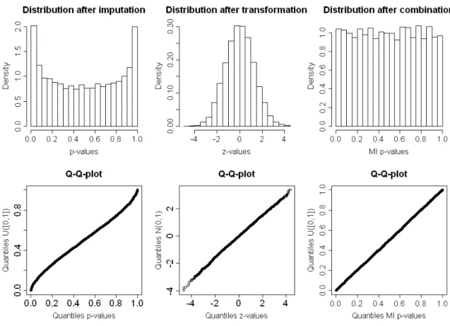
As described in Section 3.3 we cannot combine these p-values directly to get valid inferences, because under the null hypothesis these p-values are uniformly distributed and Rubin’s combining rules require a normal distribution or a t-distribution. The idea is to transform the p-values to a normal distribution using the quantile functionΦ−1 of the standard normal distribution.
Let Sz = {z∗l, l = 1, . . . , m} be the collection of the transformed completed- data p-values, where
z∗l= Φ−1(1−p∗l). (4.2)
After this transformation we calculate the multiple imputation estimatorzmas av- erage over the transformed test statisticsz∗las
zm = 1 m
m
X
l=1
z∗l, (4.3)
and the between varianceBmgiven in (2.4) as Bm = 1
m−1
m
X
l=1
(z∗l−zm)t(z∗l−zm). (4.4)
Because of the z-transformation, the within variance Um given in (2.3) equals 1.
Thus, the total varianceTm given in (2.5) is calculated as
Tm=Um+ (1 +m−1)Bm = 1 + (1 +m−1)Bm. (4.5) It follows from (2.6) that the multiple imputation estimator zm is tν(0, T)- distributed withν given in (2.7). The corresponding p-value
pm = Prob(tν(0, T)≥zm) (4.6) is the intended p-value for multiply-imputed data, which is produced just by using this simple transformation and the setSdorSp, respectively.
The interesting question is how well this simple procedure performs and for which settings it will be applicable.
4.2 z -test
First we consider a simple hypothesis test - a one-sided z-test, for example a two
tributed population with known variance is less than or equal to the mean of a second normally distributed population both with known variance. The corre- sponding test statistic is
S = X1X2 qσ21
n1 +σn22
2
∼N(0,1), (4.7)
whereX1andX2 are the sample means andn1andn2are the sample sizes.
In addition we choose a simple model for the following calculations. Let X be a random sample of size n with each component of X distributed asN(0,1).
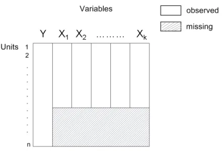
X(1) denotes the first half ofX with sizen(1) = n/2andX(2) the second half ofX with sizen(2) =n(1) =n/2. Now we randomly delete the firstn(1)mis = n2·γ values of X(1), whereγ denotes the missingness-rate, which in this case equals the fraction of missing information defined in Chapter 2. Furthermore denote the observed part ofXbyXobs, the missing values byXmisand the observed part ofX(1)byXobs(1) and the missing values ofX(1)byXmis(1), respectively, as shown in Figure 4.1.
Figure 4.1:Example of an(n×1)-data vector seperated in two subsamplesX(1)andX(2) with same sample size, where the first values ofX(1)are missing: Solid = missing, white = observed
In addition we useX(1), X(2),X(1)misandX(1)obs for the corresponding sample means.
To impute the missing values, we apply the following proper imputation model:
µ|Xobs ∼ N
X(1)obs, 1
n(1)obs
=N
X(1)obs,n·(1−γ)2 , Xmis(1)|Xobs, µ ∼ N(µ,1).
(4.8)
First of all we are interested in the distribution of thez-statistic given in (4.7) after one (single) imputation. From (4.8) we get:
X(1)mis|Xobs, µ ∼N
µ, 1
n(1)mis
=N µ,nγ2
,
X(1)|Xobs, µ−X(2) = γ·X(1)mis|Xobs, µ+ (1−γ)·X(1)obs−X(2),
∼ N
γ·µ+ (1−γ)X(1)obs−X(2),2γn ,
s∗l|Xobs, µ = X
(1)|Xobs,µ−X(2)|Xobs,µ s
σ2 (1) n(1)+
σ2 (2) n(2)
= X
(1)|Xobs,µ−X√ (2)|Xobs,µ
4 n
,
∼ N pn
4 ·
γµ+ (1−γ)X(1)obs−X(2)
,n4 · 2γn ,
= N pn
4 ·
γµ+ (1−γ)X(1)obs−X(2) ,γ2
,
s∗l|Xobs ∼ N pn
4 ·
γ·X(1)obs+ (1−γ)X(1)obs−X(2)
,γ2 + n4 ·γ2· n(1−γ)2 ,
= N pn
4 ·
X(1)obs−X(2)
,γ2 + 2(1−γ)γ2 ,
= N pn
4 ·
X(1)obs−X(2)
,2(1−γ)γ .
(4.9)
The corresponding completed-data p-valuesp∗l are calculated using the distribu- tion functionΦ(.)of a standard normally distribution
because with complete data the test statisticSgiven in (4.7) has a standard normal distribution as reference distribution. If we apply the z-transformation to thep∗l
given in (4.10) we get the transformed valuesz∗l
z∗l|Xobs = Φ−1(1−p∗l|Xobs) = Φ−1(Φ(s∗l|Xobs)) =s∗l|Xobs. (4.11)
Thus, for thez-test the test statistic,s∗l, and the test statistic after transformation, z∗l, are equal, because the reference distribution of the z-test (without missing data) is the standard normal distribution and for the z-transformation also a standard normal distribution is used.
We combine themvalues ofz∗l ors∗l, respectively given in (4.9) to zm|Xobs ∼N
rn 4 ·
X(1)obs−X(2)
, γ
2m(1−γ)
. (4.12)
BecauseX(1)obs ∼N
0,n(1−γ)2
andX(2) ∼N 0,n2
, it follows rn
4 ·
X(1)obs−X(2)
∼N
0,n 4 ·
2
n + 2
n(1−γ)
=N
0, 2−γ 2(1−γ)
. (4.13)
From (4.12) and (4.13) it follows:
zm ∼ N
0,2m(1−γ)γ +2(1−γ)2−γ ,
= N
0,2m(1−γ)γ +2−γ+γ−γ2(1−γ) ,
= N
0,2m(1−γ)γ +2−2γ+γ2(1−γ) ,
= N
0,2m(1−γ)γ +2(1−γ)+γ2(1−γ) ,
= N
0,2m(1−γ)γ + 1 + 2(1−γ)γ ,
= N
0,1 + 2(1−γ)γ (1 +m−1) ,
= N(0, Ut+Bt(1 +m−1)),
(4.14)