• Keine Ergebnisse gefunden

Generating Multiply Imputed Synthetic Datasets: Theory and Implementation

N/A
N/A
Protected

Academic year: 2021

Aktie "Generating Multiply Imputed Synthetic Datasets: Theory and Implementation"

Copied!
166
0
0

Wird geladen.... (Jetzt Volltext ansehen)

Volltext

(1)

Generating Multiply Imputed Synthetic Datasets: Theory and Implementation

Dissertation

zur Erlangung des akademischen Grades

eines Doktors der Sozial- und Wirtschaftswissenschaften (Dr. rer. pol.)

an der Fakult¨at Sozial- und Wirtschaftswissenschaften der Otto-Friedrich-Universit¨at Bamberg

vorgelegt von J¨org Drechsler

Bamberg, im Februar 2010

(2)
(3)

Datum der Disputation: 10. Dezember 2009

Pr¨ufungskommission:

1. Gutachter: Professor Dr. Susanne R¨assler

2. Gutachter: Professor Trivellore Raghunathan, Ph.D.

3. Gutachter (Disputation): Professor Dr. Henriette Engelhardt-W¨olfler

(4)
(5)

To my mother and my father (in loving memory)

for their love and support

(6)
(7)

Acknowledgements

This work would never have been possible without the help of many colleagues and friends and I am very grateful for their wonderful support. Firstly, I want to thank my advisor Susanne R¨assler for introducing me to the world of multiple imputation and suggesting to join a research project on synthetic data at the Institute for Employment Research (IAB) that finally became the corner stone of this thesis. Her remarkable enthusiasm helped me to pass some of the local minima of my dissertation function and without her I would never have met and eventually worked with some of the greatest researchers in the field.

I am very grateful to Trivellore Raghunathan for joining my dissertation com- mittee. Although I only had two weeks during a visit at the University of Michigan to benefit from his expertise, I learned a lot in that short period of time and I am still deeply impressed by his ability to understand complex research problems within seconds even when explained badly by some PhD stu- dent, but even more importantly to instantly come up with often simple and straightforward solutions for seemingly (at least for me) unsolvable problems.

I also want to thank John Abowd for inviting me to participate in the weekly video conferences with the leading experts on synthetic data in the U.S. When I started my research, I was the only one involved in that topic in Europe and following the discussions and learning from their experience during these weekly meetings was extremely helpful for my endeavor. To Don Rubin, one of the founding fathers of synthetic data, I am thankful for inviting me to present my work at Harvard and for fruitful discussions on some of my papers on the topic. Bill Winkler deserves my gratitude for providing the extensive list of references on microdata confidentiality included in the Appendix of my thesis.

At the IAB I am especially thankful to Hans Kiesl, Thomas B¨uttner, and Stefan Bender. Hans for always helping me out when my lack of background in survey statistics once again became too obvious. Thomas for joining me in the dissertation journey. It was a great relief to have a fellow sufferer. And both of them for helpful discussions on the details of multiple imputation and for unforgettable road trips framing JSMs and other conferences around the world. Stefan was very supportive for my research from the very beginning.

He stood up for my work when others were still merely laughing at the idea of

generating synthetic datasets even though he was and probably still is sceptical

(8)

about the idea himself. He helped me find my way in the jungle of official statistics and assisted me in any way he could.

My deepest gratitude is to Jerry Reiter with whom I had the pleasure to work on several projects which later became part of my thesis. Almost everything I know on the theoretical concepts behind synthetic datasets I owe to him. He has been and continues to be a great mentor and friend.

Most importantly I want to thank my mother Ursula Drechsler, her partner

Jochen Paschedag, and the rest of my family for their wonderful support and

care. Even though spending three years developing fake data must have seemed

bizarre to them, they were always interested in the progress of my work and

helped me whenever they could. Finally, I would never have survived this

trip without the constant love of my girlfriend Veronika. There is no way

I can thank her enough for all her patience and understanding for numerous

weekends and evenings I spent in front of the computer. She always cheered me

up when deadlines were approaching surprisingly fast and the simulations still

didn’t provide the results they were supposed to show. Thanks for bringing

more colors to my live.

(9)

Contents

1 Introduction 1

2 Background on Multiply Imputed Synthetic Datasets 7

2.1 The history of multiply imputed synthetic datasets . . . . 7

2.2 Advantages of multiply imputed synthetic datasets compared to other SDC methods . . . 11

3 Multiple Imputation for Nonresponse 15 3.1 The concept of multiple imputation . . . 15

3.2 Two general approaches to generate imputations for missing values 17 3.2.1 Joint modeling . . . 17

3.2.2 Fully conditional specification (FCS) . . . 18

3.2.3 Pros and cons of joint modeling and FCS . . . 20

3.3 Real data problems and possible ways to handle them . . . 21

3.3.1 Imputation of skewed continuous variables . . . 21

3.3.2 Imputation of semi-continuous variables . . . 22

3.3.3 Imputation under non-negativity constraints . . . 22

3.3.4 Imputation under linear constraints . . . 23

3.3.5 Skip patterns . . . 23

4 The IAB Establishment Panel 25 5 Fully Synthetic Datasets 29 5.1 Inference for fully synthetic datasets . . . 30

5.2 Data utility for fully synthetic datasets . . . 31

5.3 Disclosure risk for fully synthetic datasets . . . 32

5.4 Application of the fully synthetic approach to the IAB Estab- lishment Panel . . . 34

i

(10)

5.4.1 The imputation procedure . . . 36

5.4.2 Measuring the data utility . . . 37

5.4.3 Assessing the disclosure risk . . . 40

6 Partially Synthetic Datasets 47 6.1 Inference for partially synthetic datasets . . . 48

6.2 Data utility for partially synthetic datasets . . . 49

6.3 Disclosure risk for partially synthetic datasets . . . 49

6.3.1 Ignoring the uncertainty from sampling . . . 50

6.3.2 Accounting for the uncertainty from sampling . . . 52

6.4 Application of the partially synthetic approach to the IAB Es- tablishment Panel . . . 53

6.4.1 Measuring the data utility . . . 54

6.4.2 Assessing the disclosure risk . . . 55

6.5 Pros and cons of fully and partially synthetic datasets . . . 57

7 Multiple Imputation for Nonresponse and Statistical Disclo- sure Control 59 7.1 Inference for partially synthetic datasets when the original data is subject to nonresponse . . . 60

7.2 Data utility and disclosure risk . . . 61

7.3 Multiple imputation of the missing values in the IAB Establish- ment Panel . . . 61

7.3.1 The imputation task . . . 62

7.3.2 Imputation models . . . 62

7.3.3 Evaluating the quality of the imputations . . . 63

7.4 Generating synthetic datasets from the multiply imputed IAB Establishment Panel . . . 71

7.4.1 The synthesis task . . . 72

7.4.2 Measuring the data utility . . . 75

7.4.3 Caveats in the use of synthetic datasets . . . 81

7.4.4 Assessing the disclosure risk . . . 84

7.4.4.1 Log-linear modeling to estimate the number of matches in the population . . . 86

7.4.4.2 Results from the disclosure risk evaluations . . 87

7.4.4.3 Disclosure risk for large establishments . . . 88

(11)

iii 7.4.4.4 Additional protection for the largest establish-

ments in the survey . . . 91

8 A Two Stage Imputation Procedure to Balance the Risk- Utility-Trade-Off 93 8.1 Inference for synthetic datasets generated in two stages . . . 94

8.1.1 Fully synthetic data . . . 94

8.1.2 Partially synthetic data . . . 96

8.2 Data utility and disclosure risk . . . 97

8.3 Application of the two stage approach to the IAB Establishment Panel . . . 98

8.3.1 Data utility for the panel from one stage synthesis . . . . 98

8.3.2 Disclosure risk for the panel from one stage synthesis . . 99

8.3.3 Results for the two stage imputation approach . . . 104

9 Chances and Obstacles for Multiply Imputed Synthetic Datasets 107 Appendix 113 A.1 Bill Winkler’s Microdata Confidentiality References . . . 113

A.2 Binned residual plots to evaluate the imputations for the cate- gorical variables . . . 132

A.3 Simulation study for the variance inflated imputation model . . 139

(12)

iv

(13)

List of Figures

5.1 The fully synthetic approach for the IAB Establishment Panel. . 36 5.2 Included variables from the IAB Establishment Panel and the

German Social Security Data. . . 38 5.3 Occurrence of establishments already included in the original

survey by establishment size. . . 43 5.4 Distribution of the matching rates for different multiple response

questions. . . 44 5.5 Histogram of the relative difference between original and im-

puted values for the variable establishment size. . . 44 7.1 Observed and imputed data for payroll and number of partici-

pants in further education . . . 66 7.2 Model checks for turnover and number of participants in further

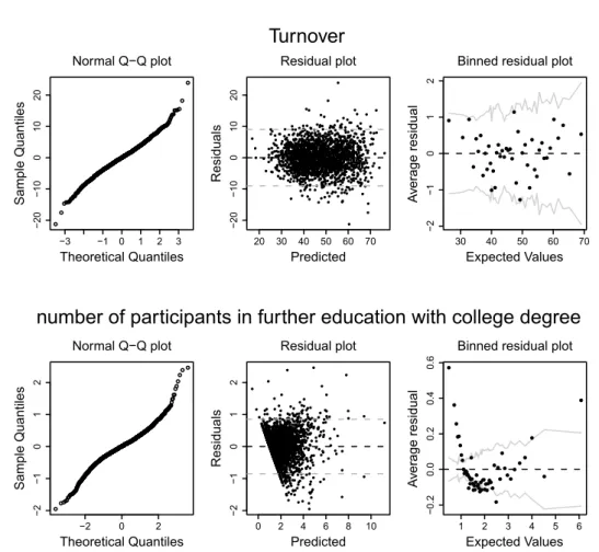
education with college degree. . . 68 7.3 Ordered probit regression of expected employment trend on 39

explanatory variables and industry dummies. . . 78 7.4 Original point estimates against synthetic point estimates for

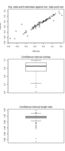
the overall mean and the means in subgroups defined by estab- lishment size class, industry code and region. . . 79 7.5 Box plots of CI overlaps for all continuous variables for the

overall mean and the means in all subgroups defined by different stratifying variables. . . 80 7.6 QQ-plots for the number of employees covered by social security

2006 and 2007 and the employment trend between the two years. 83 7.7 Plots of F t against ˆ F t for all establishments and for establish-

ments with more than 100 employees. . . 88

v

(14)

vi LIST OF FIGURES A.1 Binned residual plots for the categorical variables with missing

rates above 1%. . . 132 A.2 Binned residual plots for the categorical variables with missing

rates above 1%. . . 133 A.3 Binned residual plots for the categorical variables with missing

rates above 1%. . . 134 A.4 Binned residual plots for the categorical variables with missing

rates above 1%. . . 135 A.5 Binned residual plots for the categorical variables with missing

rates above 1%. . . 136 A.6 Binned residual plots for the categorical variables with missing

rates above 1%. . . 137 A.7 Binned residual plots for the categorical variables with missing

rates above 1%. . . 138

(15)

List of Tables

5.1 Results from the vocational training regression for one stage full synthesis. . . 39 5.2 How many records are sampled how often in the new samples? . 41 5.3 Establishments from the IAB Establishment Panel that also oc-

cur in at least one of the new samples. . . 42 6.1 Results from the vocational training regression for one stage

partial synthesis. . . 55 7.1 Missing rates and means per quantile for NB.PRE. . . 67 7.2 Expectations for the investments in 2007. . . 70 7.3 Regression results from a probit regression of part time-

employees (yes/no) on 19 explanatory variables in West Germany. 76 7.4 Regression results from a probit regression of part time-

employees (yes/no) on 19 explanatory variables in East Germany. 77 7.5 Regression results from a probit regression of employment trend

(increase/no increase) on 19 explanatory variables in West Ger- many. . . 82 7.6 Probabilities to be included in the target sample and in the

original sample depending on establishment size. . . 85 7.7 Average F t and ˆ F t for different establishment size classes. . . 87 7.8 Disclosure risk summaries for the synthetic establishment panel

wave 2007. . . 88 7.9 False match rate and true match risk for different levels of γ. . . 89 7.10 Mode of the establishment size rank and average match rate for

large establishments. . . 90 8.1 Average number of employees by industry for one stage synthesis. 99

vii

(16)

viii LIST OF TABLES 8.2 Results from the vocational training regression for one stage

partial synthesis revisited. . . 100 8.3 Confidence interval overlap for the average number of employees

for one stage synthesis. . . 101 8.4 Confidence interval overlap for the vocational training regression

for one stage synthesis. . . 102 8.5 Average confidence interval overlap for all 31 estimands for ten

independent simulations of one stage synthesis. . . 103 8.6 Averages of the disclosure risk measures over ten simulations of

one stage synthesis. . . 104 8.7 Average CI overlap and match risk for two stage synthesis based

on ten simulations. . . 105

A.1 Simulation results for the variance inflated imputation model. . 140

A.2 Simulation results if Y 1 is excluded from the imputation model. 142

(17)

Chapter 1 Introduction

National Statistical Institutes (NSIs) like the U.S. Census Bureau or the Ger- man Federal Statistical Office gather valuable information on many different aspects of the society. Broad access to this information is desirable to stimulate research in official statistics. However, most data obtained by the institutes are collected under the pledge of privacy and thus the natural interest of en- abling as much research as possible with the collected data has to stand back behind the confidentiality guaranteed to the survey respondent. But not only legal aspects are relevant when considering disseminating data to the public.

Respondents that feel their privacy is at risk might be less willing to provide sensitive information, might give incorrect answers or might even refuse to par- ticipate completely – with devastating consequences for the quality of the data collected (Lane, 2007). Traditionally, this meant that access to the data was strictly limited to researchers working for the NSI. With the increasing demand for access to the data on the micro-level from external researchers, accelerated by the improvements in computer technology, agencies started looking for pos- sibilities to disseminate data that provide a high level of data quality while still guaranteeing confidentiality for the participating units.

Over the years a broad literature on statistical disclosure limitation (SDL) techniques for microdata evolved (see Bill Winkler’s famous list of microdata confidentiality references in the Appendix A.1). These techniques can be di- vided into two main categories: Approaches that protect the data by reducing the amount of information contained in the released file through coarsening of the data and approaches classified as data perturbation methods that try to maintain most of the originally collected information but protect the data

1

(18)

2 CHAPTER 1. INTRODUCTION by changing some of the values on the micro level. Information reducing ap- proaches protect the data by

categorizing continuous variables: Building categories from the underly- ing continuous variables and reporting only in which category the unit falls, for example building age groups in five year intervals.

top coding: Setting values above a certain threshold equal to the thresh- old, for example reporting the income for all individuals with income above 100,000 as ”100,000+”

coarsening categorical variables: Coarsening to a reduced number of cat- egories, for example instead of providing information on the state level, only reporting whether a respondent lives in West or East Germany.

dropping variables: Dropping some variables that are considered too sensitive (e.g. HIV-status) or are not enough protected by any of the above methods.

There is a vast literature on data perturbation methods and discussing all approaches including possible modifications is beyond the scope of this intro- duction. A detailed overview is given in the handbook on statistical disclosure control (Center of Excellence for Statistical Disclosure Control, 2009) issued by members of the CENEX-SDC project funded by Eurostat. A good refer- ence for recent developments are the proceedings from the biannual conference Privacy in Statistical Databases (Springer LNCS 3050, 4302, 5262).

While the first methods developed in the eighties like swapping and adding noise manly focused on disclosure protection and preserved only some univari- ate statistics like the population mean and the variance of a single variable, more sophisticated methods emerged in recent years. But these sophisticated methods often require different complicated adjustments for each estimate to get unbiased results, preserve only certain statistics like the vector of the means or the variance-covariance matrix, or are valid only under specific distributional assumptions like multivariate normality that are unrealistic for real datasets.

Besides, most statistical agencies still only apply standard methods mainly be-

cause of their easy of implementation. Winkler (2007b) shows the devastating

consequences on data quality for many of these easy to implement procedures

while others fail to achieve their primary goal: protecting the data adequately.

(19)

3 Since many of the proposed data perturbation methods significantly reduce data quality and it is often impossible for the researcher using the perturbed data to judge, if the results are still at least approximately valid, there is a common mistrust among researchers against these methods. Still, strict legal requirements in many countries often force agencies to perturb their data before release, even though they know that data quality can be heavily affected.

The situation is a little different in Germany where the required disclosure pro- tection for datasets only used for scientific purposes, so called scientific use files is lower than for datasets that are available to anybody (public use files). For scientific use files, the German Federal Law on Statistics enables the release of de facto anonymous microdata. ”Factual anonymity means that the data can be allocated to the respondent or party concerned only by employing an exces- sive amount of time, expenses and manpower” (Knoche, 1993). The concept of factual anonymity takes into account a rational thinking intruder, who calcu- lates the costs and benefits of the re-identification of the data. Because factual anonymity depends on several conditions and is not further defined by law, it is necessary to estimate the costs and benefits of a re-identification for every dataset with a realistic scenario. Disseminating scientific use files under this law is much easier than under the usual requirement that a re-identification of a single unit should be impossible under any circumstance. For this reason the scientific use files available in Germany traditionally are protected using only a mixture of the non perturbative methods described above. Nevertheless, there is a common agreement that the dissemination of microdata on businesses is not possible using only non perturbative methods, since the risk of disclosure is much higher for these data than it is for microdata on individuals for several reasons:

The underlying population is much smaller for businesses than it is for individuals.

Variables like turnover or establishment size have very skewed distribu- tions that make the identification of single units in the dataset very easy.

There is a lot of information about businesses in the public domain al- ready. This information can be used to identify records in the released dataset.

The benefit from identifying a unit in an establishment survey might be

(20)

4 CHAPTER 1. INTRODUCTION higher for a potential attacker than the benefit of identifying a unit in a household survey.

In most business surveys the probability of inclusion is very high for large businesses (often close to 1) so there is no additional privacy protection from sampling for these units.

Since only few variables like turnover, region, and industry code are necessary to identify many businesses, no data on enterprizes were disseminated for many years. In 2002 a joint project of the German Federal Statistical Office, several Statistical Offices of the L¨ander and the Institute for Applied Economic Re- search started investigating the possibilities of generating scientific use files for these data applying data perturbative methods for the first time in Germany.

They came to the result that using these methods a release is possible and

disseminated several survey datasets protected by either adding multiplicative

noise or microaggregation (Statistisches Bundesamt, 2005). With the long his-

tory of releasing only unperturbed data, it is not surprising that acceptance

of these datasets was rather limited in the following years. Many users of

these data tend to believe the collected data is the direct truth and ignore all

the additional uncertainty and possible bias introduced on the collection stage

by measurement errors, coding mistakes, bad sampling design and especially

steadily increasing nonresponse rates that make the implicit assumption of a

missingness pattern that is missing completely at random (Rubin, 1987) of

complete case analysis more and more questionable. The additional bias in-

troduced by the perturbation method might be dwarfed by the bias already

inherent in the data due to these facts. But also the selected perturbation

methods might be a reason for the limited acceptance. Winkler (2007b) il-

lustrates the negative consequences of univariate microaggregation, namely

on correlations and although correction factors for estimations based on data

perturbed by multiplicative noise are illustrated in the German Handbuch zur

Anonymisierung wirtschaftsstatistischer Mikrodaten (Statistisches Bundesamt,

2005) for the linear model and the SIMEX Method (Lechner and Pohlmeier,

2005) can be used for nonlinear models, both are difficult to compute and

are applicable only under some additional assumptions. The Handbuch shows

that the SIMEX method produces biased results for a probit regression us-

ing simulated data. A further disadvantage the two methods share with most

data perturbative methods is that logical constraints between variables are not

(21)

5 preserved.

This illustrates the common dilemma for data disseminating agencies: Fulfill- ing only one goal – no risk of disclosure or high data quality – is straightforward;

release data generated completely at random or release the original unchanged data. In both cases at least one party will be unhappy about the results, but balancing the two goals is extremely difficult. A dataset that guarantees the confidentiality of the respondent but is not accepted by the research commu- nity due to data quality concerns is of little value and the question arises, if the high costs in time and money to produce these datasets are justified.

A new approach to address the trade-off between data utility and disclosure risk overcoming the problems discussed above was proposed by Rubin (1993):

The release of multiply imputed synthetic datasets. Specifically, he proposed that agencies (i) randomly and independently sample units from the sampling frame to comprise each synthetic dataset, (ii) impute unknown data values for units in the synthetic samples using models fit with the original survey data, and (iii) release multiple versions of these datasets to the public. These are called fully synthetic datasets.

However, the quality of this method strongly depends on the accuracy of the model used to impute the ”missing” values. If the model doesn’t include all the relationships between the variables that are of interest to the analyst or if the joint distribution of the variables is misspecified, results from the synthetic datasets can be biased. Furthermore, specifying a model that considers all the skip patterns and constraints between the variables in a large dataset can be cumbersome if not impossible. To overcome these problems, a related approach suggested by Little (1993) replaces observed values with imputed values only for variables that bear a high risk of disclosure or for variables that contain especially sensitive information, leaving the rest of the data unchanged. This approach, discussed as generating partially synthetic datasets in the literature, has been adopted for some datasets in the US (Abowd and Woodcock, 2001, 2004; Kennickell, 1997; Abowd et al., 2006).

The aim of this book is to give the reader a detailed introduction to the dif-

ferent approaches to generating multiply imputed synthetic datasets (MISD)

by combining the theory with illustrative examples using a real dataset, the

German IAB Establishment Panel. We start by giving an overview of the

history on synthetic datasets and discussing the major advantages of this ap-

proach compared to other perturbation methods. Since the method is based on

(22)

6 CHAPTER 1. INTRODUCTION the ideas of multiple imputation (Rubin, 1978), the next chapter recapitulates its basic concepts originally proposed to impute values missing due to nonre- sponse. Advantages and disadvantages of the two major imputation strategies (joint modeling and fully conditional specification (FCS)) are also addressed.

The Chapters 5-8 on different synthetic data generation approaches are all or- ganized in the same manner. First, the general ideas of the specific approach are discussed, then the point and variance estimates that provide valid infer- ences in this context are presented. Each section concludes with an extensive application to a real dataset. Since all applications are based on the German IAB Establishment Panel, this dataset is introduced in a separate chapter at the beginning of the main part of the book (Chapter 4). The discussed data generation approaches include generating fully synthetic datasets (Chapter 5), generating partially synthetic datasets (Chapter 6), and generating synthetic datasets when the original data is subject to nonresponse (Chapter 7).

Chapter 8 contains an extension to the standard synthetic data generation to

better address the trade-off between data utility and disclosure risk: Imputa-

tion in two stages, where variables that drive the disclosure risk are imputed

less often than others. Since in general data quality and disclosure risk both

increase with the number of imputations, defining a different number of impu-

tations for different variables can lead to datasets that maintain the desired

data quality with reduced risk of disclosure. In this chapter, the new com-

bining procedures that are necessary for the point and variance estimate are

presented for fully and partially synthetic datasets and the IAB Establishment

Panel is used to illustrate the impact of the number of imputations on the data

quality and the disclosure risk and to show the possible advantage of using a

two stage imputation approach. The book concludes with a glimpse into the

future of synthetic datasets, discussing the potentials and possible obstacles of

the approach and ways to address the concerns of data users and their under-

standable discomfort with using data that doesn’t consist only of the originally

collected values.

(23)

Chapter 2

Background on Multiply

Imputed Synthetic Datasets

2.1 The history of multiply imputed synthetic datasets

In 1993 the Journal of Official Statistics published a special issue on data confi- dentiality. Two articles in this volume lay the fundament for the development of multiply imputed synthetic datasets (MISD). In his discussion Statistical Disclosure Limitation Rubin suggested for the first time to generate synthetic datasets based on his ideas of multiple imputation for missing values (Rubin, 1987). He proposed to treat all the observations from the sampling frame that are not part of the sample as missing data and to impute them according to the multiple imputation framework. Afterwards, several simple random samples from these fully imputed datasets should be released to the public. Because the released dataset does not contain any real data, disclosure of sensitive in- formation is very difficult. On the other hand, if the imputation models are selected carefully and the predictive power of the models is high, most of the information contained in the original data will be preserved. This approach is now called generating fully synthetic datasets in the literature.

In the same issue Little suggested a closely related approach that is also based on the idea of replacing sensitive information by multiple imputation. The major difference is that only part of the data is replaced. These could be either some sensitive variables like income or turnover or key variables like age, place of birth, and sex that could be jointly used to identify a single unit

7

(24)

8 CHAPTER 2. BACKGROUND ON MISD in the dataset. With this approach, now called generating partially synthetic datasets, it is not mandatory to replace all units for one variable. The re- placement can be tailored only to the records at risk. It might be sufficient for example to replace the income only for units with a yearly income above 100,000 EUR to protect the data. This method guarantees that only those records that need to be protected are altered. Leaving unchanged values in the dataset will generally lead to higher data quality, but releasing unchanged values obviously poses a higher risk of disclosure.

In 1994 Fienberg suggested generating synthetic datasets by bootstrapping from a ”smoothed” estimate of the empirical cumulative density function of the survey data. This approach was further developed for categorical data in Fienberg et al. (1998). 10 years after the initial proposal the complete the- ory for deriving valid inferences from multiply imputed synthetic datasets was presented for the first time. Raghunathan et al. (2003) illustrated, why the standard combining procedures for multiple imputation (Rubin, 1987) are not valid in this context and developed the correct procedures for fully synthetic datasets. The procedures for partially synthetic datasets were presented by Reiter (2003). One year earlier Liu and Little suggested the selective multiple imputation of key variables (SMIKe), replacing a set of sensitive and nonsensi- tive cases by multiple draws from their posterior predictive distribution under a general location model.

Reiter also demonstrated the validity of the fully synthetic combining proce-

dures under different sampling scenarios (Reiter, 2002), derived the combining

procedures when using multiple imputation for missing data and for disclo-

sure avoidance simultaneously (Reiter, 2004), developed significance tests for

multi-component estimands in the synthetic data context (Reiter, 2005c), pro-

vided an empirical example for fully synthetic datasets (Reiter, 2005b) and

presented a non parametric imputation method based on CART models to

generate synthetic data (Reiter, 2005d). Recent work includes suggestions

for the adjustment of survey weights (Mitra and Reiter, 2006), selecting the

number of imputations when using multiple imputation for missing data and

disclosure control (Reiter, 2008b), measuring the risk of identity disclosure

for partially synthetic datasets (Reiter and Mitra, 2009; Drechsler and Reiter,

2008), and a two stage imputation strategy to better address the trade off

between data utility and disclosure risk (Reiter and Drechsler, 2010). A new

imputation strategy based on kernel density estimation for variables with very

(25)

2.1. THE HISTORY OF MISD 9 skewed or even multi-modal distributions has been suggested by Woodcock and Benedetto (2009), while Winkler (2007a) proposed the use of different EM-Algorithms to generate synthetic data subject to convex constraints. The attractive features of synthetic datasets are further discussed by Fienberg and Makov (1998); Abowd and Lane (2004); Little et al. (2004); An and Little (2007) and Domingo-Ferrer et al. (2009).

It took several years before the ground braking ideas proposed in 1993 were ever applied to any real dataset. The U.S. Federal Reserve Board was the first agency to protect data in its Survey of Consumer Finances by replacing mone- tary values at high risk of disclosure with multiple imputations, releasing a mix- ture of these imputed values and the unreplaced, collected values (Kennickell, 1997). Abowd and Woodcock (2001) illustrated the possibilities of protecting longitudinal, linked datasets with data from the French National Institute of Statistics and Economic Studies (INSEE). A very successful implementation of a partially synthetic dataset is the data used behind On the Map, illustrating commuting patterns, i.e. where people live and work, for the entire U.S. via maps available to the public on the web (http://lehdmap.did.census.gov/).

Since the point of origin (where people live) is already in the public domain, only the destination points are synthesized. Machanavajjhala et al. (2008) de- veloped a sophisticated synthesizer that maximizes the level of data protection based on the ideas of differential privacy (Dwork, 2006) while still guaranteeing a very high level of data utility. The most ambitious synthetic data project up to date is the generation of a public use file for the Survey of Income and Programm Participation (SIPP) funded by the U.S. Census Bureau and the Social Security Administration (SSA). The variables from the SIPP are com- bined with selected variables from the International Revenue Service’s (IRS) lifetime earnings data, and the SSA’s individual benefit data. Almost all of the approximately 625 variables contained in this longitudinal, linked dataset were synthesized. In 2007, four years after the start of the project a beta version of the file was released to the public (www.sipp.census.gov/sipp/synth data.html). Abowd et al. (2006) summarize the steps involved in creating this public use file and provide a detailed disclosure risk and data utility evaluation that indicates that confidentiality is guaranteed while data utility is high for many estimates of interest.

The Census Bureau also protects the identities of people in group quarters (e.g.,

prisons, shelters) in the public use files of the American Communities Survey by

(26)

10 CHAPTER 2. BACKGROUND ON MISD replacing demographic data for people at high disclosure risk with imputations.

Partially synthetic, public use datasets are in the development stage in the U.S.

for the Longitudinal Business Database, the Longitudinal Employer-Household Dynamics survey, and the American Communities Survey veterans and full sample data. Recently a statement by the American Statistical Association on data access and personal privacy explicitly mentioned distributing synthetic datasets as an appropriate method of disclosure control (http://www.amstat.

org/news/statementondataaccess.cfm).

Outside the U.S. the ideas for generating multiply imputed synthetic dataset have been ignored for many years except for some small simulation studies at ISTAT in Italy (Polettini, 2003; Franconi and Stander, 2002, 2003; Polettini et al., 2002). They suggest generating model based synthetic datasets. The main difference to the methods described in this book is that they do not propose multiple imputation and therefore do not correct for the additional variance from imputation. In 2006 the German Institute for Employment Research launched a research project to generate synthetic datasets of its lon- gitudinal establishment survey for release as a scientific use file. In the first phase of the project the fully and partially synthetic approach were tested on a subset of the data (Drechsler et al., 2008b,a). Drechsler et al. (2008a) also dis- cuss the advantages and disadvantages of the two approaches in terms of data utility and disclosure risk. Since the evaluations during the first stage of the project indicated that the dataset could be sufficiently protected by the partial synthetic approach, the second stage of the project focused on the generation of a partially synthetic dataset for the complete last wave of the survey. The release of this dataset, the first outside the U.S., is planned for spring 2010.

The growing interest in synthetic datasets in Europe is also documented by

the report on synthetic data files requested by Eurostat 2008 and published by

Domingo-Ferrer et al. (2009). Outside Europe statistical agencies in Australia,

Canada, and New Zealand (Graham and Penny, 2005; Graham et al., 2009)

also are investigating the approach.

(27)

2.2. ADVANTAGES OF MISD OVER OTHER SDC METHODS 11

2.2 Advantages of multiply imputed synthetic datasets compared to other SDC methods

Generally the aim of this approach is to preserve the joint distribution of the data. Most data perturbation methods either preserve only univariate statistics or only some predefined multivariate statistics like the mean and the variance-covariance matrix in previously defined subgroups. However, most of these methods for statistical disclosure control (SDC) are used to generate datasets for public release on the microdata level and it is impossible to an- ticipate all analyses potential users will perform with the data. For example one analyst might remove some outliers before running her regressions and it is completely unclear what the effects of SDC methods that only preserve statistics in predefined subsets of the data will be for this reduced dataset.

Besides, for some analyses it might be desirable to preserve more than just the first two moments of the distribution, e.g., maintain interaction and nonlinear effects.

Furthermore, many SDC methods are only applicable either to categorical vari- ables or to continuous variables. This means that often a combination of dif- ferent techniques is required to fully protect a dataset before release. Methods based on multiple imputation on the other hand can be applied to categorical and continuous variables likewise rendering the use of different methods that might require different adjustments by the data analyst unnecessary.

For fully synthetic datasets the actual disclosure risk is further reduced, since the synthetic data is generated for new samples from the population and the intruder never knows, if a unit in the released data was actually included in the original data. Partially synthetic datasets on the other hand have the advantage that the synthesis can be tailored specifically to the records at risk.

For some datasets it might only be necessary to synthesize certain subsets of the dataset. Obviously, the decision which records will remain unchanged is a delicate task and a careful disclosure risk evaluation is necessary in this context.

On the other hand, as with any perturbation method, limited data utility is a

problem of synthetic data. Only the statistical properties explicitly captured

by the model used by the data protector are preserved. A logical question

at this point is why not directly publish the statistics one wants to preserve

rather than release a synthetic micro dataset. Possible defenses against this

(28)

12 CHAPTER 2. BACKGROUND ON MISD argument are:

Synthetic data are normally generated by using more information on the original data than is specified in the model whose preservation is guaranteed by the data protector releasing the synthetic data.

As a consequence of the above, synthetic data may offer utility beyond the models they explicitly preserve.

It is impossible to anticipate all possible statistics an analyst might be interested in. So access to the micro dataset should be granted.

Not all users of a public use file will have a sound background in statistics.

Some of the users might only be interested in some descriptive statistics and won’t be able to generate the results if only the parameters are provided.

The imputation models in most applications can be very complex, be- cause different models are fitted for every variable and often for different subsets of the dataset. This might lead to hundreds of parameters just for one variable. Thus, it is much more convenient even for the skilled user of the data to have the synthesized dataset available.

The most important reason for not releasing the parameters is that the parameters themselves could be disclosive in some occasions. For that reason, only some general statements about the generation of the public use file should be released. For example, these general statements could provide information, which variables where included in the imputation model, but not the exact parameters. So the user can judge if her analysis would be covered by the imputation model, but she will not be able to use the parameters to disclose any confidential information.

But the most important advantage is that imputation based synthetic data can tackle many real data problems, other SDC methods cannot handle:

First, most of the data collected by agencies are subject to nonresponse and

besides the fact that missing data can lead to biased estimates if not treated

correctly by the analyst, many SDC methods can not be applied to SDC

methods containing missing values. Since generating multiply imputed syn-

thetic datasets is based on the ideas of multiple imputation for handling item

(29)

2.2. ADVANTAGES OF MISD OVER OTHER SDC METHODS 13 nonresponse in surveys, it is straight forward to impute missing values before generating synthetic datasets. Reiter (2004) developed methods for simulta- neous use of multiple imputation for missing data and disclosure limitation.

Second, model based imputation procedures offer more flexibility if certain constraints need to be preserved in the data. For example non-negativity constraints and linear constraints like total number of employees number of part time employees can be directly incorporated on the model building stage. Almost all SDC methods fail to preserve linear constraints unless the exact same perturbation is applied to all variables for one unit, which in turn significantly increases the risk of disclosure.

Third, skip patterns, e.g. a battery of questions are only asked if they are applicable, are very common in surveys. Especially, if the skip patterns are hi- erarchical, it is very difficult to guarantee that perturbed values are consistent with these patterns. With the fully conditional specification approach (see also Section 3.2.2) that sequentially imputes one variable at a time by defin- ing conditional distributions to draw from, it is possible to generate synthetic datasets that are consistent with all these rules.

Lastly, as Reiter (2008a) points out, the MI approach can be relatively trans-

parent to the public analyst. Meta-data about the imputation models can be

released and the analyst can judge based on this information if the analysis

he or she seeks to perform will give valid results with the synthetic data. For

other SDC approaches it is very difficult to decide, how much a particular

analysis has been distorted.

(30)

14 CHAPTER 2. BACKGROUND ON MISD

(31)

Chapter 3

Multiple Imputation for Nonresponse 1

For many datasets, especially for non mandatory surveys, missing data are a common problem. Deleting units that are not fully observed, using only the remaining units is a popular, easy to implement approach in this case. This can possibly lead to severe bias if the strong assumption of a missing pattern that is completely at random (MCAR) is not fulfilled (see for example Rubin (1987)). Imputing the missing values can overcome this problem. However, ad hoc methods like, e.g., mean imputation can destroy the correlation be- tween the variables. Furthermore, imputing missing values only once (single imputation) generally doesn’t account for the fact that the imputed values are only estimates for the true values. After the imputation process, they are often treated like truly observed values leading to an underestimation of the variance in the data and by this to p-values that are too significant. Multiple imputation was suggested by Rubin (1978) to overcome these problems.

3.1 The concept of multiple imputation

Multiple imputation, introduced by Rubin (1978) and discussed in detail in Rubin (1987; 2004), is an approach that retains the advantages of imputation while allowing the uncertainty due to imputation to be directly assessed. With multiple imputation, the missing values in a dataset are replaced by m > 1 simulated versions, generated according to a probability distribution for the

1 Most of this chapter is taken from Drechsler and R¨assler (2008) and Drechsler (2009).

15

(32)

16 CHAPTER 3. MULTIPLE IMPUTATION FOR NONRESPONSE true values given the observed data. More precisely, let Y obs be the observed and Y mis the missing part of a dataset Y , with Y = (Y mis , Y obs ), then miss- ing values are drawn from the Bayesian posterior predictive distribution of (Y mis |Y obs ), or an approximation thereof. Typically, m is small, such as m = 5.

Each of the imputed (and thus completed) datasets is first analyzed by stan- dard methods designed for complete data; the results of the m analyses are then combined to produce estimates, confidence intervals, and test statistics that reflect the missing-data uncertainty properly. In this chapter, we discuss analysis with scalar parameters only, for multidimensional quantities see Little and Rubin (2002), Section 10.2.

To understand the procedure of analyzing multiply imputed datasets, think of an analyst interested in an unknown scalar parameter Q, where Q could be, e.g. the population mean or a regression coefficient in a linear regression.

Inferences for this parameter for datasets with no missing values usually are based on a point estimate q , a variance estimate u, and a normal or Student’s t reference distribution. For analysis of the imputed datasets, let q i and u i for i = 1, 2, ...m be the point and variance estimates achieved from each of the m completed datasets. To get a final estimate over all imputations, these estimates have to be combined using the combining rules first described by Rubin (1978).

For the point estimate, the final estimate simply is the average of the m point estimates ¯ q m = m 1 P m

i=1 q i . Its variance is estimated by T = ¯ u m + (1 + m −1 )b m , where ¯ u m = m 1 P m

i=1 u i is the ”within-imputation” variance, b m = m−1 1 P m

i=1 (q i q ¯ m ) 2 is the ”between-imputation” variance, and the fac- tor (1 + m −1 ) reflects the fact that only a finite number of completed-data estimates q i are averaged together to obtain the final point estimate. The quantity ˆ γ = (1 + m −1 )b m /T estimates the fraction of information about Q that is missing due to nonresponse.

Inferences from multiply imputed data are based on ¯ q m , T , and a Student’s t reference distribution. Thus, for example, interval estimates for Q have the form ¯ q m ± t(1 α/2)

T , where t(1 α/2) is the (1 α/2) quantile of

the t distribution. Rubin and Schenker (1986) provide the approximate value

ν RS = (m 1)ˆ γ −2 for the degrees of freedom of the t distribution, under the

assumption that with complete data, a normal reference distribution would

have been appropriate. Barnard and Rubin (1999) relax the assumption of

Rubin and Schenker (1986) to allow for a t reference distribution with complete

(33)

3.2. TWO IMPUTATION APPROACHES 17 data, and suggest the value ν BR = (ν RS −1 + ˆ ν obs −1 ) −1 for the degrees of freedom in the multiple-imputation analysis, where ˆ ν obs = (1−ˆ γ)(ν com )(ν com +1)/(ν com +3) and ν com denotes the complete-data degrees of freedom.

3.2 Two general approaches to generate im- putations for missing values

Over the years, two different methods emerged to generate draws from P (Y mis |Y obs ): joint modeling and fully conditional specification (FCS), often also referred to as sequential regression multivariate imputation (SRMI) or chained equations. The first assumes that the data follow a specific distri- bution, e.g. a multivariate normal distribution. Under this assumption a parametric multivariate density P (Y |θ) can be specified with θ representing parameters from the assumed underlying distribution. Within the Bayesian framework, this distribution can be used to generate draws from (Y mis |Y obs ).

Methods to create multivariate imputations using this approach have been described in detail by Schafer (1997a), e.g., for the multivariate normal, the log-linear, and the general location model.

FCS on the other hand does not require an explicit assumption for the joint distribution of the dataset. Instead, conditional distributions P (Y j |Y −j , θ j ) are specified for each variable separately. Thus imputations are based on univariate distributions allowing for different models for each variable. Missing values in Y j can be imputed for example by a linear or a logistic regression of Y j on Y −j , depending on the scales of measurement of Y j , where Y −j denotes all columns of Y excluding Y j . The process of iteratively drawing from the conditional distributions can be viewed as a Gibbs sampler that will converge to draws from the theoretical joint distribution of the data if this joint distribution exists.

3.2.1 Joint modeling

In general, it will not be possible to specify P (Y mis |Y obs ) directly. Note however, that we can write

P (Y mis |Y obs ) = Z

P (Y mis , θ|Y obs )dθ = Z

P (Y mis |Y obs , θ)P (θ|Y obs )dθ (3.1)

(34)

18 CHAPTER 3. MULTIPLE IMPUTATION FOR NONRESPONSE Given this equation, imputations can be generated in two steps:

1. Generate random draws for the parameter θ from its observed-data pos- terior distribution P (θ|Y obs ) given the observed values.

2. Generate random draws for Y mis from its conditional predictive distribu- tion P (Y mis |Y obs , θ) given the actual parameter θ from step 1.

With joint modeling the second step usually is straight forward. The distribu- tion of (Y mis |Y obs , θ) can be obtained from the underlying model. For example a multivariate normal density can be assumed for the complete data. But the first step usually requires Markov Chain Monte Carlo techniques, since the observed-data posterior distribution for (θ|Y obs ) seldom follows standard distributions, especially if the missing pattern is not monotone. Therefore, often simple random draws from the complete-data posterior f (θ|Y obs , Y mis ) are performed. This means that even for joint modeling convergence of the Markov Chain has to be monitored and it is not guaranteed that it will ever converge. Though the probability of non-convergence might be much lower in this context than with FCS, it is still possible and Schafer (1997a) provides examples where the necessary stationary distribution can never be obtained.

3.2.2 Fully conditional specification (FCS)

With FCS the problem of drawing from a k-variate distribution is replaced by drawing k times from much easier to derive univariate distributions. Every variable in the dataset is treated separately using a regression model suitable for that specific variable. Thus, continuous variables can be imputed using a normal model, binary variables can be imputed with a logit model and so on.

Here, we can specify P (θ|Y obs ) directly and no iterations are necessary, because we don’t have to draw from possibly awkward multivariate distributions. For example, if we want to impute a continuous variable Y , we can assume Y |X N (µ, σ 2 ), where X denotes all variables that are used as explanatory variables for the imputation. The two step imputation approach described above can now be applied as follows:

Let n be the number of observations in the observed part of Y . Let k be

the number of regressors to be included in the regression. Let ˆ σ 2 and ˆ β be

the variance and the beta-coefficient estimates obtained from ordinary leased

square regressions using only the observed data. Finally, let X obs be the

(35)

3.2. TWO IMPUTATION APPROACHES 19 matrix of regressors for the observed part of Y and X mis be the matrix of regressors for the fraction of the data where Y is missing. Imputed values for Y mis can now be generated using the following algorithm:

Step 1: Draw new values for θ = (σ 2 , β) from P (θ|Y obs ), i.e.,

draw σ 2 |X (Y obs X obs β) ˆ 0 (Y obs X obs β)χ ˆ −2 n−k ,

draw β|σ 2 , X N ( ˆ β, (X obs 0 X obs ) −1 σ 2 ).

Step 2: Draw new values for Y mis from P (Y mis |Y obs , θ), i.e.,

draw Y mis |β, σ 2 , X N (X mis β, σ 2 ).

Note that we are drawing new values for the parameters directly from the observed-data posterior distributions. This means, we don’t need Markov Chain Monte Carlo techniques to obtain new values from the complete-data posterior distribution of the parameters. However, there are more variables with missing data. Thus, we generate new values for Y mis by drawing from P (Y mis |β, σ 2 , X ) and the matrix of regressors X might contain imputed values from an earlier imputation step. These values have to be updated now, based on the new information in our recently imputed variable Y . Hence, we have to sample iteratively from the fully conditional distribution for every variable in the dataset. This iterative procedure essentially can be seen as a Gibbs sampler for which the iterative draws will converge to draws from the joint distribution, if the joint distribution exists.

In a more detailed notation, for multivariate Y , let Y j |Y −j be the distribution of Y j conditioned on all rows of Y except Y j and θ j be the parameter specifying the distribution of Y j |Y −j . If Y consists of k rows, and each Y j is univariate, then the tth iteration of the method consists of the following successive draws:

θ 1 (t) P1 |Y 1 obs , Y 2 (t−1) , ..., Y k (t−1) ) Y 1 (t) P (Y 1 mis |Y 2 (t−1) , ..., Y k (t−1) , θ (t) 1 ) ...

θ k (t) Pk |Y k obs , Y 1 (t) , Y 2 (t) , ..., Y k−1 (t) ) Y k (t) P (Y k mis |Y 1 (t) , ..., Y k−1 (t) , θ (t) k )

Since imputations are generated sequentially variable by variable, this ap-

proach is also called sequential regression multivariate imputation (SRMI,

(36)

20 CHAPTER 3. MULTIPLE IMPUTATION FOR NONRESPONSE Raghunathan et al. (2001)). The sampler will converge to the desired joint distribution of (Y mis |Y obs ), but only if this joint distribution really exists. In practice it is often impossible to verify this, thus its existence is implicitly as- sumed. This is problematic, since it will always be possible to draw from the conditional distributions and we will not get any hint that the Gibbs sampler actually never converges.

3.2.3 Pros and cons of joint modeling and FCS

In general, imputing missing values by joint modeling is faster and the im- putation algorithms are simpler to implement. Furthermore, if the underlying joint distribution can be specified correctly, joint modeling will guarantee valid results with the imputed dataset. However, empirical data will seldom follow a standard multivariate distribution, especially if they consist of a mix of numer- ical and categorical variables. Besides, FCS provides a flexible tool to account for bounds, interactions, skip patterns or constraints between different vari- ables (see Section 3.3). It will be very difficult to handle these restrictions that are very common in survey data by joint modeling. In practice the imputation task is often centralized at the methodological department of the statistical agency and imputation experts will fill in missing values for all the surveys conducted by the agency. Imputed datasets that don’t fulfill simple restric- tions like non-negativity or other logical constraints will never be accepted by subject matter analysts from other departments. Thus, preserving these constraints is a central element of the imputation task.

Overall, joint modeling will be preferable, if only a limited number of variables need to be imputed, no restrictions have to be maintained and the joint dis- tribution can be approximated reasonably well with a standard multivariate distribution. For more complex imputation tasks only fully conditional spec- ification will enable the imputer to preserve constraints inherent in the data.

In this case, convergence of the Gibbs sampler should be carefully monitored.

A simple way to detect problems with the iterative imputation procedure, is

to store the mean of every imputed variable for every iteration of the Gibbs

sampler. A plot of the imputed means over the iterations can indicate if there

is only the expected random variation between the iterations or if there is a

trend between the iterations indicating problems with the model. Of course

no observable trend over the iterations is only a necessary and not a sufficient

(37)

3.3. REAL DATA PROBLEMS 21 condition for convergence, since the monitored estimates can stay stable for hundreds of iterations before drifting off to infinity. Nevertheless, this is a straightforward method to identify flawed imputation models. More complex methods to monitor convergence are discussed in Arnold et al. (1999).

3.3 Real data problems and possible ways to handle them

The basic concept of multiple imputation is straightforward to apply and mul- tiple imputation software like IVEware in SAS (Raghunathan et al., 2002), mice (Van Buuren and Oudshoorn, 2000) and mi (Su et al., 2009) in R, ice in Stata (Royston, 2005) (for FCS), and the stand alone packages NORM, CAT, MIX, and PAN (Schafer, 1997b)(for joint modeling) further reduce the mod- eling burden for the imputer. However, simply applying standard imputation procedures to real data can lead to biased or inconsistent imputations. Several additional aspects have to be considered in practice, when imputing real data.

Unfortunately most of the standard software with the positive exceptions of IVEware and the new mi package in R can only handle some of these aspects:

3.3.1 Imputation of skewed continuous variables

One problem that especially arises when modeling business data is that most

of the continuous variables like turnover or number of employees are heavily

skewed. To control for this skewness, we suggest to transform each continu-

ous variable by taking the cubic root before the imputation. We prefer the

cubic root transformation over the log transformation that is often used in the

economic literature to model skewed variables like turnover, because the cubic

root transformation is less sensitive to deviations between the imputed and

the original values in the right tail of the distribution. Since the slope of the

exponential function increases exponentially whereas the slope of f (x) = x 3

increases only quadratically, a small deviation in the right tail of the imputed

transformed variable has more severe consequences after backtransformation

for the log transformed variable than for the variable transformed by taking

the cubic root.

(38)

22 CHAPTER 3. MULTIPLE IMPUTATION FOR NONRESPONSE

3.3.2 Imputation of semi-continuous variables

Another problem with modeling continuous variables that often arises in sur- veys, is the fact that many of these variables in fact are semi-continuous, i.e.

they have a spike at one point of the distribution, but the remaining distri- bution can be seen as a continuous variable. For most variables, this spike will occur at zero. To give an example, in our dataset the establishments are asked how many of their employees obtained a college degree. Most of the small establishments do not require such high skilled workers. In this case, we suggest to adopt the two step imputation approach proposed by Raghunathan et al. (2001): In the first step we impute whether the missing value is zero or not. For that, missing values are imputed using a logit model with outcome 1 for all units with a positive value for that variable. In the second step a stan- dard linear model is applied only to the units with observed positive values to predict the actual value for the units with a predicted positive outcome in step one. All values for units with outcome zero in step one are set to zero.

3.3.3 Imputation under non-negativity constraints

Many survey variables can never be negative in reality. This has to be consid-

ered during the imputation process. A simple way to achieve this goal is to

redraw from the imputation model for those units with imputed values that

are negative until all values fulfill the non-negativity constraint. In practice,

usually an upper bound z has to be defined for the number of redraws for one

unit, since it is possible that the probability to draw a positive value for this

unit from the defined model is very low. The value for this unit is set to zero,

if z draws from the model never produced a positive value. However, there is

a caveat with this approach. Redrawing from the model for negative values is

equivalent to drawing from a truncated distribution. If the truncation point

is not at the very far end of the distribution, i.e. the model is misspecified,

even simple descriptive analyses like the mean of the imputed variable will

significantly differ from the true value of the complete data. For this reason,

this approach can only be applied, if the probability to draw negative values

from the specified model is very low and we only want to prevent that some

very unlikely unrealistic values are imputed. If the fraction of units that would

have to be corrected with this approach is too high, the model needs to be re-

vised. Usually it is helpful to define different models for different subgroups of

(39)

3.3. REAL DATA PROBLEMS 23 the data. To overcome the problem of generating too many negative values, a separate model for the units with small values should be defined.

3.3.4 Imputation under linear constraints

In many surveys the outcome of one variable by definition has to be equal to or above the outcome of another variable. For example, the total number of employees always has to be at least as high as the number of part-time employees. When imputing missing values in this situation, Schenker et al.

(2006) suggest the following approach: Variables that define a subgroup of another variable are always expressed as a proportion, i.e. all values for the subgroup variable are divided by the total before the imputation and thus are bounded between zero and one. A logit transformation of the variables guarantees that the variables will have values in the full range ] − ∞, ∞[ again.

Missing values for these transformed variables can be imputed with a standard imputation approach based on linear regressions. After the imputation all values are transformed back to get proportions again and finally all values are multiplied with the totals to get back the absolute values. To avoid problems on the bounds of the proportions, we suggest setting proportions greater than 0.999999 to 0.999999 before the logit transformation and to use the two step imputation approach described in Section 3.3.2 to determine zero values.

3.3.5 Skip patterns

Skip patterns, e.g. a battery of questions are only asked if they are applicable,

are very common in surveys. Although it is obvious that they are necessary

and can significantly reduce the response burden for the survey participant,

they are a nightmare for anybody involved in data editing and imputation or

statistical disclosure control. Especially, if the skip patterns are hierarchical,

it is very difficult to guarantee that imputed values are consistent with these

patterns. With fully conditional specification, it is straightforward to gener-

ate imputed datasets that are consistent with all these rules. The two step

approach described in Section 3.3.2 can be applied to decide if the questions

under consideration are applicable. Values are imputed only for the units se-

lected in step one. Nevertheless, correctly implementing all filtering rules is a

labor intensive task that can be more cumbersome than defining good imputa-

tion models. Furthermore, the filtering can lead to variables that are answered

(40)

24 CHAPTER 3. MULTIPLE IMPUTATION FOR NONRESPONSE

by only a small fraction of the respondents and it can be difficult to develop

good models based on a small number of observations.

Abbildung

Figure 5.1: The fully synthetic approach for the IAB Establishment Panel.
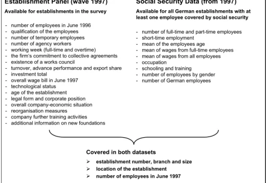
Figure 5.2: Included variables from the IAB Establishment Panel and the German Social Security Data.
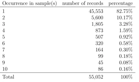
Table 5.2 displays how often different records occur in the synthetic samples.
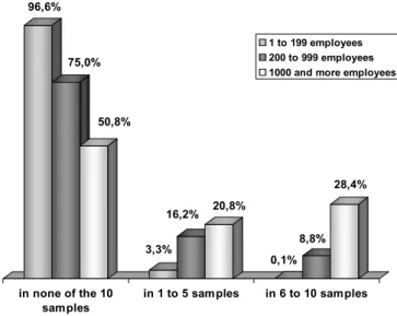
Figure 5.3: Occurrence of establishments already included in the original sur- sur-vey by establishment size.
+7

Referenzen

ÄHNLICHE DOKUMENTE

We compared the effects of both conditions on (1) performance measures, including bar-velocity and force output and; (2) psychological measures, including perceived autonomy,

We then introduce our imputation procedures for ordinary and overdispersed count data and present two evaluation studies: The first one generally tests our algorithms’ ability

This article both adds to some of these debates by arguing for the benefits of using informal and unstructured conversations in qualitative research, reiterating the critical

(2012), Items for a description of linguistic competence in the language of schooling necessary for learning/teaching mathematics (end of obliga- tory education) – An approach

local scale: The widespread use of term resilience in the national policy documents is not reflected on local level and is often at odds with the practical understanding

This extension of extrapolation is new: the idea of extending extrapolation to modular inequalities and Banach function spaces first appeared in [57] where the authors and

Imputing a single value for each missing datum and then analyzing the completed data using standard techniques designed for complete data will usually result in standard error

The priming chord creates a tonal reference frame (salience versus pitch of each tone sensation within the chord), and the test chord is perceived relative to that frame.. 5