in Soil Moisture and Terrestrial Water Storage from Multi-Sensor Earth Observations

(1)

Deutsche Geodätische Kommission der Bayerischen Akademie der Wissenschaften

Reihe C Dissertationen Heft Nr. 778

Sarah Abelen

Signals of Weather Extremes

in Soil Moisture and Terrestrial Water Storage from Multi-Sensor Earth Observations

and Hydrological Modelingmissions

München 2016

Verlag der Bayerischen Akademie der Wissenschaften in Kommission beim Verlag C. H. Beck

ISSN 0065-5325 ISBN 978-3-7696-5190-4

(2)

(3)

Deutsche Geodätische Kommission der Bayerischen Akademie der Wissenschaften

Reihe C Dissertationen Heft Nr. 778

Signals of Weather Extremes

in Soil Moisture and Terrestrial Water Storage from Multi-Sensor Earth Observations

and Hydrological Modelings

Vollständiger Abdruck

der von der Ingenieurfakultät Bau Geo Umwelt der Technischen Universität München zur Erlangung des akademischen Grades eines

Doktor-Ingenieurs (Dr.-Ing.) genehmigten Dissertation

von

Sarah Abelen

München 2016

Verlag der Bayerischen Akademie der Wissenschaften in Kommission beim Verlag C. H. Beck

ISSN 0065-5325 ISBN 978-3-7696-5190-4

(4)

Adresse der Deutschen Geodätischen Kommission:

Deutsche Geodätische Kommission

Alfons-Goppel-Straße 11 ! D – 80539 München

Telefon +49 – 89 – 230311113 ! Telefax +49 – 89 – 23031-1283 /-1100 e-mail post@dgk.badw.de ! http://www.dgk.badw.de

Prüfungskommission

Vorsitzender: Univ.-Prof. Dr.rer.nat. E. Rank Prüfer der Dissertation: 1. Univ.-Prof. Dr.-Ing. F. Seitz 2. Univ.-Prof. Dr.-Ing. U. Stilla 3. Univ.Prof. Dr.techn. W. Wagner,

Technische Universität Wien, Österreich

Die Dissertation wurde am 16.03.2016 bei der Technischen Universität München eingereicht und durch die Ingenieurfakultät Bau Geo Umwelt am 15.06.2016 angenommen.

.

Diese Dissertation ist auf dem Server der Deutschen Geodätischen Kommission unter <http://dgk.badw.de/>

sowie auf dem Server der Technischen Universität München unter

<https://mediatum.ub.tum.de/670323?show_id=1295206&style=full_text> elektronisch publiziert

die Veröffentlichung oder Teile daraus auf photomechanischem Wege (Photokopie, Mikrokopie) zu vervielfältigen.

ISSN 0065-5325 ISBN 978-3-7696-5190-4

(5)

5

Abstract

Soil moisture and terrestrial water storage (TWS) are of vital importance for water supply and agricultural production, and play a key role in the climate system. In this study interrelations between these two important hydrological parameters are analyzed. The analysis targets a better understanding of the dynamics of TWS, which in prior studies have primarily been related to changes in groundwater and surface water. Another objective is to gain insight about the drivers of soil moisture on global scale, and to find out whether the combined analysis of both parameters creates added value for their application in the field of natural disaster monitoring.

The global mapping of soil moisture and TWS is a relatively new field of research because operational satellite products, which provide information on both parameters on large scales, have just emerged in the past 15 years. This study makes use of TWS data from the satellite gravity mission GRACE (Gravity Recovery And Climate Experiment) and two surface soil moisture satellite products, which originate from the active microwave sensor ASCAT (Advanced SCATterometer) and the passive microwave sensor AMSR-E (Advanced Microwave Scanning Radiometer for Earth Observing System).

Additionally, global outputs for root zone soil moisture from the WGHM (WaterGAP Global Hydrology Model) and other ancillary data sets as for example for precipitation are integrated into the study.

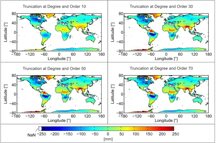
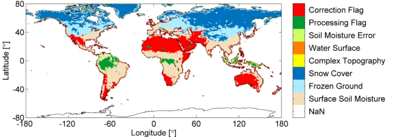
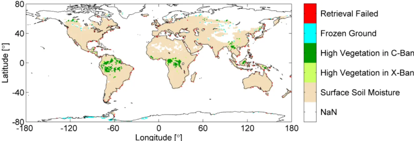
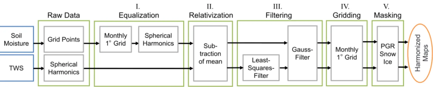
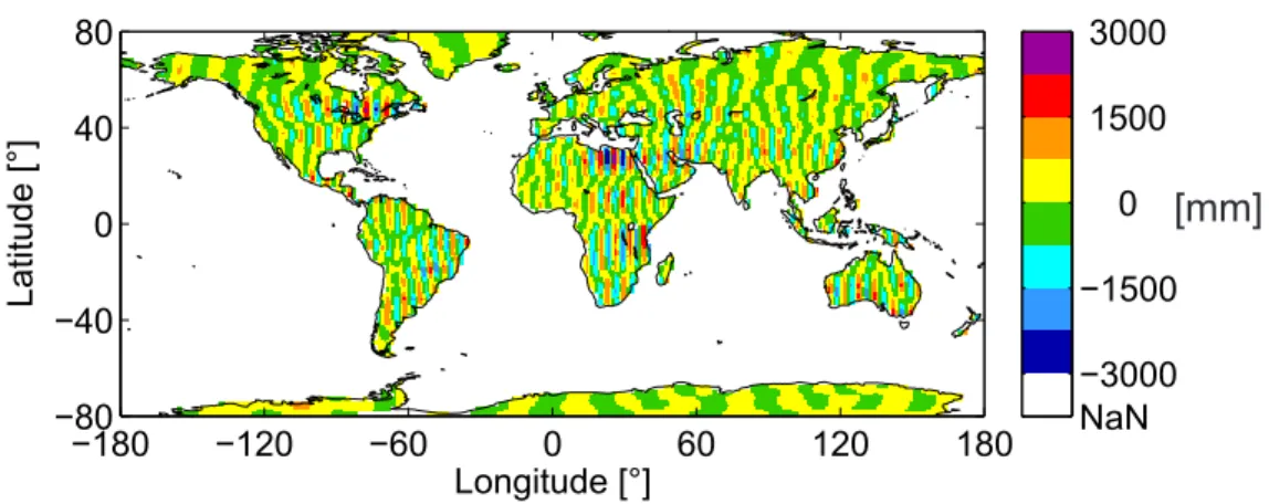
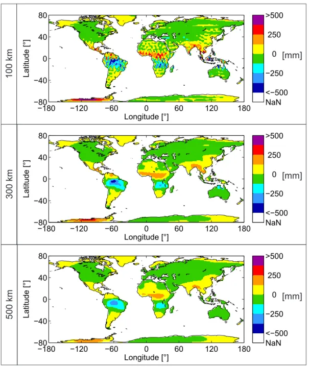
Following a three step approach first the question is posed whether it is at all feasible to relate data sets for soil moisture and TWS because especially GRACE data differ significantly in data structure and processing from the global soil moisture products. In order to achieve comparable formats, all data sets are harmoniously processed. Main steps include the conversion into spherical harmonics, Gauss filtering and the projection of all data onto a 1^◦×1^◦ grid in monthly time intervals. A least-squares filter is additionally applied to the GRACE data. Results show that the main impact of the harmonious processing is homogeneous spatial smoothing of the data in most parts of the world. Exceptions are mainly deserts. In these regions variations in soil moisture are artificially amplified and altered through the conversion into spherical harmonics and spatial leakage from Gauss filtering. Therefore, these areas are excluded from the analyses. Furthermore, regions of low data quality are identified individually for each data set via correlation and time shift analysis. The information on the data quality is also integrated in the analysis.

Second, interrelations between soil moisture and TWS; and soil moisture and other water storage components are analyzed. Therefore, each hydrological signal is split into a seasonal signal and its anomaly. Both parts of the signal are then correlated separately and in sum for different pairs of water storage components. Furthermore, time shifts between different hydrological parameters are calculated. The analysis shows that the seasonal signal of soil moisture dominates the seasonal signal of other storage components over large areas, especially in the southern hemisphere. However, in some of these areas the seasonal amplitude of soil moisture is very low (<40 mm). In regions where soil moisture and TWS are in high agreement (e.g., southern China and India), variations in soil moisture are strongly related to those of other dominating storage components such as groundwater or surface water. A special case is the Sahel zone. In this region variations of soil moisture correlate strongly with changes in TWS (>=0.6), because the seasonal signal of soil moisture is dominant and has a large

(6)

6 Abstract

amplitude (ranging between 40 and 140 mm according to WGHM). Therefore, soil moisture plays a key role for TWS in the Sahel zone.

Third, variations in soil moisture and TWS are compared to gain insight into weather extremes in the La Plata Basin in South America. Specifically those events are brought into focus that had a severe impact on society, and therefore have been registered as natural disasters in the International Disaster Database EM-DAT. Results show that in the La Plata Basin extreme weather events accumulate in El Niño and La Niña years. While most variations in soil moisture can be assigned to single natural disasters, changes in TWS mainly correspond to spatially extended and long-duration drought and flood periods. For two events, namely the La Plata drought of 2009 and the flooding period during the El Niño event in the boreal winter of 2009/2010, changes in soil moisture serve as indicator for upcoming lack or surplus in TWS. Although there is generally a high correspondence between natural disasters and weather extremes, there are also some discrepancies between both data sets. For example, Bolivia was only moderately hit by the 2009 La Plata drought but still more than one hundred thousand people were affected. In contrast the southeastern part of the basin was struck at a similar level but no social impacts have been registered for this region. A possible reason for this discrepancy is the fact that the destructiveness of a disaster does not only depend on the severity of the weather extreme but also on social factors such as population density and the preparedness of the population. Furthermore, information provided within EM-DAT might be incomplete or faulty as the collection of these critical data is challenging on an international level.

In summary this study showed that soil moisture and TWS are interrelated over large parts of the world, either because soil moisture contributes significantly to seasonal changes in TWS or because soil moisture changes proportionally with other dominant storage components. In the La Plata Basin this information could be used for the analysis of extreme weather events and associated natural disasters, which had a high impact on society. By the integration of additional information on the absolute amount of soil moisture in the entire root zone, future studies could investigate the concrete share of soil moisture in TWS.

(7)

7

Zusammenfassung

Sowohl der terrestrische Wasserspeicher als auch die Bodenfeuchtigkeit sind für die Wasserversorgung und die landwirtschaftliche Produktion von lebenswichtiger Bedeutung und haben Schlüsselfunktionen im Klimasystem der Erde. In dieser Studie wird untersucht welche Wechselwirkungen und Zusam- menhänge zwischen diesen beiden wichtigen hydrologischen Parametern bestehen. Ziel der Analyse ist es ein besseres Verständnis über die Veränderungen des terrestrischen Wasserspeichers zu erlangen, die bislang meistens auf Variationen des Grundwassers und der Oberflächengewässer zurückgeführt wurden.

Außerdem sollen die Ergebnisse Aufschluss darüber geben, welche Faktoren die Bodenfeuchtigkeit auf globaler Ebene beeinflussen, und ob die Verknüpfung beider Parameter einen Mehrwert für ihre Verwendung beim Monitoring von Naturkatastrophen darstellt.

Die globale Beobachtung der Bodenfeuchtigkeit und des terrestrischen Wasserspeichers ist ein relativ neues Forschungsfeld, da Satellitendaten, die globale Informationen über beide Parameter liefern, erst seit ca. 15 Jahren operationell verfügbar sind. Diese Studie basiert auf Daten der Gravitations- feldmission GRACE (Gravity Recovery And Climate Experiment), die unter anderem Veränderungen des terrestrischen Wasserspeichers wiederspiegeln, und auf den Daten zweier Satellitenmissionen zum Beobachten der Oberflächenfeuchtigkeit: dem aktiven Mikrowellensensor ASCAT (Advanced SCAT- terometer) und dem passiven Mikrowellensensor AMSR-E (Advanced Microwave Scanning Radiometer for Earth Observing System). Diese Daten werden ergänzt durch die globalen Bodenfeuchtigkeitswerte des hydrologischen Modells WGHM (WaterGAP Global Hydrology Model) in der Wurzelzone und durch zusätzliche Datensätze zum Beispiel über den Niederschlag.

Diese Studie ist in drei Teile gegliedert. Als erster Schritt geht sie der Frage nach, ob es überhaupt möglich ist Datensätze über Bodenfeuchtigkeit und den terrestrischen Wasserspeicher in Verbindung zu bringen, da insbesondere GRACE-Daten sich erheblich in ihrer Struktur und Prozessierung von den globalen Bodenfeuchtigkeitsdaten unterscheiden. Um die Formate der verschiedenen Datensätze aneinander anzugleichen, wird die Prozessierung aller Datensätze vereinheitlicht. Dies beinhaltet, dass alle Daten zunächst in Kugelflächenfunktionen dargestellt werden und mit einem Gauß-Filter geglättet werden. Dann werden die monatlichen Mittelwerte wieder auf ein 1^◦ × 1^◦ Gitter projiziert. Die GRACE-Daten werden zusätzlich mit einem Kleinste-Quadrat-Filter geglättet. Die Ergebnisse zeigen, dass die vereinheitlichte Prozessierung in den meisten Gebieten der Erde vor allem eine gleichförmige räumliche Glättung zur Folge hat. Ausnahmen sind vor allem Wüstengebiete. In diesen Regionen werden aufgrund der Umrechnung in Kugelflächenfunktionen und aufgrund von scheinbaren räumlichen Verlagerungen, die unter Anwendung des Gauß-Filters entstehen, Veränderungen der Bodenfeuchtigkeit verstärkt und abgewandelt. Deshalb werden diese Gebiete in den folgenden Analysen nicht berück- sichtigt. Zusätzlich wird die Qualität aller Datensätze durch die Berechnung von Korrelationskoeffi- zienten und zeitlichen Verschiebungen zwischen den Datensätzen überprüft. Auch die Ergebnisse zur Datenqualität werden in den weiteren Analysen berücksichtigt.

Als zweiter Schritt werden hydrologische Zusammenhänge zwischen der Bodenfeuchtigkeit und dem terrestrischen Wasserspeicher sowie zwischen der Bodenfeuchtigkeit und anderen Wasserspeichern analysiert. Hierfür wird jedes hydrologische Signal in eine saisonale Komponente und dessen Abwei- chung aufgeteilt. Anschließend werden beide Komponenten separat und in der Summe für verschie-

(8)

8 Zusammenfassung

dene Wasserspeicherkombinationen korreliert. Außerdem werden zeitliche Verschiebungen zwischen verschiedenen hydrologischen Parametern ermittelt. Die Analyse zeigt, dass das saisonale Signal der Bodenfeuchtigkeit insbesondere in weiten Teilen der südlichen Hemisphäre das saisonale Signal anderer Wasserspeicher dominiert. Allerdings ist die Amplitude des saisonalen Signals in einigen dieser Regionen sehr gering (<40 mm). In Gebieten, in denen die Variationen der Bodenfeuchtigkeit mit denen des terrestrischen Wasserspeichers übereinstimmen (wie zum Beispiel in Süd-China und Indien), sind Varia- tionen der Bodenfeuchtigkeit an die der anderen dominierenden Wasserspeicher, wie Grundwasser oder Oberflächenwasser, gekoppelt. Eine Ausnahme ist die Sahel-Zone. In dieser Region gibt es höhere Korrelationswerte (>=0.6) zwischen den Veränderungen der Bodenfeuchtigkeit und des terrestrischen Wasserspeichers, weil das saisonale Signal der Bodenfeuchtigkeit dominant ist und eine hohe Ampli- tude (variierend zwischen 40 und 140 mm basierend auf dem WGHM) aufweist. Dies bedeutet, dass die Bodenfeuchtigkeit in der Sahel-Zone eine Schlüsselfunktion für den terrestrischen Wasserspeicher einnimmt.

Als dritter Schritt werden Variationen der Bodenfeuchtigkeit und des terrestrischen Wasserspeichers verglichen, um Aufschluss über Extremwetterereignisse im La Plata Einzugsgebiet in Südamerika zu erlangen. Dabei stehen insbesondere Ereignisse im Vordergrund, die schwerwiegende Auswirkungen auf die Gesellschaft hatten und deshalb als Naturkatastrophen in die internationale Katastrophendatenbank EM-DAT aufgenommen wurden. Die Ergebnisse zeigen, dass im La Plata Einzugsgebiet Extremwet- terereignisse mit El Niño und La Niña Jahren zusammenfallen. Während Veränderungen der Boden- feuchtigkeit zum größten Teil einzelnen Naturkatastrophen zugeordnet werden können, zeigen Varia- tionen des kontinentalen Wasserspeichers Übereinstimmung mit länger anhaltenden Hochwasser- und Trockenperioden. Bei zwei Ereignissen, nämlich der La Plata Dürre 2009 und der Überschwemmungs- periode während des El Niño Winters 2009/2010, weisen Veränderungen der Bodenfeuchtigkeit auf eine folgende Knappheit oder einen Überschuss im terrestrischen Wasserspeicher hin. Obwohl Naturkata- strophen und Wetterextrema weitestgehend übereinstimmen, gibt es auch Unstimmigkeiten zwischen beiden Datensätzen. Zum Beispiel war die La Plata Dürre in Bolivien von moderater Stärke und mehr als einhunderttausend Menschen waren von der Dürre betroffen. Der südöstliche Teil des Einzugsgebiets wurde hingegen in vergleichbarer Stärke von der Dürre getroffen, aber in dieser Region gab es keine Einträge über soziale Auswirkungen. Ein möglicher Grund für diese Unstimmigkeit ist die Tatsache, dass die Zerstörungskraft eines Ereignisses nicht nur von der Schwere des Wetterextrems abhängt sondern auch von sozialen Faktoren wie der Bevölkerungsdichte und der Katastrophenvor- sorge. Außerdem ist es auch möglich, dass die Informationen der Datenbank EM-DAT unvollständig oder fehlerhaft sind, da das Sammeln dieser kritischen Daten auf internationaler Ebene eine Heraus- forderung darstellt.

Zusammengefasst hat diese Studie gezeigt, dass die Bodenfeuchtigkeit und der terrestrische Wasser- speicher in weiten Teilen der Erde im Zusammenhang stehen, weil entweder die Bodenfeuchtigkeit die saisonale Veränderung des terrestrischen Wasserspeichers signifikant beeinflusst oder weil sich die Bodenfeuchtigkeit zeitgleich mit anderen dominanten Wasserspeichern verändert. Im La Plata Einzugsgebiet konnten diese Informationen für die Analyse von Extremwetterereignissen und den damit verbundenen Naturkatastrophen, die schwerwiegende Auswirkungen auf die Gesellschaft hatten, genutzt werden. Durch die Einbindung von weiteren Informationen über den Absolutbetrag der Boden- feuchtigkeit in der Wurzelzone, könnte in zukünftigen Studien der exakte Anteil der Bodenfeuchtigkeit am kontinentalen Wasserspeicher berechnet werden.

(9)

9

Preface

In this PhD thesis the results of three peer-reviewed publications are integrated. Those publications are listed in the following:

Abelen S, Seitz F, Schmidt M, G¨untner A (2011) Analysis of regional variations in soil moisture by means of remote sensing, satellite gravimetry and hydrological modelling. In: GRACE, Remote Sensing and Ground-Based Methods in Multi-Scale Hydrology, IAHS Red Book Series, Nr. 343, International Association of Hydrological Sciences, pp 9–15

Abelen S, Seitz F (2013) Relating satellite gravimetry data to global soil moisture products via data harmonization and correlation analysis. Remote Sensing of Environment 136:89–98, DOI 10.1016/j.rse.2013.04.012

Abelen S, Seitz F, Abarca-del Rio R, G¨untner A (2015) Droughts and Floods in the La Plata Basin in Soil Moisture Data and GRACE. Remote Sensing 7(6):7324–7349, DOI 10.3390/rs70607324 Whenever a passage of one of those publications is used in this thesis it is marked as following:

⊳ ... ⊲ (Abelen et al, 2011)

⊳ ... ⊲ (Abelen and Seitz, 2013)

⊳ ... ⊲ (Abelen et al, 2015)

This marking does not mean that the text is copied word by word. The highlighted passage might contain slight modifications, which do not alter the content and meaning of the text. For example more recent publications might be added to the references, phrases like “we used the method”, might be rephrased to “the method was used”, references to previous chapters might be added, or explanatory notes might be provided.

(10)

(11)

11

Abbreviations

AMSR-E Advanced Microwave Scanning Radiometer for Earth Observing System ASCAT Advanced SCATterometer

CSR Center for Space Research at University of Texas at Austin DLR German Aerospace Center

ECMWF European Centre for Medium-Range Weather Forecasts

EGSIEM European Gravity Service for Improved Emergency Management EM-DAT The International Disaster Database

EOF Empirical Orthogonal Function EPOS Earth Parameter and Orbit System GFZ German Research Centre for Geosciences GPCC Global Precipitation Climatology Center GRACE Gravity Recovery And Climate Experiment

GW Groundwater

ISMIN International Soil Moisture Network JPL Jet Propulsion Laboratory

LEO Low Earth Orbit LPB La Plata Basin LSM Land-Surface Model

MIRAS Microwave Imaging Radiometer using Aperture Synthesis NASA National Aeronautics and Space Administration

NOAA National Oceanic and Atmospheric Administration NRCS Natural Resource Conservation Service

ONI Oceanic Ni˜no Index PC Principal Component

PCA Principal Component Analysis PGR Post-Glacial Rebound

RQ Research Question

(14)

14 Abbreviations

SAR Synthetic Aperture Radar SGG Satellite Gravity Gradiometry SH Spherical Harmonics

SMAP Soil Moisture Active Passive

SMN Argentinean National Meteorological Service SMOS Soil Moisture and Ocean Salinity

SST Satellite-to-Satellite Tracking

SST-hl high-low Satellite-to-Satellite Tracking SST-ll low-low Satellite-to-Satellite Tracking SUR Surface Water

SWI Soil Water Index

TRMM Tropical Rainfall Measuring Mission TUM Technische Universit¨at M¨unchen TWS Terrestrial Water Storage

UNISDR United Nations Office for Disaster Risk Reduction UNEP United Nations Environmental Programme

USDA United States Department of Agriculture USGS United States Geological Survey

WaterGAP WaterGlobal Assessment and Prognosis WGHM WaterGAP Global Hydrology Model

(15)

15

1 Introduction

1.1 Motivation

The Food and Agricultural Organization declared the year 2015 as the International Year of Soils. Soil moisture plays a crucial role in food security and is a key variable in the climate system (Section 2.1).

It is a storage component for precipitation and a source of water for the atmosphere by influencing plant transpiration and bare soil evaporation (Seneviratne et al, 2010). In 2009 soil moisture has been recognized as an Essential Climate Variable within the Intergovernmental Panel on Climate Change and the United Nations Framework Convention on Climate Change. Terrestrial water storage (TWS) refers to all water which is stored over the continents (Section 3.1). It is an important part of the hydrological cycle as it entails the fraction of precipitation, which reaches the Earth’s surface and is neither evaporated nor drained through runoff to the ocean (Schmidt et al, 2006c).

⊳ Soil moisture and TWS are closely linked, as soil moisture is an essential component of TWS in addition to surface water, snow, ice, and groundwater. Furthermore, both parameters strongly depend on the difference between inflow (precipitation) and outflow (percolation, drainage, and evapotranspiration) of the soil and its water-holding capacity (as a function of, e.g., soil physical properties). ⊲ (Abelen et al, 2015)

In the past both parameters, TWS and soil moisture, were not mapped over extensive areas, because adequate large-scale monitoring systems (referring to spatial extents>100²km², herein as defined by Ochsner et al, 2013) were not operationally available (see Section 2.1 and Section 3.1). This changed significantly in the last 15 years. In 2003 the satellite gravity mission GRACE (Gravity Recovery And Climate Experiment) was launched enabling for the first time in history the global mapping of changes in TWS. From 2002 onwards the operational availability of global soil moisture products was made possible with the launch of at least five major satellite missions (AMSR-E, ASCAT, SMOS, SMAP and Sentinel-1).

Recent data sets from satellites (see Section 2.2 and Section 3.2), in combination with outputs of global hydrological models (see Section 2.3 and Section 3.3), have opened up new possibilities for the analysis of soil moisture and TWS on global scale. At the same time there is a growing need for hydrological and climatological studies because of increasing pressure on agriculture due to population growth, and changing weather and climate (Overgaard et al, 2005), which is coupled with more intense and frequent weather extremes.

The validation and application of those newly available data sets has caught the interest of many scientists (see Section 2.4 and Section 2.5 for soil moisture and Section 3.4 and Section 3.5 for TWS).

Key challenges which still remain have been described as the following:

“Two main issues with GRACE estimates are, however:

1. the necessary disaggregation of the data in separate estimates of the individual terrestrial water storage components (e.g. soil moisture, groundwater, snow);

(16)

16 1 Introduction

2. the still coarse resolution of the estimates” (Seneviratne et al, 2010)

“In closing, we again note the growing need to develop the science necessary to make effective use of the rising number of large-scale soil moisture data sets.” (Ochsner et al, 2013)

Previous studies have analyzed large-scale soil moisture and TWS products individually or in combination with other data sets (e.g., on precipitation, river runoff). However, studies which primarily connect global soil moisture data sets with TWS estimates from GRACE were lacking. The focus of this thesis is on the combined analysis of recent large-scale soil moisture and TWS products to address the above mentioned open challenges (more detailed information on the contribution of this study is given in Section 2.6 and Section 3.6). The motivation is to find out which role soil moisture plays within TWS and how the dynamics of soil moisture and TWS are linked on global scale. A further objective is to find out if the combination of both data sets adds value to their application in the field of natural disaster monitoring.

1.2 Target of Research

The main target of this research is to give answer to the question whether it is feasible to compare large-scale soil moisture products with TWS from GRACE to tackle the above mentioned challenges and those which are listed in more detail in Section 2.6 and Section 3.6. More specifically this thesis addresses three main research questions (RQ 1 to RQ 3):

1. Is it feasible to compare the various soil moisture products with TWS from GRACE with respect to the different characteristics of the data sets, considering in specific:

a) Their varying data structures (e.g. in terms of spatial and temporal resolution and required preprocessing), and

b) Their heterogeneous data quality?

2. Which hydrological interdependencies exist between soil moisture and TWS, considering in specific:

a) The relative share of soil moisture in the seasonal signal of TWS,

b) Correlations and time shifts between variations in soil moisture and TWS,

c) Interdependencies between soil moisture and other hydrological parameters such as groundwater and surface water?

3. What can we learn with the help of soil moisture and TWS from GRACE about hydrological extremes and associated natural disasters?

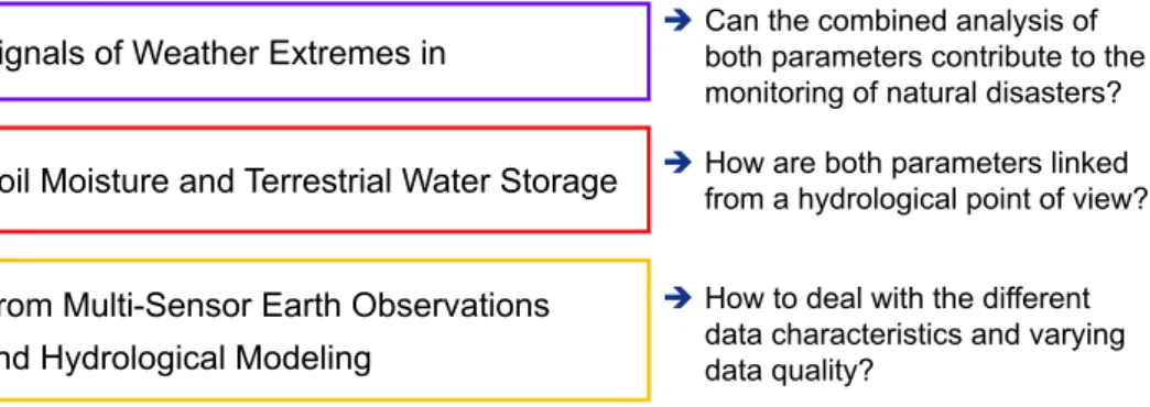
This three step approach is also reflected in the title of this thesis as shown in Figure 1.1. First, this study focusses on data-related issues as multi-sensor Earth observations and outputs of one hydrological model have to be brought into comparable formats. This establishes the basis for the following investigations. Second, the two hydrological variables, soil moisture and TWS, and their interrelations are brought into focus. It is investigated in which parts of the world variations of both data sets are in agreement and why hydrologic interrelations exist. Third, it is analyzed exemplarily for the La Plata Basin in South America if the knowledge on links between soil moisture and TWS can be used for the monitoring of weather extremes, which have high impact on society.

(17)

1.3 Structure of the Dissertation 17

Figure 1.1: Title of the thesis and the followed three step approach.

1.3 Structure of the Dissertation

The structure of the thesis is shown in Figure 1.2. This introduction is followed by a state of the art on the large-scale mapping of soil moisture (Chapter 2) and the large-scale mapping of TWS (Chapter 3). After an introduction to the hydrological parameters soil moisture (Section 2.1) and TWS (Section 3.1), recent large-scale mapping techniques by satellites and models are described (see Section 2.2 and Section 2.3 for soil moisture, and Section 3.2 and Section 3.3 for TWS, respectively).

Furthermore, an overview is given on studies which were dedicated to the validation and application of those data sets (see Section 2.4 and Section 2.5 for soil moisture, and Section 3.4 and Section 3.5 for TWS, respectively). At the end of both state of the art chapters the contribution of this study is described in detail (see Section 2.6 for soil moisture, and Section 3.6 for TWS).

Next, the various data sets used in this study are described (Chapter 4). They include two surface soil moisture products from the satellite sensors ASCAT and AMSR-E (see Section 4.1 and Section 4.2, respectively), information on TWS variation from the satellite mission GRACE (Section 4.3), and outputs for various storage components, which sum up to TWS (including root zone soil moisture), from WGHM (Section 4.4). Further ancillary data sets comprise precipitation data from GPCC (Section 4.5), information on El Niño and La Niña years based on the Oceanic Niño Index (Section 4.6), and a list of natural disasters provided by the International Disaster Database EM-DAT (Section 4.7).

Chapter 5 describes the methods which are used to align the formats of all data sets and to compare them in spatial and temporal terms. First, interrelations between variations in soil moisture and variations in TWS from GRACE are theoretically discussed and several assumptions for the following analysis are formulated (Section 5.1). Afterwards the approach for harmonizing soil moisture data and data from satellite gravimetry is described (Section 5.2). The harmonious processing is particularly adjusted to the special characteristics of GRACE data, which is why the data sets are introduced previous to the method, herein. As satellites only provide information on the surface soil moisture, they are scaled with respect to the root zone soil moisture which is provided by WGHM (Section 5.3).

Interrelations among the data sets are calculated via correlation (Section 5.4), time shift (Section 5.5), and principal component analysis (Section 5.6). As last step hydrological extremes in soil moisture and TWS are linked to natural disasters, which had destructive impact on society (Section 5.7).

Results, which concern the comparability of data sets, are presented in Chapter 6. They reflect the impact of the harmonious data processing (Section 6.1) and provide spatial information on the data quality of the global soil moisture and TWS products (see Section 6.2 and Section 6.3, respectively).

The results of Chapter 6 provide the basis for the analysis of hydrological interrelations. They are summarized in terms of RQ 1a and 1b in the last section of this chapter (Section 6.4).

(18)

18 1 Introduction

Chapter 7 shows results, which emphasize how soil moisture and TWS are linked over large areas.

The results provide information about the seasonal amplitude of soil moisture and how it relates to the seasonal amplitudes of other storage components (see Section 7.1). Furthermore, they show in which regions of the world soil moisture and TWS are strongly interconnected (Section 7.2) and how these findings are related to interdependencies between soil moisture and other storage components (Section 7.3). In the final summary of this chapter RQ 2a, 2b, and 2c are addressed (Section 7.4).

The focus of Chapter 8 is on the application of soil moisture and TWS data for the monitoring of hydrological extremes in the La Plata Basin in South America (Section 8.1). Therefore, the quality of the used soil moisture data (Section 8.2) and the interdependency of soil moisture and TWS (Section 8.3) are analyzed more in detail for this region. Then, time series of soil moisture and TWS data are matched with impacts of weather extremes, which have been registered within the International Disaster Database EM-DAT (Section 8.4). Also connections to El Ni˜no and La Ni˜na years are emphasized. The summary of this chapter is devoted to RQ 3 (Section 8.5).

In Chapter 9 final conclusions from all findings of this thesis (which are summarized in Section 6.4, Section 7.4, and Section 8.5) are drawn with respect to the comparability of the used data sets, interrelations of soil moisture and TWS on global scale, and potential benefits of integrating both data sets into the analysis of weather extremes. The outlook in Chapter 10 describes new potential approaches to gain deeper insight about interdependencies between soil moisture and TWS on large scale.

(19)

1.3 Structure of the Dissertation 19

Figure 1.2: Structure of the thesis.

(20)

(21)

21

2 Large-Scale Mapping of Soil Moisture

2.1 Introduction to Soil Moisture

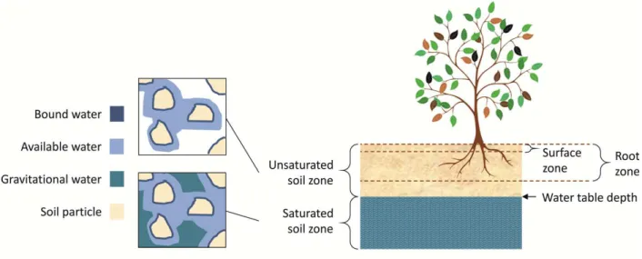
Soil moisture is usually defined as the water contained in the unsaturated soil zone at the surface of the Earth (Petropoulos, 2014; Hillel, 1998). In the unsaturated and saturated soil zone one distinguishes between three main types of water (Figure 2.1). The water which is surrounding the soil in the first molecular layers is strongly held by the soil matrix. It is unavailable to plants and also called bound water (Wagner, 1998).The highest possible amount of bound water is defined by the so called permanent wilting point. Also inaccessible to plants is gravitational water. Gravitational water cannot be held by the soil matrix against gravitational forces and drains to the saturated soil zone. It is formed above the so called field capacity (Seneviratne et al, 2010).

Water accessible to plants in the unsaturated soil zone is neither tightly bound to the soil water (as in the case of bound water) nor subject to gravitational drainage (as in the case of gravitational water) (Seneviratne et al, 2010; Hillel, 1998). Its lower limit is defined by the permanent wilting point and its upper limit is defined by the field capacity. The field capacity and the permanent wilting point (and with it also the amount of bound, available and gravitational water) vary geographically as they depend on the properties of the soil (e.g. the texture of the soil). The permanent wilting point (and with it also the amount of bound water) additionally depends on the vegetation type (Seneviratne et al, 2010; Sperry et al, 2002).

Figure 2.1: Schematic on the presence of bound, available and gravitational water in the unsaturated and saturated soil zone (left), and the location of the surface zone (as captured by microwave satellite remote sensing) and the root zone (being specifically relevant to agro-ecological studies) in the unsaturated soil zone (right).

(22)

22 2 Large-Scale Mapping of Soil Moisture

The targeted fraction of soil moisture which is measured or estimated differs significantly among various techniques (Dorigo et al, 2010). Microwaves sensors on satellite platforms capture the moisture in the surface zone of the soil (Figure 2.1, right). For bare soil this zone is approximately up to 2 cm deep (Escorihuela et al, 2010; Schneeberger et al, 2004), mainly depending on the operating wavelength of the satellite sensor and the soil moisture content (see Section 2.2). For models the depth of the considered soil zone is usually deeper. Depending on the model the moisture of one or more discrete soil layers are simulated (see Section 3.3).

Often the targeted fraction of the soil is the root zone (Figure 2.1, right) because the available water in this zone is of specific interest to the agricultural sector (Wang et al, 2007) and a key parameter for investigations of soil moisture-climate interactions (Seneviratne et al, 2010). As the rooting depth of vegetation (defining the root zone) and the water table depth (defining the unsaturated soil zone) vary over space and time, the targeted soil fraction may not be constant but change as function of space and time. When comparing different soil moisture products possible differences in the observed fraction of soil moisture (e.g. surface soil moisture vs. root zone soil moisture) have to be taken into account (Dorigo et al, 2010).

Soil moisture is vertically (at different soil depth) and horizontally (at different locations) heteroge- neously distributed and shows strong fluctuation over time (e.g. at the soil surface within hours). This large variability is on the one hand based on geographic factors such as varying soil types and topography. On the other hand it is driven by manifold complex processes, such as soil moisture-precipitation coupling, soil moisture-temperature coupling and soil moisture-evapotranspiration coupling (Senevi- ratne et al, 2010).

When analyzing variations of soil moisture at different scales two main components can be distin- guished. The first small-scale component (acting in the range of centimeters to hundreds of meters) refers to changes in soil moisture which originate from the heterogeneity in vegetation, soil type and topography. The second large-scale component (acting in the range of hundreds of kilometers) includes variability in soil moisture which is induced by large patterns of precipitation and evapotranspiration, resulting from meteorological and climate events (Scipal et al, 2005).

Comprehensive and continuous measurements of soil moisture from in-situ or proximal sensing techniques are currently not available on large scales, as existing networks are worldwide unevenly distributed. Especially in dry areas, at high latitudes, and in the tropics the number of stations is limited (Ochsner et al, 2013). Recently, efforts have been made to establish large in-situ networks with spatial extends >100²km². A list of large scale in-situ soil moisture monitoring networks is provided by Ochsner et al (2013).

Furthermore, the International Soil Moisture Network (ISMIN; https://ismn.geo.tuwien.ac.at/) has been founded in 2009 (Dorigo et al, 2011a,b). It is a joint initiative from the Global Energy and Water Cycle Experiment, the Group of Earth Observations and the Committee on Earth Observations Satellites, funded by the European Space Agency. ISMIN harmonizes and collects in-situ soil moisture data from different networks and makes them accessible through a centralized data portal. Many data from operational soil moisture networks are downloaded automatically and are available in near real time. Those data are essential for sensor calibration and the validation of soil moisture products from remote sensing (Ochsner et al, 2013, see Section 2.4).

(23)

2.2 Soil Moisture from Microwave Remote Sensing 23

2.2 Soil Moisture from Microwave Remote Sensing

Remote sensing techniques, estimating soil moisture indirectly from tower, aircraft or satellite platforms, have been used since the early 1960s (Ulaby and Long, 2014). The history and technological development of those measurements (and also of in-situ measurements) are described in detail by Ochsner et al (2013) and Ulaby and Long (2014). The use of satellite platforms for the remote sensing of soil moisture made the consistent and frequent global mapping of soil moisture possible (Kumar and Reshmidevi, 2013). Specifically microwave sensors with wavelength from 1 m to 1 mm (corresponding to frequencies of 0.3 to 300 GHz respectively) are suitable to provide quantitative measurements of soil moisture. Most important bands are X-band (wavelength = 2.5-3.8 cm, frequency = 12-8 GHz ), C-band (wavelength 3.8-7.6, frequencies 8-4 GHz), and L-band (wavelength = 15-30 cm, frequency

= 2-1 GHz).

Unfortunately all bands may be affected by radio frequency interference (RFI). This is also true for in principle protected bands, which are reserved for passive sensors only such as the L-band (Wagner et al, 2007). Impacts on the satellite signal through cloud coverage, rain, and vegetation decrease with increasing wavelength. For wavelengths larger than 4 cm cloud coverage and rain are negligible.

With increasing wavelength the signal penetrates more deeply into the soil, whereby the penetration depth additionally depends on the dielectric properties of the ground and is deeper for surfaces with low vegetation cover and low soil moisture (Ulaby and Long, 2014).

Microwave sensors are able to sense soil moisture as they are sensitive to the dielectric constant of the ground, which increases with increasing amount of water in the soil (Ulaby et al, 1982). The real part of the dielectric constant determines the propagation characteristics of the signal through the soil, while the imaginary part determines the energy losses (de Jeu et al, 2008). Dielectric properties of common materials at the Earth’s surface are provided in Table 2.1 as summary of the dielectric values presented by Wagner (1998). The table shows the large differences in the dielectric properties of dry soil and water. For example, the real part of the dielectric constant has a value of about 3 for dry soil and a value of about 70 and for water (Jackson, 2005). Furthermore, the table highlights that the dielectric constants of liquid and frozen water as well as of bound and free (available and gravitational) water differ significantly. The dielectric constant of vegetation increases with increasing moisture content. Challenges for soil moisture retrieval which arise from the mixture of different dielectric properties of various materials on the ground are highlighted in Table 2.3 in Section 2.4.

Table 2.1: Dielectric properties at C-band of common materials at the Earth’s surface, summarized from Wagner (1998).

(24)

The link between the dielectric constant and the sensed microwave signal at the satellite is given by the reflectivity of the ground, expressed by the Fresnel reflection equation:

r_{surf fp} =

cosθ−p

k−sin²θ cosθ+p

k−sin²θ

2

. (2.1)

The Fresnel reflection equation tells that the reflectivity of the surface (rsurf) for a certain frequency band (f), and polarization (p), depends on the viewing angle of the sensor (θ) and the dielectric constant (k) of the ground. This simplified equation can be applied, assuming that the Earth has a plane surface and that the interface between the surface soil layer and the air (approximated as vacuum) have uniform dielectric properties (Jackson, 2005).

For the remote sensing of soil moisture two main techniques exist: active and passive microwave remote sensing. Passive sensors (radiometers) measure the natural thermal radio emission from the Earth, which is expressed as brightness temperature (TB) for a particular frequency band (f), and polarization (p) (Njoku and Li, 1999):

T_{B f p}=e_{surf fp}Tsurfe⁻^τ^f +Tup+

1−e_{surf fp}

Tdowne⁻^τ^f +

1−e_{surf fp}

Tspacee⁻²^τ^f. (2.2) The brightness temperature is provided in degree Celsius or Kelvin and refers to the temperature a black body (for which emissivity = absorptivity = 1) would be in order to emit the recorded radiance at a given frequency and polarization (Liang et al, 2012).

The first term on the left side of the equation accounts for the emitted radiation from the surface. It is the product of the emissivity of the surface (e_{surf fp}), the physical temperature of the surface (Tsurf) and the attenuation of the radiation by the atmospheric opacity (τf), also referred to as optical depth. The second term (Tup) is atmospheric upwelling radiation. The third term is the atmospheric downwelling radiation (Tdown), which has been reflected at the surface (1−e_{surf fp} = r_{surf fp}) and is also attenuated by the atmosphere. The last term accounts for the cosmic background radiation (Tspaceis the cosmic background temperature), which has been travelling twice through the atmosphere (once by reaching the surface and once after reflection at the surface). Taking into account that the reflectivity is equal to one minus the emissivity (Kirchhoff’s law; Schanda, 1986) the formula can be directly linked to the reflectivity of the surface, which is again linked to the dielectric constant of the ground (see Equation 2.1).

Equation 2.2 highlights the main components influencing the brightness temperature which is measured by the satellite. The last term on the cosmic background radiation is about 2.7 K (Ulaby et al, 1982) and the upwelling and downwelling atmospheric radiation can be expressed as products of the weighted average atmospheric temperature and the atmospheric emissivity (Bevis et al, 1992). There- fore, the main remaining term in the equation is the first one, which mainly depends on the emissivity and temperature of the surface.

The physical temperature of the Earth can be estimated through model predictions, satellite measurements or air temperature observations, whereby the quality of those estimates is crucial for the quality of the soil moisture products (Parinussa et al, 2011). With information on the land surface temperature, the emissivity of the ground and with it also the dielectric constant and finally the soil moisture can be computed from the brightness temperature measured at the satellite. The emissivity of the ground and with it also the brightness temperature decreases with increasing soil moisture.

(25)

The second remote sensing technique for the measurement of soil moisture is based on active sensors, which are also called radars (radio detection and ranging). Those send an energy pulse actively to the Earth and measure the energy which is scattered back from the Earth’s surface to the sensor. The received power at the satellite of a transmitted signal, which has been scattered back to the sensor by one specific target, has been described by Ulaby et al (1982) with the widely used monostatic (radar transmitter and receiver are co-located) radar equation (Joseph, 2005; Rees, 2013; Wagner, 1998):

Pr = PtG 4πR² σ 1

4πR² λ²G

4π = λ² (4π)³

PtG²

R⁴ σ, (2.3)

where:

Pr received power Pt transmitted power G gain of the antenna

λ wavelength of the radar signal

R distance (range) between radar and target σ radar cross-section of the target

The equation tells that the received Power (Pr) is equal to the power density that the transmitter produces at the target (first term on right hand side of the equation), times the radar cross-section of the target (second term on right hand side of the equation), times the isotropic spread of the intercepted power from the target back to the radar (third term on right hand side of the equation), times the effective area of the antenna that collects the returning power density (fourth term on right hand side of the equation). All parameters, except the radar cross-section of the target, are constant during an observation as they refer to the technical characteristics of the radar (Pt, G, λ) or its distance to the observed target (R). Consequently, the strength of the reflected radar signal is mainly dependent on the radar cross-section of the target (σ), which describes the ability of the observed target to reflect the transmitted radar signal in the direction of the radar receiver (Joseph, 2005).

In the case of remote sensing a large surface area is observed, that includes various point scattering targets. Therefore, the characteristic backscattering of the observed surface is expressed as differential scattering coefficient or normalized radar cross-section, which is commonly called backscattering coefficient (Schanda, 1986; Rees, 2013):

σ⁰ = dσ

dA, (2.4)

where:

σ⁰ backscattering coefficient, expressed in decibel (σ⁰[dB] = 10 log 10σ⁰[m²/m²]) dσ differential radar cross-section of the illuminated area

dA differential unit area, which is illuminated by the sensor

Hence, in the context of radar remote sensing Equation 2.3 is rewritten as:

Pr = λ² (4π)³

Z

illuminated area

PtG²

R⁴ σ⁰dA. (2.5)

(26)

Figure 2.2: Interdependence of soil moisture, dielectric constant, emissivity, and reflectivity for a bare soil surface and examples for recent active and passive microwave sensors and their satellite platforms.

As the backscattering coefficient depends on the reflectivity of the ground (which again depends on the dielectric properties of the soil surface), it is the key parameter for soil moisture retrieval from radars.

Figure 2.2 summarizes the two main principles of microwave remote sensing and shows recent satellite missions, which carry active or passive sensors and deliver operational soil moisture products (for SMAP launched in January 2015, and for Sentinel-1A launched in April 2014 operational soil moisture products are under preparation). Some technical details of the shown sensors are listed in Table 2.2. More detailed information on operational soil moisture products and various active and passive sensors are provided by Dorigo et al (2010) and Ulaby and Long (2014), respectively.

Table 2.2 shows that the spatial resolution of the listed satellite sensors ranges from 1 km to 60 km.

The temporal resolution lies between 2 to 6 days. For many applications an increase in spatial and temporal resolution, as well as the use of larger wavelength for more precise measurements of soil moisture would be beneficial. However, several limitations exist, as for example:

• with increasing spatial resolution (implying lower spatial coverage; e.g. in the case of SAR) the temporal resolution decreases (Kerr et al, 2010),

• with decreasing wavelength the spatial resolution increases but the sensitivity to soil moisture decreases (Ochsner et al, 2013),

(27)

• with increasing wavelength the antenna size of the sensor needs to be larger, which leads to higher costs and significant technical challenges (Kerr et al, 2010),

• with increasing spatial resolution as in the case of SAR sensors (spatial resolution <1 km), the complexity of the sensor and the retrieval algorithms increase (Wagner et al, 2007; Kerr et al, 2010).

Due to these tradeoffs the most recent mission SMAP combines two different sensor systems (non-imaging L-Band SAR with high spatial resolution but low sensitivity to soil moisture and an L-Band radiometer with high sensitivity to soil moisture but low spatial resolution) to generate a soil moisture product with both, high spatial resolution (10 km) and high sensitivity to soil moisture (with an error of no greater than 0.04 m³/m³). After the launch of SMAP both sensors went successfully into operations, but SMAP radar failed for unknown reasons after a few months. Another strategy is to launch several satellites in short time intervals to operate various satellites in parallel, which increases the temporal resolution of the delivered soil moisture products. This is planned for the Sentinel-1 satellites (the first one, Sentinel-1A is already in orbit since April, 2014).

Table 2.2: Examples of satellite sensors, delivering data for operational soil moisture products (for SMAP and Sentinel-1A operational soil moisture products are under preparation).

(28)

2.3 Soil Moisture from Hydrological Models

Hydrological models are simplified representations of the hydrologic system or its major parts (Lundin et al, 2000) and describe based on temporal and spatial features relationships between climate, water, soil and land-use (Jajarmizadeh et al, 2012). By simulating hydrological processes, known hydrometeo- rological variables such as rainfall and surface temperature can be used to derive unknown hydrological variables such as evapotranspiration or soil moisture (Musy et al, 2015). As various sectors are in- volved in the development and application of hydrological models, dealing for example with agricultural production, water supply, water withdrawal, erosion and sediment control, carbon fluxes, and climate change, it is an interdisciplinary research field, including many disciplines such as hydrology, geodesy, eco-climatology, and civil engineering. Central components of hydrological models include (Lundin et al, 2000; Vrugt et al, 2005):

• input data (e.g. available climate data on precipitation, solar radiation etc.), which drive the

• model equations, describing the complex hydrological system in a conceptualized and simplified way e.g. through water fluxes and storage processes

• model parameters, which control (as a volume knob in the radio) for example soil, land, climate, and river properties

• output data, which results from the processing and is finally used for certain applications.

In the context of hydrological modeling, model calibration refers to the process, during which indeterminable model parameters are adjusted in a way that the behavior of the model outputs are as closely and consistent as possible with observed hydrological responses over some historical time period (Vrugt et al, 2005). The match between modeled and observed parameters can also simply be done by tuning, using an adjustment factor (Sood and Smakhtin, 2015). Validation refers to the final testing of the calibrated and/or tuned model in terms of its capability to simulate realistic output data for an independent period of time (Lundin et al, 2000). As the hydrologic system is extremely complex and heterogenic, there is a large variety of types of models to describe hydrologic processes (Musy et al, 2015).

Hydrological models can be classified according to the concepts and mathematical methods, which are used in the model equations to define relationships between input and output variables. For example one can distinguish between physical modeling (hydrological processes are described by detailed physical equations), empirical modeling (hydrological processes are described based on observed relationships between input and output variables), and conceptual modeling (hydrological processes are described by a simplified representation of the hydrological system, conceptualizing important processes and transferring relationships between different hydrological components; Musy et al, 2015). Manifold further classification schemes exist as shown in “A Review on Theoretical Consideration and Types of Models in Hydrology” by Jajarmizadeh et al (2012). In this thesis the focus is on the practical purpose of hydrological models as their simulated output variables (specifically soil moisture and TWS) are of highest interest.

Spatial and temporal information on global soil moisture is generated by land surface models (LSMs, also named “Soil Vegetation Atmosphere Transfer schemes”) and by water balance models. Land surface models focus on interactions at the land surface and therefore simulate processes at the border between land and atmosphere and provide a link between hydrology and meteorology (Overgaard et al, 2005). The output parameters are related to the soil surface and include soil moisture, snow water, and canopy storage. Two examples of land surface models are the Global Land Data Assimilation

(29)

2.4 Validation 29

System (GLDAS; Rodell et al, 2004b), delivering information on soil moisture, canopy storage, and snow from 1979 to present, and the Land Dynamics World Model (LaD; Milly and Shmakin, 2002) accounting for snow, soil moisture and groundwater from 1989 until present.

Water balance models are based on the short-term water balance equation (Lundin et al, 2000), which tells that the runoff (R) is equal to precipitation (P) minus evaportranspiration (E) minus the change in TWS (∆S):

R=P −E−∆S. (2.6)

Thereby, the change in TWS is the sum of all changes in the hydrologic sub-components, including soil moisture, canopy storage, groundwater, surface waters in lakes, rivers and reservoirs, and snow and ice:

∆S = ∆soil moisture+ ∆canopy storage+ ∆ground water+ ∆surf ace water+ ∆snow/ice (2.7) The different water storage components are mostly estimated by calibrating them with respect to observed hydrological data as for example rainfall or streamflow data (Xu and Singh, 1998). As water balance models rely on the short-term water balance equation, they simulate in contrast to land surface models not only changes in specific storage components (which are related to the soil surface) but changes in TWS (which entail changes from all water storage components). For example, the WaterGAP Global Hydrology Model (WGHM; see Section 4.4) accounts for TWS by simulating soil moisture, groundwater, snow, canopy storage, and surface waters in lakes, rivers, wetlands, and reservoirs (D¨oll et al, 2003). The simulation of TWS is specifically valuable for this study as it is, besides soil moisture, the main parameter of interest.

Water balance models differ significantly among each other with respect to the amount of input data they require, their representation of hydrological processes (e.g. if parameters such as interception or deep percolation are considered) and their treatment of soil moisture and aquifer recharge. The described variety and heterogeneity in water balance models is discussed in more detail by Xu and Singh (1998). A detailed overview on recent global hydrological models is provided by Sood and Smakhtin (2015).

2.4 Validation

Soil moisture products from models or satellite remote sensing may contain errors due to problems in the retrieval or modeling algorithms, erroneous input data, limitations of the measurement device (e.g. decreasing sensitivity to soil moisture with increasing vegetation density) or external factors (e.g. RFI). The validation of soil moisture products is essential for the identification of error sources and impacting factors on the data quality. Results can inform users about the quality of a specific data set at their region of interest and about the performance of one specific soil moisture product in comparison to other soil moisture products (Leroux et al, 2013). This knowledge is also valuable for the generation of merged, superior multi-mission soil moisture data sets (Dorigo et al, 2010; Liu et al, 2011). Furthermore, information on error structures is important for the interpretation of variations and trends (Dorigo et al, 2010) and for the correct application of soil moisture data. Knowledge on data quality is also essential when assimilating soil moisture data into weather prediction (Drusch, 2007; Mahfouf, 2010) or runoff (Brocca et al, 2010, 2012) models.

(30)

Most commonly soil moisture products are validated with respect to in-situ measurements, which are point measurements at the location of interest and give information on soil moisture changes in absolute terms for local sites. The lessons learnt from one or more local study sites are then projected to larger regions. Traditional and emerging techniques for in-situ measurements of soil moisture are provided by Wagner (1998) and Ochsner et al (2013), respectively. Major in-situ validation sites in the USA include the Little Washita watershed in Oklahoma, Walnut Gulch in Arizona, Reynolds Creek in Idaho, and Little River in Georgia (Jackson et al, 2010). Those sites have been intensively used for the validation of AMSR-E data (Cosh, 2004; Cosh et al, 2006; Jackson et al, 2010) and also for the validation of SMOS data (Jackson et al, 2012). In Europe an extensive study has been made by Brocca et al (2011), who compared ASCAT and AMSR-E measurements with data of 17 in-situ stations in Italy, Spain, France, and Luxembourg. An intercontinental study was done by Albergel et al (2012), who evaluated soil moisture data from ASCAT and SMOS with respect to in-situ measurements from 200 stations, located in Africa, Australia, Europe, and the United States. A comparative study for soil moisture from models has been done by Kato et al (2007) who compared the soilwater content of the three GLDAS land surface models NOAH, MOSAIC and CLM with globally distributed in-situ data from the Global Energy and Water Cycle Experiment (GEWEX) at thirty field measurement stations.

Challenges associated with in-situ measurements are for example the high costs and efforts for maintenance and continuity of measurement stations, the need for standards to enhance consistency among sites, and the implementation of best practices for sensor calibration, installation, in-situ validation, data quality control, and data archiving (Ochsner et al, 2013). Furthermore, the heterogeneity of the landscape is often not reflected by the measurement sites (Ochsner et al, 2013) and there is a large difference in spatial scale when comparing several point measurements with one large satellite footprint (Miralles et al, 2010; Jackson et al, 2010) or a large modeled grid-cell area (Koster et al, 2009). Those challenges can partly be overcome by using harmonized data from well-equipped and continuously operating soil moisture networks. One of the main challenges remaining is the limited number of in-situ data in large parts of the world (see Section 2.1). There is specifically a lack of stations in the tropics, in dry areas and at high latitudes (Ochsner et al, 2013). In regions where there is no in-situ data the problem is a twofold: on the one hand in these regions data from models or satellites is specifically needed, on the other hand the quality of those data is often unknown as there is no ground truth for validation.

Specifically due to the limitation in spatial coverage of in-situ data, comprehensive global validation studies have mainly been done by the mutual comparison of different global soil moisture products from satellite sensors and hydrological models. This can be done for example by mathematical approaches such as statistical analysis (Dirmeyer et al, 2004), by triple collocation method (Scipal et al, 2008;

Dorigo et al, 2010; Leroux et al, 2013) or by correlation analysis (de Jeu et al, 2008; Reichle et al, 2004; Liu et al, 2011, 2012; Al-Yaari et al, 2014).

Some essential results from these studies, comparing soil moisture data from various active and passive remote sensing products, are shown in Table 2.3. The table makes clear that the quality of satellite based soil moisture products largely depends on the land cover. The mix of different dielectric properties from manifold objects (as shown in Table 2.1) including trees and water surfaces is reflected in the microwave signal and makes the retrieval of soil moisture more difficult or even impossible. In the case of microwave remote sensing it is not possible to retrieve soil moisture over very dense forest, as the vegetation will absorb or scatter the radiation of the soil and at the same time emit radiation by itself (Jackson and Schmugge, 1991). This problem is very well known also from theory.

In other cases the reason of mismatch between data sets may remain unclear. For example it is often unknown to what degree deviating results from different satellite sensors are ascribed to the observation

(31)

2.4 Validation 31

principle (active versus passive) or to the applied retrieval algorithm (Dorigo et al, 2010). Also there is often no explanation for dispersed error patterns, which cannot be clearly linked to land cover or climate zones. The statistical analysis of satellite based soil moisture products might additionally be hampered as satellite missions and with it also their produced time series of soil moisture are short. Therefore, efforts have been made to merge different satellite products to receive long-term soil moisture records (Liu et al, 2012; Dorigo et al, 2012).

For soil moisture products from models main sources of errors include uncertainties in model structure, model parameters and input data (e.g. climate forcing, water use, land cover), and the lack of knowledge and understanding of relevant processes. Some of these sources of error can hardly be identified especially when fundamentally different models are compared (M¨uller Schmied et al, 2014).

In the following some exemplary findings from validation studies of hydrological models, which are also partly integrating soil moisture data from satellites, are listed:

• Biemans et al (2009) showed that if the average uncertainty of precipitation inputs per river basin is about 30% (which was found when comparing seven global precipitation products), discharge uncertainties can reach about 90%.

• Guo and Dirmeyer (2006) analyzed the soil moisture outputs from eleven land surface models with respect to their sensitivity to different climate forcing data sets (especially to precipitation and radiation) and concluded that the uncertainty in knowledge of the drivers of the land surface climate might be as large as uncertainties which result from the use of different land surface models.

• Major differences among models, which were forced with the same set of climate data, were also identified in the study of Haddeland et al (2011).

• Gudmundsson et al (2012) analyzed nine large-scale hydrological models and identified a sys- tematic decrease in performance from wet to dry runoff percentiles. They argue that this effect might be based on the fact that the relative magnitude of an absolute error value is higher for low river runoff values than for high river runoff values. Also they mention that incoming precipitation might be too quickly released, leading to underestimation of the lowest flow. Finally they conclude that the problem of worse and less consistent simulations of low flow is still not well understood.

• Dirmeyer et al (2004) compared eight global soil moisture products (three from global atmospheric reanalysis, three from land surface model calculations and two from microwave remote sensing) and found that in regions which are dominated by a strong seasonal cycle there is a better skill for simulating the mean annual cycle than for simulating soil moisture anomalies and that for regions with relatively weak annual cycle there is better skill for the simulation of soil moisture anomalies.

• Furthermore, the results of Dirmeyer et al (2004) show that the quality of soil moisture estimation decreases with poor or absent snow-melt modeling.

Reflecting on these results one can conclude that the global inter-comparison of various large-scale global soil moisture products has been helpful to identify error structures in soil moisture products from remote sensing and modeling. It provides in addition to validation studies with in-situ data valuable information for quality control. However, further studies are needed to understand dispersed error structures on regional scales and to investigate more deeply the underlying reasons for mismatches between different data sets.

(32)

Table 2.3:Challenges and limitations of active and passive microwave remote sensing of soil moisture.