Future evolution of Marine Heatwaves in the Mediterranean Sea Sofia Darmaraki

(1)

https://doi.org/10.1007/s00382-019-04661-z

Future evolution of Marine Heatwaves in the Mediterranean Sea

Sofia Darmaraki¹ · Samuel Somot¹ · Florence Sevault¹ · Pierre Nabat¹ · William David Cabos Narvaez² · Leone Cavicchia³ · Vladimir Djurdjevic⁴ · Laurent Li⁵ · Gianmaria Sannino⁶ · Dmitry V. Sein^7,8

Received: 28 June 2018 / Accepted: 1 February 2019

Abstract

Extreme ocean warming events, known as marine heatwaves (MHWs), have been observed to perturb significantly marine ecosystems and fisheries around the world. Here, we propose a detection method for long-lasting and large-scale summer MHWs, using a local, climatological 99th percentile threshold, based on present-climate (1976–2005) daily SST. To assess their future evolution in the Mediterranean Sea we use, for the first time, a dedicated ensemble of fully-coupled Regional Climate System Models from the Med-CORDEX initiative and a multi-scenario approach. The models appear to simulate well MHW properties during historical period, despite biases in mean and extreme SST. In response to increasing greenhouse gas forcing, the events become stronger and more intense under RCP4.5 and RCP8.5 than RCP2.6. By 2100 and under RCP8.5, simulations project at least one long-lasting MHW every year, up to three months longer, about 4 times more intense and 42 times more severe than present-day events. They are expected to occur from June-October and to affect at peak the entire basin. Their evolution is found to occur mainly due to an increase in the mean SST, but increased daily SST variability also plays a noticeable role. Until the mid-21st century, MHW characteristics rise independently of the choice of the emission scenario, the influence of which becomes more evident by the end of the period. Further analysis reveals different climate change responses in certain configurations, more likely linked to their driving global climate model rather than to the individual model biases.

Keywords Marine Heatwaves · Mediterranean Sea · Coupled regional climate models · Future scenario · Extreme ocean temperatures · Med-CORDEX · Climate change · Climate simulations

1 Introduction

Episodes of large-scale warm temperature anomalies in the ocean may prompt substantial disruptions to marine ecosystems (Frölicher and Laufkötter 2018; Hobday et al. 2016) and major implications for fisheries as well (Mills et al.

2013). Known as marine heatwaves (MHW), these extreme events describe abrupt but prolonged periods of high sea surface temperatures (SST) (Scannell et al. 2016) that can occur anywhere, at any time, with the potential to propa- gate deeper to the water column (Schaeffer and Roughan 2017). They have received little attention until improved

observational systems revealed adverse consequences ema- nating from them. Their occurrence is likely to intensify under continued anthropogenic warming (Frölicher et al.

2018; Oliver et al. 2018a), engendering the need for a more comprehensive examination of their spatiotemporal distribution and underlying physical causes.

In the Mediterranean area, a well-known“Hot Spot”

region for climate change (Giorgi 2006), the annual mean basin SST by the end of the 21st century is expected to increase from + 1.5 °C to + 3 °C relative to present-day levels, depending on the greenhouse gas (GHG) emission scenario (Somot et al. 2006; Mariotti et al. 2015; Adloff et al. 2015). This significant rise in SST is expected to accelerate future MHW occurrence, in congruence with projections for GHG-induced heat stress intensification of 200–500% throughout the region (Diffenbaugh et al. 2007).

The Mediterranean area’s sensitivity to increased GHG forcing is mainly attributed to a significant mean warming and increased interannual warm-season variability, along

Electronic supplementary material The online version of this article (https ://doi.org/10.1007/s0038 2-019-04661 -z) contains supplementary material, which is available to authorized users.

* Sofia Darmaraki sofia.darmaraki@meteo.fr

Extended author information available on the last page of the article

(2)

with a reduction in precipitation (Giorgi 2006). A recent study has already identified significant increases in MHWs globally over the last century, including the Mediterranean Sea (Oliver et al. 2018a).

In fact, one of the first-detected MHWs worldwide occurred in the Mediterranean in the summer of 2003:

Surface anomalies of 2–3 ^◦C above climatological mean lasted for over a month due to significant increases in air- temperature and a reduction of wind stress and air-sea exchanges (Grazzini and Viterbo 2003; Sparnocchia et al.

2006; Olita et al. 2007). These factors seem to have also triggered an anomalous SST warming in the eastern Medi- terranean area during the heatwave of 2007, at the order of + 5 °C above climatology (Mavrakis and Tsiros 2018).

Since then, numerous studies have explored the modu- lating factors behind individual events around the world.

For instance, a combination of local oceanic and large- scale atmospheric forcing was suggested for the Australian MHW of 2011 (Feng et al. 2013; Benthuysen et al. 2014) and the persistent, multi-year (2014–2016) “Pacific Blob”

(Bond et al. 2015; Di Lorenzo and Mantua 2016). Other events have been attributed to mainly atmosphere-related drivers, such as the 2012 Atlantic MHW (Chen et al. 2014, 2015) and the extreme marine warming across Tropical Australia (Benthuysen et al. 2018), or to ocean-dominat- ing forcing like the 2015/2016 Tasman Sea MHW (Oliver et al. 2017). The importance of regional influences was further noted in coastal MHWs in South Africa (Schlegel et al. 2017a) and during subsurface MHW intensification around Australia (Schaeffer and Roughan 2017).

As a result of these events, severe impacts on marine ecosystems have been documented worldwide, including biodiversity die-offs and tropicalisation of marine com- munities (Wernberg et al. 2013, 2016), extensive species migrations (Mills et al. 2013), strandings of marine mam- mals and seabirds, toxic algal blooms (Cavole et al. 2016) and extensive coral bleaching (Hughes et al. 2017). In the Mediterranean Sea in particular, unprecedented mass mortality events and changes in community composition due to extreme warming were reported in the summers of 1999 (Perez et al. 2000; Cerrano et al. 2000; Garrabou et al.

2001; Linares et al. 2005), 2003 (Garrabou et al. 2009;

Schiaparelli et al. 2007; Diaz-Almela et al. 2007; Munari 2011), 2006 (Kersting et al. 2013; Marba and Duarte 2010) and 2008 (Huete-Stauffer et al. 2011; Cebrian et al. 2011), affecting a wide variety of species and taxa (e.g. 80 % of Gorgonian fan colonies and seagrass Posidonia oceanica).

MHWs can be especially lethal for organisms with reduced mobility that are usually limited to the upper water column; Their severity is determined by both temperature and duration (Galli et al. 2017). Finally, cascading effects have also been observed in fisheries, resulting in huge financial

losses and even economic tensions between nations (Mills et al. 2013; Cavole et al. 2016; Oliver et al. 2017).

However, despite the growing body of MHW-related literature, systematic examination of MHWs as distinct exceptional events with intensity, frequency and duration has only just emerged. Although marine extremes have been investigated before, only a few studies have analysed past trends in extreme ocean temperatures (e.g. Scannell et al.

2016; MacKenzie and Schiedek 2007) and even fewer have dealt with their future evolution. For instance, past trends of extreme SST have been investigated in coastal regions (Lima and Wethey 2012) and through thermal-stress-related coral bleaching records (Lough 2000; Selig et al. 2010;

Hughes et al. 2018). Using a more standardised framework, past MHW occurrences have been studied in the Tasman Sea (Oliver et al. 2018b) and the global ocean (Oliver et al.

2018a). For the 21st century, MHW projections have been performed so far on a global scale, with the use of multi- model setups from CMIP5 (Frölicher et al. 2018) and CMIP3 (Hobday and Pecl 2014) and under different GHG emission scenarios. On a regional scale though, ocean extremes have been assessed in Australia (King et al. 2017) and the Tasman Sea (Oliver et al. 2014).

The above-mentioned studies used different definitions for extreme warm temperatures, with some adopting a recent standardised MHW approach proposed by Hobday et al.

(2016). The set of dedicated statistical metrics developed in this framework allows for a consistent definition and quan- tification of the MHW properties. A MHW is now described as a “discrete, prolonged, anomalously warm water event at a particular location” . Using this definition, Schlegel et al. (2017b), for example, identified an increase in MHW frequency around South Africa for the period 1982–2015, while Schaeffer and Roughan (2017) demonstrated subsurface intensification of MHWs in coastal SE Australia between 1953–2016. A linear classification scheme was also proposed by Hobday et al. (2018), where MHWs are defined based on temperature exceedance from local climatology.

In the case of the Mediterranean Sea, however, little is known about past or future MHW trends and their underlying mechanisms. The MHW-related research has mostly been focused on local ecological impacts without system- atically assessing MHW occurrence. According to Riv- etti et al. (2014) and Coma et al. (2009), most of the mass mortalities documented in the basin were related to posi- tive thermal anomalies in the water column that occurred regionally during the summer. Although they have been reported with increased frequency since the early 1990s, their occurrence has been observed as early as the 1980s.

Meanwhile, the evolution of extreme Mediterranean SST in the 21st century has so far been examined in relation to the thermotolerance responses of certain species. For instance, Jordà et al. (2012) used an ensemble of models

(3)

under the moderately optimistic scenario for GHG emissions A1B and suggested an increased seagrass mortality in the future around the Balearic islands due to a projected rise of the annual maximum SST by 2100. Similarly, Bensoussan et al. (2013) evaluated the thermal-stress related risk of mass mortality in Mediterranean benthic ecosystems for the 21st century, based on the average warming estimated between 2090–2099 and 2000–2010, under the pessimistic future warming scenario A2. Finally, Galli et al. (2017) showed an increase in MHW frequency, severity and depth extension in the basin, assuming exceedances from species-specific thermotolerance thresholds under the high-emission IPCC RCP8.5 scenario. [The A1B and A2 emission scenarios correspond to projections of a likely, mean temperature change of 1.7–4.4 °C and 2.0–5.4 °C respectively by the end of the 21st century (IPCC 2007), whereas RCP2.6, RCP4.5 and RCP8.5 to a likely change of 0.3–1.7 °C, 1.1–2.6 °and 2.6–4.8 °respectively, by the end of the period (Kirtman et al. 2013)].

In addition, our understanding of the Mediterranean Sea’s response to future climate change to date mostly relies on ensembles of low resolution GCMs (CMIP5) (e.g. Jordà et al. 2012; Mariotti et al. 2015) or on numerical experiments carried out with a single regional ocean model under different emission scenarios (i.e Somot et al. 2006; Ben- soussan et al. 2013; Adloff et al. 2015; Galli et al. 2017).

Consequently, the various sources of uncertainty related to the choice of the socio-economic scenario, choice of climate model and natural variability have not been properly taken into account by climate change impact studies on Mediter- ranean Sea ecosystems and maritime activities. Since there is an evident link between distinctive climate anomalies and notable ecosystem effects (e.g in the Mediterranean Sea, Crisci et al. 2011; Bensoussan et al. 2010), it is important to adress these uncertainties by considering different possible climate futures through multi-model, multi-scenario set ups when possible.

In this context, the aim of this study is to provide a robust assessment of the future evolution of summer MHWs in the Mediterranean Sea using an ensemble of high-resolution coupled regional climate system models (RCSM), driven by GCMs and a multi-scenario approach (RCP2.6, RCP4.5, RCP8.5). The RCSM’s ability to reproduce Mediterranean SST features is first evaluated against satellite data. Then, a MHW spatiotemporal definition, based on SST and on Hobday et al. (2016)’s recommendations, is developed and applied to study the response of extreme thermal events to future climate change. For the first time, changes in summer Mediterranean MHW frequency, duration, intensity and severity are investigated with respect to an envelope of possible futures.

This paper is organised as follows: in Sect. 2 we present the ensemble of RCSMs along with the methodology

proposed for the detection and characterisation of summer MHWs. Model evaluation against observed mean and extreme SST is performed in Sect. 3, using daily SST data.

We also describe the future evolution of Mediterranean SST and MHW properties under different greenhouse gas emission scenarios from 1976–2100. A discussion and summary of the results are presented in Sects. 4 and 5.

2 Material and methods

2.1 Model data and simulations

An ensemble of six coupled RCSMs (CNRM-RCSM4, LMDZ-MED, COSMOMED, ROM, EBU-POM, PRO- THEUS) with different Mediterranean configurations is employed in this study. Participant members are provided by six research institutes from the Med-CORDEX initiative [Ruti et al. (2016), https ://www.medco rdex.eu/] and each simulation will be herein referred to by the name of the corresponding institute, as mentioned in Table 1 (e.g. simulations with the CNRM-RCSM4 model will be referred as CNRM, etc.). Med-CORDEX can be considered as a multi- model follow-up to the CIRCE project (Gualdi et al. 2013), which studied the Mediterranean Sea under a single scenario (A1B) with most of the simulations stopped in 2050.

One novel aspect of the Med-CORDEX ensemble is that all models have a high-resolution oceanic (eddy-resolving) and atmospheric component as well as high coupling frequency (see Table 1). The free air-sea exchanges offered by their high-resolution interface is also an advantage for the MHW representation, which depends on ocean-atmosphere interactions. The domains cover the entire Mediterranean and a small part of the Atlantic, while the Black Sea and Nile river are respectively parametrized or represented with cli- matologies (except for AWI/GERICS, in which the oceanic component is global and explictly simulates the Black Sea).

Boundary conditions come from 4 different general circu- lation models of CMIP5. Information about each coupled system is summarised in Table 1. To avoid biasing results towards one or more members of the ensemble, only the realization with the highest resolution is selected for each model.

All the numerical simulations produced daily SST data (3D temperatures were stored at a monthly scale) between 1950–2005 for the historical experiment (HIST) and for 2006-2100 under the Representative Concentration Pathway RCP8.5 (high-emission scenario), RCP4.5 (moderate-emission scenario), RCP26 (low-emission scenario) IPCC scenarios. As the models use boundary conditions from CMIP5, which are not in phase with the observed variability, simulation chronology does not represent the actual conditions that correspond to each calendar year. Instead, they are expected

(4)

to represent the climate statistics of each period (e.g. average, standard deviation) well. We use SST instead of deeper layer temperatures, as both the models’ behaviour and the MHW identification technique can be evaluated at a larger scale using satellite data. A total of 17 simulations were used from six models with variable resolution (Table 1). For the purposes of our analysis, we define 30-year periods from the HIST run between 1976–2005 (from this moment on referred as HIST), the near future (2021–2050) and the far future (2071–2100).

In the case of ENEA, the HIST run span from 1979–2005 due to different simulation initialization, while CMCC and AWI/GERICS simulations reached 2099. The spin-up strat- egy of the Med-CORDEX ensemble was not prescribed, therefore it was different for every configuration. The lack of a long spin-up (e.g. U.BELGRAD, ENEA) could be det- rimental for temperatures at deeper layers but not so relevant for the SST evolution. For the CNRM model, a constant monthly flux (atmosphere to ocean) correction was applied to minimise identified biases, with no significant influence on the climate change signal. Also, a slightly intense SST

signal in the Alboran Sea was noted in the U.BELGRADE configuration for 2021–2050 under RCP8.5 and is prob- ably linked to the simple representation of the connection between the Mediterranean Sea and the Atlantic Ocean in the model: the open boundary condition, as defined in the POM model, was applied in single model point defined on the strait of Gibraltar, without any buffer zone and with prescribed boundary conditions in the Atlantic Ocean; this is, on the other hand, a common approach in many models. Finally, an error has been recently reported concerning the CNRM-CM5 GCM files that were used as atmospheric lateral boundary conditions for CNRM and ENEA (http://

www.umr-cnrm.fr/cmip5 /spip.php?artic le24), but this likely has no significant effect on the long-term climate change signal.

Working from the hypothesis that MHWs are usually confined close to the surface, in this study we consider that the model SST data of the 1st layer depth represent surface temperatures between 1-16 m, depending on the model. We acknowledge, however, that MHWs may penetrate deeper to the water column under certain conditions, but assume for

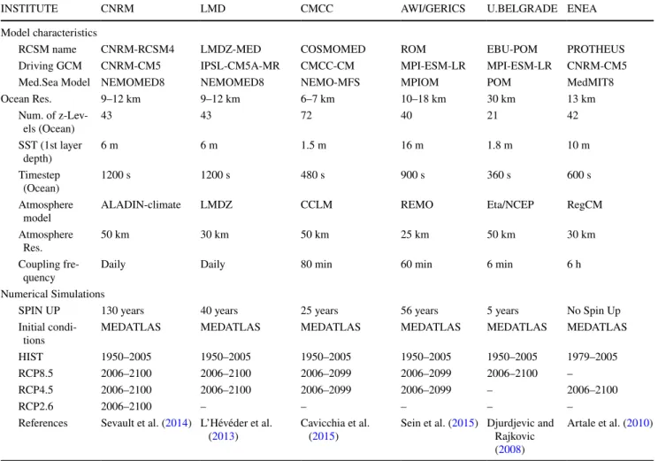
Table 1 Characteristics of the Med-CORDEX coupled regional climate system models (RCSM) and the simulations used in this study

More information on MEDATLAS initial conditions can be found in Rixen et al. (2005)

INSTITUTE CNRM LMD CMCC AWI/GERICS U.BELGRADE ENEA

Model characteristics

RCSM name CNRM-RCSM4 LMDZ-MED COSMOMED ROM EBU-POM PROTHEUS

Driving GCM CNRM-CM5 IPSL-CM5A-MR CMCC-CM MPI-ESM-LR MPI-ESM-LR CNRM-CM5

Med.Sea Model NEMOMED8 NEMOMED8 NEMO-MFS MPIOM POM MedMIT8

Ocean Res. 9–12 km 9–12 km 6–7 km 10–18 km 30 km 13 km

Num. of z-Lev-

els (Ocean) 43 43 72 40 21 42

SST (1st layer

depth) 6 m 6 m 1.5 m 16 m 1.8 m 10 m

Timestep

(Ocean) 1200 s 1200 s 480 s 900 s 360 s 600 s

Atmosphere

model ALADIN-climate LMDZ CCLM REMO Eta/NCEP RegCM

Atmosphere

Res. 50 km 30 km 50 km 25 km 50 km 30 km

Coupling fre-

quency Daily Daily 80 min 60 min 6 min 6 h

Numerical Simulations

SPIN UP 130 years 40 years 25 years 56 years 5 years No Spin Up

Initial condi-

tions MEDATLAS MEDATLAS MEDATLAS MEDATLAS MEDATLAS MEDATLAS

HIST 1950–2005 1950–2005 1950–2005 1950–2005 1950–2005 1979–2005

RCP8.5 2006–2100 2006–2100 2006–2099 2006–2099 2006–2100 –

RCP4.5 2006–2100 2006–2100 2006–2099 2006–2099 – 2006–2100

RCP2.6 2006–2100 – – – – –

References Sevault et al. (2014) L’Hévéder et al.

(2013) Cavicchia et al.

(2015) Sein et al. (2015) Djurdjevic and Rajkovic (2008)

Artale et al. (2010)

(5)

the time being that SST is a reliable sign of possible harmful conditions for deeper layers.

2.2 Reference dataset

In order to evaluate the model’s capability to simulate trends in regional extreme thermal events, we first perform comparisons with satellite data (OBS) provided by the Coperni- cus Marine Service and CNR - ISAC ROME. More specifically, the Mediterranean Sea high-resolution L4 dataset is employed, providing daily, reprocessed SSTs on a 0.04 °grid, an interpolation of remotely sensed SSTs from the Advanced Very High Resolution Radiometer (AVHRR) Pathfinder Ver- sion 5.2 (PFV52) onto a regular grid (Pisano et al. 2016).

They are obtained over a 30-year period of January 1982 to December 2012 and are used as a reference for the models’ performance in the mean and extreme climate in the Mediterranean Sea. With the aim of validating the “present- day” climate, we choose the 30-year period (1976–2005) in the model HIST runs that has the greatest overlap with the observed 30-year period (1982–2012). Prior to perform- ing any calculations and in order to compare the results between the models and observations, we first interpolated every dataset to the NEMOMED8 grid, already in use by 2 RCSMs, by implementing the nearest neighbour method.

2.3 Defining marine heatwaves

As for their atmospheric counterparts, there is no univer- sal definition for MHWs. However, certain metrics can be applied to compare different events in space and time. In this research, the qualitative MHW definition proposed by Hobday et al. (2016) is followed. We use it as a baseline for developing a quantitative method that will identify MHWs, namely in the summer months, based on the climatology and the geographical characteristics of the area. Although we recognise that heatwaves in colder months might also be essential for certain species, we choose to focus on extreme events related to the highest annual SSTs, when organisms may be beyond their optima, as seen by previous mass mortality events in the Mediterranean (e.g. MHW of 1999 and 2003).

According to Hobday et al. (2016) a MHW is a “prolonged, anomalously warm water event at a particular location” and it should be defined relative to a 30-year period.

In our case, a subset of the HIST experiments (1976–2005) and the 1982–2012 period for the observations are chosen, representing the average climate in the latter half of the 20th century. In order to achieve a homogenised yet area-specific temperature diagnostic, for every year of the reference period (HIST) we first compute the 99th quantile of daily SST ( SST_99Q ) for every grid point. Then we average these 30 years of extreme values, constructing a 2D threshold map.

Note that individual threshold maps were created for each dataset separately, accounting for the different model characteristics (e.g SST bias). An “anomalously warm day” at every grid point is then any given day when the local SST_99Q threshold is exceeded. However, in order to be classified as a

“prolonged” event, we set the minimum duration of a MHW to 5 days, following Hobday et al. (2016). Further, we aim to identify long-lasting events, since most of the previous mass mortalities in the basin occurred during thermal anomalies that lasted for more than 5 days (e.g. (Garrabou et al. 2009;

Di Camillo and Cerrano 2015; Cerrano et al. 2000; Cebrian et al. 2011). In addition, the average present-day MHW duration in the basin was found around 10 days (not shown).

Therefore, a 3-day or 7-day minimum definition threshold would not change significantly the MHW characteristics in the future (see Sect. 4.)

The discrete nature of MHWs also necessitates a well- defined starting and ending day, but gaps with temperatures close to threshold values can also be found, as a result of day-to-day SST fluctuations. At this point, our definition dif- fers slightly from that of Hobday et al. (2016). More specifically, gaps of up to 4 consecutive days or less are allowed inside a local MHW (considered as warm days). This is true,however, only when both the preceeding and following 6-day mean SST of a gap day (including the gap day in each mean) are above the local SST_99Q . For the cool day “neigh- bourhood” this would represent a tendency to remain above threshold, even though the SST of that particular cool day might be below limit. This also reflects the fact that minor SST deviations from the threshold cannot impact the overall warm conditions of a MHW. It would most likely not offer either an “essential” relief to organisms, even to the less mobile and perhaps less tolerant species, once a MHW has started. Taking advantage of the default statistical sensitivity of the mean to outliers (in this case cold temperatures), we make the assumption that an event with the potential to interrupt a MHW (e.g wind, current) should cause a consid- erable drop in daily SST. Therefore, a below-threshold drop in either of the 6-day SST averages would not allow any cool day to merge with a MHW, in the same way that a sequence of five cool days or more would interrupt an event entirely.

The 11-day window around the gap day is chosen since the minimum duration of a MHW was set to five days.

The spatial coverage of the MHW is then determined by aggregating grid points that are “activated” in a MHW state every day but are not necessarily contiguous. In common with many atmospheric definitions, a minimum 20%

of the Mediterranean surface in km² was chosen in order to detect large-scale events that may have a broad ecosystem impact but also represent rare occurrence for the average climate conditions of HIST period. We, therefore, opt for prolonged, large-scale and extremely warm ocean temperatures that do not occur on a yearly basis in the 20th century,

(6)

with a view of quantifying their evolution in the 21st century under different GHG emission scenarios. The advantage of a percentile-based SST threshold in our case is that spatial patterns are also identified independently from the different extreme temperature levels that characterise sub-basins in the Mediterranean. We acknowledge that the detection method is developed based on subjective choices, and the sensitivity of the climate change results to these changes was also tested (See Sect. 4).

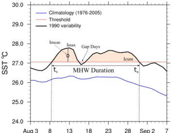
Once a MHW is identified, a subset of MHW metrics defined in Hobday et al. (2016) are used to characterise it. We examine the frequency of MHWs (Annual count of events), and the duration of each event is defined as the time between the first ( t_s ) and last day ( t_e ) for which a minimum of 20% of Mediterranean Sea surface is touched by a MHW. Every event is characterised by a mean and max intensity (mean and spatiotemporal maximum temperature anomaly relative to the threshold over the event duration) and a maximum surface coverage. Finally, its severity is represented by cumulative intensity (spatiotemporal sum of

daily temperature anomalies relative to the threshold over the event duration) (Fig. 1, Table 2)

3 Results

3.1 Model evaluation

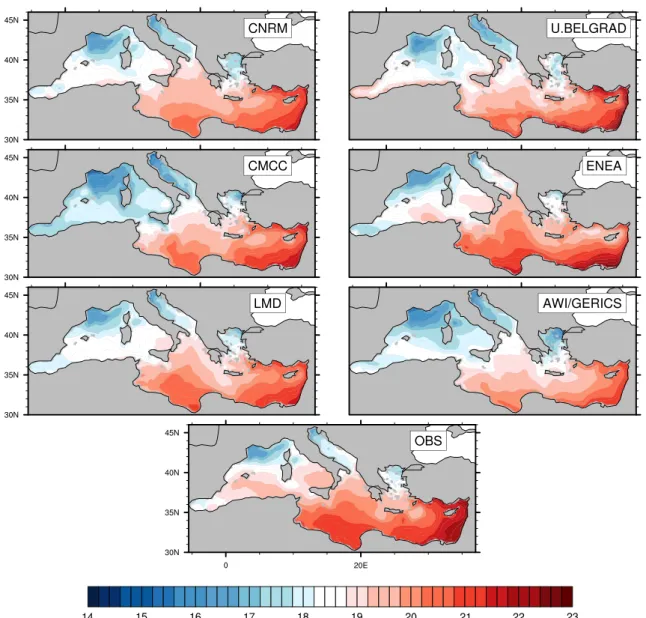
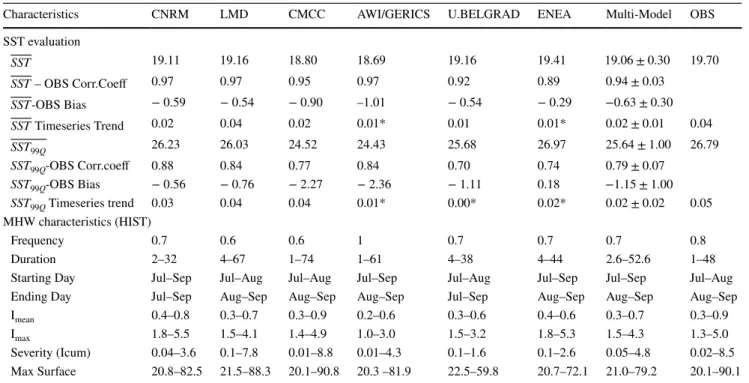
The first goal of this paper is to evaluate each models’ ability to simulate mean ( SST ) and extreme Mediterranean Sea SST ( SST_99Q ) correctly. For this reason, pattern correlations were first performed, using the Pearson product-moment coefficient of linear correlation between two variables. The observed annual mean SST between 1982–2012 (Fig. 2, OBS) shows a NW-SE pattern of cold-warm temperatures ranging from ∼15 °C to 23 °C, respectively. Similarly, all the models demonstrate a warmer Eastern Mediterranean (EM) between 19 and 23 °C while colder deep water formation areas (e.g. Gulf of Lions, Adriatic) are captured well around 15–17 °C. Despite a multi-model mean (MMM) cold bias of about 0.6 °C, spatial correlations between each model mean 1976-2005 SST and observations are high (MMM

∼0.94 ). The lowest bias is found in ENEA and the highest in the CMCC and AWI/GERICS models (see Table 3).

Note that satellite provides skin and night-time SST values, whereas the model SST represents averaged daily temperatures of the first few meters of mixed layer depth. Part of the model bias can be therefore explained by this difference in SST.

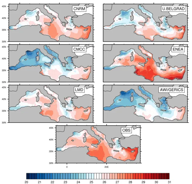
More complex spatial patterns are revealed when exam- ining the 2D threshold maps used as the basis for defining Mediterranean MHWs (Fig. 3). The highest SST_99Q are observed in Central Ionian, Gulf of Gabes, Tyrrhenian Sea and Levantine basin varying from approximately 27–31 °C and the lowest (20–22 °C) in deep water formation areas and the Alboran Sea (Fig. 3 OBS). In general, all the models are able to reproduce these patterns, although this time they share lower spatial correlations with the observations (MMM ∼0.78 ). The ENEA model shows a warm bias whereas CMCC, U.BELGRAD and AWI/GERICS show a cold bias larger than 1 °C. The similar behaviour of the latter three could perhaps be related to the common atmospheric component (ECHAM) of their driving GCM. On the whole, the difference between the MMM mean and the extreme

Fig. 1 Schematic of a MHW based on Hobday et al. (2016). The black line represents daily SST variations of one grid point in a ran- dom year and red line is the local threshold ( SST_99Q ) based on the 30-year average of yearly 99th quantile of daily SST for that point.

The blue line is the daily 30-year climatology for this point. Also shown here also are the starting day ( t_s ) and ending day ( t_e ) above SST_99Q , gap days and the different measures of daily intensity. MHW metrics refer to the total event duration

Table 2 Marine heatwave (MHW) set of properties and their description after Hobday et al. (2016)

Marine Heatwave Metrics Description

Frequency Number of events occurring per year

Duration (t_e – t_s ) +1 (days)

Mean intensity (I_mean) ∫ [ ∫(SST_(x,y,t) – SST_99Q(x,y))dxdy]dt/∫dxdy∫ dt (°C) Max intensity (I_max) max_(x,y,t)(SST_(x,y,t) − SST_99Q(x,y) ) (°C)

Severity (Icum) ∫ [ ∫(SST_(x,y,t) − SST_99Q(x,y))dxdy]dt (°C days km²)

(7)

basinwide SST is found to be ∼6.6 °C, in good agreement with the observations (7.1 °C). The corresponding MMM spread is small for the SST but higher for the SST_99Q ( ∼1

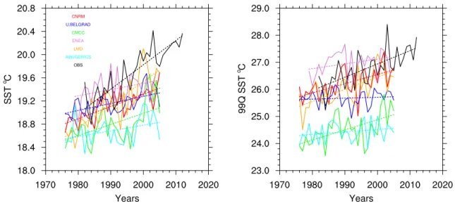
°C).Further, the domain-averaged timeseries of SST illustrate a warming tendency of both the SST and annual SST_99Q (Fig. 4; Table 3). Even though MMM SST and SST_99Q obtain similar trends ( ∼0.02 °C/year) they seem to underestimate the corresponding observed trends (0.04/0.05 °C/year).

Particularly for AWI/GERICS and U.BELGRAD, this is a response likely explained by their common driving GCM (MPI-ESM-LR). On the other hand, the amplitude of interannual variability is found similar to the observations for most of the models. On the whole, the observed and most of the model trends are statistically significant at a level of

95% except for certain cases indicated in Table 3. Interest- ingly, none of the simulations peaked as high as the observations during the exceptional MHW year of 2003 (20.4 °C for SST and 28.4 °C for SST_99Q ). This record basinwide SST_99Q value is on average 8.7 °C higher than the average SST °C of 1982–2012 and 2.8 °C greater than the basin-mean SST_99Q of that period.

In terms of MHW properties during 1982–2012 (Table 3), observed MHW frequency is found at 0.8 events per year that last a maximum of 1.5 months and range between July and September. The mean intensity of MHWs varies from 0.3 to 0.9 °C, covering a maximum of 20–90% of the Medi- terranean Sea surface, with a maximum intensity of 5.0 °C (2002) and a maximum severity of 8.5×10⁷ ° C days km² . The highest values over this period (except from I_max) refer

Fig. 2 Yearly SST (°C) for the HIST run of every model (1976–2005) and satellite data during 1982–2012. Note that the HIST run for ENEA is from 1979–2005

(8)

to the characteristics of the well-known MHW 2003. More specifically, they correspond to a Mediterranean-scale event lasting 48 days (20 July–5 September) by our definition, in line with Grazzini and Viterbo (2003) and Sparnocchia et al.

(2006). It seems that mainly the phase of the MHW that was both large-scale and intense was captured here.

On average, the simulated events during HIST are well within the equivalent observed range of every variable. They manifest though a slightly lower annual frequency, a potential for slightly higher maximum durations and starting dates up to early September. They also appear to underestimate the upper level of the I_mean, I_max and severity range. In particular, event durations of two months or more are exhibited by LMD, CMCC and AWI/GERICS models, while the ENEA model shows the highest I_max of 5.3 °C. Maximum severity,

on the other hand, appears closer to the observed values only in the LMD and CMCC models. These configurations also show a MHW maximum spatial coverage above 80%, along with CNRM and AWI/GERICS. In general, the Med-COR- DEX ensemble appears to perform well given that this is the first time, to our knowledge, that Mediterranean RCSMs have been evaluated for MHWs properties.

To better understand the ensemble variability of the MHW characteristics in the HIST period, we also com- bine Intensity-Duration-Frequency (IDF) information for every dataset separately (see Fig. 5). The total number of events of this period are organised in bins of I_mean (every 0.02 °C) and duration (5-day bins progressively increased to 10-day and 20-day bins). Although some models simulate longer events relative to the observed MHW 2003,

Fig. 3 Individual MHW threshold maps of mean SST_99Q (°C) computed from the HIST run of every model (1976–2005) and satellite data during 1982–2012. Note that the HIST run for ENEA is from 1979–2005

(9)

only CMCC exhibited equivalent MHWs in terms of duration and intensity. At the same time, 1–3 events are detected for most classes of I_mean and duration, in both the observations and the models. There are only a few cases where 3–7 events appear with I_mean below 0.6 °C but follow no specific duration pattern.

3.2 Future Mediterranean SST evolution

In this section we analyze projections of SST and SST_99Q in the 21st century by comparing their evolution against the reference period and under different GHG emission scenarios.

Fig. 4 Timeseries of area-averaged, yearly SST °C (left) and SST_99Q °C (right), during HIST for every model and satellite data, represented by a solid line. Trends are indicated in dashed lines. The different simulations are represented by different colors

Fig. 5 IDF plot; Intensity (I_mean in °C), Duration (Days), Frequency (Number of MHW during 1976–2005). I_mean is organised in bins of 0.02 °C while duration is in bins of 5, 10 and 20 days. Red box indicates observed characteristics corresponding to the exceptional MHW of 2003

(10)

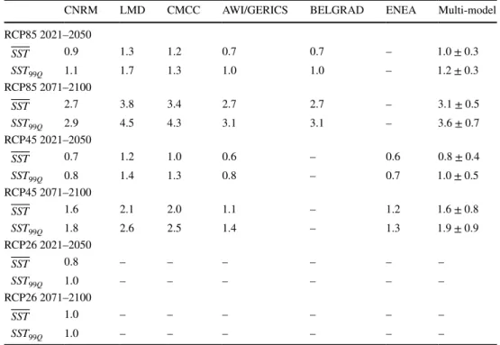
During 2021–2050 an increase is found for the domain- averaged ensemble mean SST and SST_99Q with respect to HIST, around 0.8–1 °C and 1–1.2 °C respectively. While

the mid-21st century anomalies appear almost independent from the greenhouse gas forcing, a more diverse and substantial warming occurs towards 2071–2100 (see Fig. 6).

Table 3 Evaluation of SST and MHW properties during HIST run

Mean annual and threshold SST are indicated with SST (°C) and SST_99Q (°C) respectively. The Mann-Kendal non-parametric test is used to detect the presence of linear or non-linear monotonic trends (°C/year) in domain-averaged SST timeseries. Trends with statistical significance lower than 95% level are indicated with star. Spatial correlations (Corr.Coeff) and bias with respect to observations are given for each dataset.

Also shown here, are the range (min and max) of frequency, duration (days), starting day (calendar month), ending day (calendar month), I_mean (°C) I_max (°C), Severity*10⁷ (°C days km² ) and maximum surface coverage(%) of MHWs. The multi-model column indicates the ensemble average values and standard deviation for each variable

Characteristics CNRM LMD CMCC AWI/GERICS U.BELGRAD ENEA Multi-Model OBS

SST evaluation

SST 19.11 19.16 18.80 18.69 19.16 19.41 19.06±0.30 19.70

SST – OBS Corr.Coeff 0.97 0.97 0.95 0.97 0.92 0.89 0.94±0.03

SST-OBS Bias − 0.59 − 0.54 − 0.90 –1.01 − 0.54 − 0.29 −0.63±0.30

SST Timeseries Trend 0.02 0.04 0.02 0.01* 0.01 0.01* 0.02±0.01 0.04

SST_99Q 26.23 26.03 24.52 24.43 25.68 26.97 25.64±1.00 26.79

SST_99Q-OBS Corr.coeff 0.88 0.84 0.77 0.84 0.70 0.74 0.79±0.07

SST_99Q-OBS Bias − 0.56 − 0.76 − 2.27 − 2.36 − 1.11 0.18 −1.15±1.00

SST_99Q Timeseries trend 0.03 0.04 0.04 0.01* 0.00* 0.02* 0.02±0.02 0.05

MHW characteristics (HIST)

Frequency 0.7 0.6 0.6 1 0.7 0.7 0.7 0.8

Duration 2–32 4–67 1–74 1–61 4–38 4–44 2.6–52.6 1–48

Starting Day Jul–Sep Jul–Aug Jul–Aug Jul–Sep Jul–Aug Jul–Sep Jul–Sep Jul–Aug

Ending Day Jul–Sep Aug–Sep Aug–Sep Aug–Sep Jul–Sep Aug–Sep Aug–Sep Aug–Sep

I_mean 0.4–0.8 0.3–0.7 0.3–0.9 0.2–0.6 0.3–0.6 0.4–0.6 0.3–0.7 0.3–0.9

I_max 1.8–5.5 1.5–4.1 1.4–4.9 1.0–3.0 1.5–3.2 1.8–5.3 1.5–4.3 1.3–5.0

Severity (Icum) 0.04–3.6 0.1–7.8 0.01–8.8 0.01–4.3 0.1–1.6 0.1–2.6 0.05–4.8 0.02–8.5

Max Surface 20.8–82.5 21.5–88.3 20.1–90.8 20.3 –81.9 22.5–59.8 20.7–72.1 21.0–79.2 20.1–90.1

Fig. 6 Area-average, yearly SST °C (left) and extreme SST_99Q °C

(right) anomalies with respect to HIST. Bold colors represent the multi-model average and lighter colors are the individual simulations.

RCP2.6 scenario has only one simulation (CNRM), HIST run is illustrated in grey and observations in dashed black

(11)

In particular, the multi-model mean SST and SST_99Q anomalies under RCP8.5 are 3.1 °C and 3.6 °C respectively, exhibiting nearly a doubling of their corresponding RCP4.5 rise. Similarly, the equivalent increase of CNRM SST and SST_99Q under RCP8.5 is about 3 times as high as that under RCP2.6 for the same period. Individually, however, the highest mean and extreme SST anomalies are demonstrated by the LMD and CMCC models under every scenario and for every period (see Table 4). For both SST indices, the effects of the different emission scenarios become more evident by 2060, with the highest/

intermediate warming occurring for every model under RCP8.5/RCP4.5 and the lowest under the (mono-model) RCP2.6 simulation. In the latter, little or no difference is found between the SST and SST_99Q rise throughout the century. In contrast, under RCP4.5 and RCP8.5, the multi- model SST_99Q increase appears greater than the SST rise by 20–25% during 2021–2050 and by 16–18% for 2071–2100 (see Table 4 and discussion section). This implies a higher contribution from SST to the warming towards the end of the century.

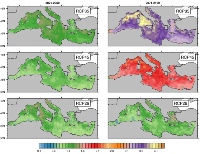
The spatial distribution of the corresponding anomalies, however, appears inhomogeneous. For 2071–2100, some regions in the Levantine basin, Balearic islands, Tyrrenian Sea, Ionian Sea and North Adriatic Sea exhibit the highest MMM SST anomalies in every scenario (Fig. 7). In contrast, the lowest anomalies of that time are located in the Alboran Sea, where cold waters are advected from the

Atlantic, and depending on the scenario they may range from ∼0.6 °C (RCP2.6) to ∼2.4 °C (RCP8.5).

Meanwhile, the most pronounced extreme warm anomalies ( SST_99Q ) for 2071–2100 under RCP4.5 and RCP8.5 are projected for the NW mediterranean, Tyrrenian Sea, Ionian Sea and some parts of North Levantine basin (Fig. 8). Under RCP2.6 though, the greatest SST_99Q anomalies (> 1.2 °C) are more confined towards the Aegean Sea, Adriatic, Tyr- rhenian Sea and the area around Balearic islands. In addition to the highest SST_99Q rise, the Adriatic Sea, Ionian Sea, Tyr- rhenian Sea, some parts around the Balearic islands and the North Levantine basin display also the greatest SST rise, for every scenario during the 2nd half of the 21st century. Dur- ing 2021–2050, however, they exhibit the highest mean and extreme warming under RCP26 and RCP4.5 but not under RCP8.5. The Alboran Sea and the SE Levantine basin, on the other hand, demonstrate the lowest SST_99Q anomalies in every period and every scenario

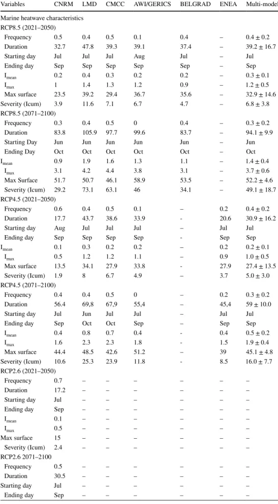
3.3 Future evolution of Mediterranean MHWs The MHW climate change response is examined here using anomalies. These anomalies are computed for the average MHW characteristics in the future relative to the average MHW characteristics in HIST run, for each sub-period, model and scenario (Table 5).

The multi-model mean reveals an increase in frequency of 0.3–0.4 events/year for every period of RCP4.5/RCP8.5 with the mono-model RCP2.6 simulation showing a

Table 4 Future Mediterranean- averaged, yearly mean ( SST ) and extreme ( SST_99Q ) anomalies (with respect to HIST) for the near and far future under different emission scenarios

The multi-model column indicates the ensemble average values and standard deviation. Values are in °C

CNRM LMD CMCC AWI/GERICS BELGRAD ENEA Multi-model

RCP85 2021–2050

SST 0.9 1.3 1.2 0.7 0.7 – 1.0±0.3

SST_99Q 1.1 1.7 1.3 1.0 1.0 – 1.2±0.3

RCP85 2071–2100

SST 2.7 3.8 3.4 2.7 2.7 – 3.1±0.5

SST_99Q 2.9 4.5 4.3 3.1 3.1 – 3.6±0.7

RCP45 2021–2050

SST 0.7 1.2 1.0 0.6 – 0.6 0.8±0.4

SST_99Q 0.8 1.4 1.3 0.8 – 0.7 1.0±0.5

RCP45 2071–2100

SST 1.6 2.1 2.0 1.1 – 1.2 1.6±0.8

SST_99Q 1.8 2.6 2.5 1.4 – 1.3 1.9±0.9

RCP26 2021–2050

SST 0.8 – – – – – –

SST_99Q 1.0 – – – – – –

RCP26 2071–2100

SST 1.0 – – – – – –

SST_99Q 1.0 – – – – – –

(12)

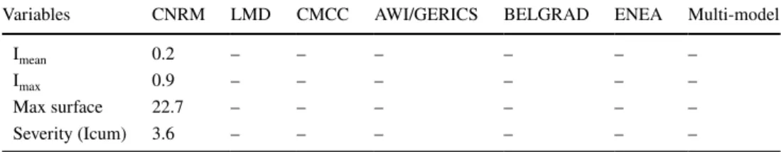
Table 5 Future response (anomalies with respect to HIST) of MHW mean properties for the 6 RCSMs under RCP8.5, RCP4.5 and RCP2.6, for the near (2021- 2050) and far future (2071–

2100).

Variables CNRM LMD CMCC AWI/GERICS BELGRAD ENEA Multi-model

Marine heatwave characteristics RCP8.5 (2021–2050)

Frequency 0.5 0.4 0.5 0.1 0.4 – 0.4±0.2

Duration 32.7 47.8 39.3 39.1 37.4 – 39.2±16.7

Starting day Jul Jul Jul Aug Jul – Jul

Ending day Sep Sep Sep Sep Sep – Sep

I_mean 0.2 0.4 0.3 0.2 0.2 – 0.3±0.1

I_max 1 1.4 1.3 1.2 0.9 – 1.2±0.5

Max surface 23.5 39.2 29.4 36.7 35.6 – 32.9±14.6

Severity (Icum) 3.9 11.6 7.1 6.7 4.7 – 6.8±3.8

RCP8.5 (2071–2100)

Frequency 0.3 0.4 0.5 0 0.4 – 0.3±0.2

Duration 83.8 105.9 97.7 99.6 83.7 – 94.1±9.9

Starting Day Jun Jun Jun Jun Jun – Jun

Ending Day Oct Oct Oct Oct Oct – Oct

I_mean 0.9 1.9 1.6 1.3 1.1 – 1.4±0.4

I_max 3.1 4.2 4.4 3.8 3.1 – 3.7±0.6

Max Surface 51.7 50.7 46.1 58.9 53.5 – 52.2±4.6

Severity (Icum) 29.2 73.1 63.1 46 34.1 – 49.1±18.7

RCP4.5 (2021–2050)

Frequency 0.6 0.4 0.5 0.1 – 0.2 0.4±0.2

Duration 17.7 43.7 38.6 33.9 - 20.6 30.9±16.2

Starting day Aug Jul Jul Jul – Jul Jul

Ending day Sep Sep Sep Sep - Sep Sep

I_mean 0.1 0.3 0.2 0.2 – 0.2 0.2±0.1

I_max 0.5 1.2 1.2 1.1 – 0.9 1.0±0.5

Max surface 13.5 34.1 27.9 33.8 - 27.9 27.4±13.5

Severity (Icum) 1.9 8 6.7 4.9 – 3.7 5.0±3.0

RCP4.5 (2071–2100)

Frequency 0.4 0.4 0.5 0 – 0.2 0.3±0.2

Duration 56.4 69,8 67,9 55,4 – 45,4 59±10.0

Starting day Jul Jun Jul Jul – Jul Jul

Ending day Sep Oct Oct Sep – Sep Sep

I_mean 0.4 0.8 0.7 0.4 - 0.4 0.5±0.2

I_max 1.6 2.3 2.3 1.8 - 1.5 1.9±0.4

Max surface 44.4 48.5 42.6 51.2 – 39 45.1±4.8

Severity (Icum) 10.6 25.3 23.9 11.8 - 8.5 16.0±7.7

RCP2.6 (2021–2050)

Frequency 0.7 – – – – – –

Duration 17.2 – – – – – –

Starting day Jul – – – – – –

Ending day Sep – – – – – –

I_mean 0.1 – – – – – –

I_max 0.5 – – – – – –

Max surface 15 – – – – – –

Severity (Icum) 2.4 – – – – – –

RCP2.6 2071–2100

Frequency 0.5 – – – – – –

Duration 30.5 – – – – – –

Starting day Jul – – – – – –

Ending day Sep – – – – – –

(13)

slightly greater increase of 0.5–0.7 events/year. In fact, individual simulations of Fig. 9 suggest a shift from a period where years without MHWs were common (1976–2030) to a period with at least one long-lasting MHW every year. More specifically, towards 2071–2100, events can start as early as June and finish as late as Octo- ber under RCP8.5, whereas for RCP4.5 and RCP2.6, the MHW temporal extent appears between July–September (Fig. 10). It is clear that the higher the radiative forcing, the broader the window of occurrence. For example,

MHWs during 2071–2100 may last on average 3 months longer in RCP8.5 than HIST MHWs ( ∼21.8 days, not shown) but almost 2 months longer in RCP4.5 (see Table 5). This is a MMM increase in the duration, almost double the corresponding increase during 2021–2050 under RCP4.5 ( ∼30.9 days) and more than double that under RCP8.5 ( ∼39.2 days). Even under the optimistic RCP2.6 scenario, MHWs by 2050 may be 17.2 days longer than today and may become 1 month longer at maximum by 2100.

Shown here are the average annual event count (frequency), average MHW duration (days), starting day (calendar month), ending day (calendar month), I_mean (°C), I_max (°C), severity ( ∗10⁷ ° C days km² ) and maximum surface coverage (%). The multi-model column indicates the ensemble mean values for each variable and their standard deviation. Only the CNRM simulation is available for the RCP2.6 scenario, 5 simulations for RCP8.5 and 5 simulations for RCP4.5

Table 5 (continued) Variables CNRM LMD CMCC AWI/GERICS BELGRAD ENEA Multi-model

I_mean 0.2 – – – – – –

I_max 0.9 – – – – – –

Max surface 22.7 – – – – – –

Severity (Icum) 3.6 – – – – – –

Fig. 7 Multi-model average anomaly of yearly SST (°C) with respect to the corresponding ensemble mean HIST of each scenario, for the near and far future. The RCP2.6 scenario has only one simulation (CNRM)

(14)

Long-term projections show analogous changes in the I_mean of future MHWs. They are examined through IDF plots that display the total number of MHWs identified by the ensemble during HIST (1976–2005) run, near and far future (Fig. 11). To avoid imbalances in the present-future comparisons arising from the different sets of models for

Fig. 8 Multi-model average anomaly of extreme SST_99Q (°C) with respect to corresponding ensemble mean HIST (1976-2005) of each scenario, for the near and far future. The RCP2.6 scenario has only one simulation (CNRM)

Fig. 9 Annual number of MHWs (Annual Frequency) for RCP8.5 (red) RCP4.5 (blue) RCP2.6 (green) HIST (grey) and observations (dashed black). Bold colors indicate the multi-model mean and shaded zones represent individual MHW events identified by the models. Years without MHWs are also included, with shaded areas reaching 0. RCP2.6 has only 1 simulation (CNRM)

Fig. 10 Annual earliest starting (solid lines) and latest ending (dashed lines) day of MHW events for RCP8.5 (red) RCP4.5 (blue) RCP2.6 (green) HIST (grey) and observations (black). Bold colors indicate multi-model average values while lighter dots represent individual event dates

(15)

RCP4.5 and RCP8.5 (see Table 5), all the simulated future events are pooled for every period and juxtaposed against the corresponding sets of HIST events. Therefore, we show 3 HIST IDF plots, one for each scenario. As previously demonstrated the stronger the emission scenario, the longer the duration and the higher the I_mean of the events. The MMM I_mean response appears small during 2021–2050 (+ 0.1°C to + 0.3 °C depending on the scenario) but increases towards

the end of the period with higher radiative forcing. For instance, MHWs show durations of up to 170 days (Fig. 11) in the far future of RCP8.5 and I_mean of 1.8 °C on average (not shown). For the CNRM model though and under RCP2.6, the corresponding response towards 2071–2100 has doubled compared to the mid-21st century, while it becomes 4.5 times higher under RCP8.5 (see Table 5). Longer-lasting MHWs at the end of the period for RCP4.5 and RCP8.5

Fig. 11 IDF (I_mean, Duration, Frequency) plots display the total MHW number of every dataset, for every scenario, over 2021-2050 and 2071-2100. RCP8.5 and RCP4.5 include events from 5 simulations, while RCP2.6 from only 1 (CNRM) simulation. HIST run contains

MHWs from the corresponding set of models each time. The number of MHWs is calculated over each 30 year period. For contrast purposes, the red box depicts the observed characteristics of MHW 2003 in the Mediterranean

(16)

explain the lower frequency of occurrences compared to RCP2.6. A similar behaviour to I_mean displays the MMM average response of I_max, with the highest anomalies indicated towards 2071–2100 (up to 3.7 °C), whereas during the mid-21st century they range between 0.5 °C (RCP2.6) and 1.2 °C(RCP8.5).

It should be also noted that for RCP4.5 and RCP8.5, events with characteristics similar to the observed exceptional MHW 2003 (Fig. 11, red box) seem to become the new standard over 2021–2050 and even constitute weak occurrences for the distant future of RCP8.5. In the more optimistic RCP2.6, MHWs appear more frequent during 2021–2050 but their number is slightly decreased towards 2071–2100. Their characteristics, however, sustain a lower increase throughout the period compared to RCP4.5 and RCP8.5. For example, the response in duration and I_mean is found close to that projected for CNRM during 2021–2050 and under RCP4.5 and RCP8.5 (see Table 5). Therefore, the possibility for an event like the MHW 2003 to occur regu- larly still features in a scenario close to the Paris Agreement (RCP2.6) .

Yet, the range of the uncertainty in future projections evolves not only in time but also throughout the different models. The severity (Icum) distribution of future MHWs was determined in that sense using Whisker diagrams.

In these box plots, a specific Icum index is appointed at each simulated event of every dataset for each period and scenario (see Fig. 12, left). By definition, Icum translates the total spatiotemporal MHW impact into numbers. It features an exponential increase from HIST towards the

end of the century from ∼1×10⁷C days km² to about

∼50×10⁷C days km² for RCP8.5 (2071–2100-not shown). Moreover, the higher the emission forcing, the higher the rate the ensemble mean Icum response esca- lates from its mid- to end-of-century values; for example, Icum varies from 5 to 33×10⁷C days km² in RCP4.5 and from 6.8 to 49.1×10⁷C days km² in RCP8.5 (see Table 5).

This becomes more evident when comparing the equivalent CNRM severity response under RCP2.6 (2.4–3.6 × 10⁷C days km² ) with the significantly higher response under RCP4.5 and RCP8.5. Although all configurations indicate an abrupt escalation through time, there appears to be a family of models (CMCC and LMD) that share a stronger climate change response. Those models exhibit higher changes in Icum, along with higher I_mean, I_max, and duration values than the remaining models (see also Table 5 and Sect. 4).

The identified families of MHWs are also associated with a maximum spatial coverage illustrated through box plots in Fig. 12. It is estimated that events may affect a maximum of 40% of the Mediterranean Sea, on average, during HIST but may impact almost 100% of the basin by 2071–2100 under RCP8.5. Notwithstanding the large variability found for the mid-21st century, by 2100 the simulated maximum MHW extent seems to be an unani- mous projection from every model and under RCP8.5.

Conversely, MHWs under RCP2.6 increase their maximum coverage throughout the period, but towards 2071–2100 events may impact, on average, a maximum of 70% of the Mediterranean Sea.

Fig. 12 Whisker diagram of (left) Severity (Icum) and (right) maximum surface coverage of every observed and simulated MHW during HIST, 2021-2050 and 2071-2100. Box plots illustrate minimum, 25th

percentile, median, 75th percentile and maximum values of each variable for a given model, scenario and period