Ensemble Data Assimilation
Algorithms – Applications – Software
Lars Nerger
Alfred Wegener Institute Helmholtz Center for Polar and Marine Research Bremerhaven, Germany
Acknowledgements:
W. Hiller, J. Schröter, S. Losa, A. Androsov, H. Pradhan, M. Goodliff, Q. Tang, Q. Yang, L. Mu
SPP1788 Colloquium 2019, Bad Aibling, 3.-6.6.2019
Lars Nerger – Ensemble Data Assimilation
• Generally correct, but has errors
• all fields, fluxes on model grid
• Generally correct, but has errors
• incomplete information:
data gaps, some fields
ocean data: mainly surface (satellite) Combine both sources of information
quantitatively by computer algorithm
➜ Data Assimilation
Motivation
Information: Model Information: Observations
Model surface temperature Satellite surface temperature
Lars Nerger – Ensemble Data Assimilation
Data Assimilation
Methodology to combine model with real data
§ Optimal estimation of system state:
• initial conditions (for weather/ocean forecasts, …)
• state trajectory (temperature, concentrations, …)
• parameters (ice strength, plankton growth, …)
• fluxes (heat, primary production, …)
• boundary conditions and forcing (wind stress, …)
§ More advanced: Improvement of model formulation
• Detect systematic errors (bias)
• Revise parameterizations based on parameter estimates
€
Lars Nerger – Ensemble Data Assimilation
Interdisciplinarity of Data Assimilation
€
Data
Assimilation
Algorithms Applications
Software
Mathematics:
Optimization Estimation Inverse problems
Numerics
Earth Sciences, Physics,
Biology,
Cognitive science, ...
Computer Science:
High-performance computing Big data
Machine learning
Lars Nerger – Ensemble Data Assimilation
Outline
Ensemble Data Assimilation
Algorithms / Methodology
• Efficient methods for high-dimensional nonlinear systems Applications
• Examples of what one can expect to achieve Software
• Make ensemble data assimilation easily usable
• Parallel Data Assimilation Framework (PDAF)
Lars Nerger – Ensemble Data Assimilation
Methodology
Lars Nerger – Ensemble Data Assimilation
Data Assimilation – a general view
Consider some physical system (ocean, atmosphere, land, …)
time
observation truth
model
state Variational assimilation
Sequential assimilation Two main approaches:
Goal: Obtain optimal estimate of system
constrained by model dynamics and observations
Estimate not necessarily between model and obs.
due to model dynamics
Assimilation
estimate
Lars Nerger – Ensemble Data Assimilation
Needed for Data assimilation
1. Model
• with some skill
2. Observations
• with finite errors
• related to model fields
3. Data assimilation method
€
Lars Nerger – Ensemble Data Assimilation
Models
Simulate dynamics, e.g. the ocean
§ Numerical formulation of relevant terms
§ Discretization with finite resolution in time and space
§ “forced” by external sources (atmosphere, river inflows)
§ Uncertainties
• initial model fields
• external forcing
• in predictions due to model formulation
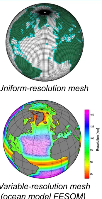
Uniform-resolution mesh
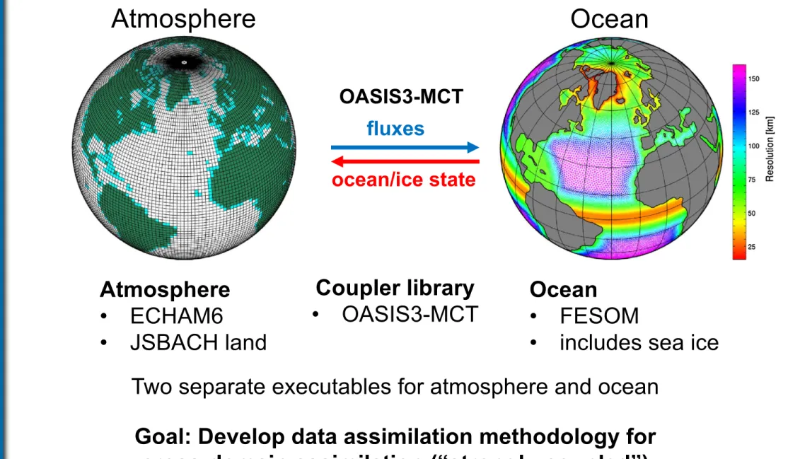
759ECHAM6–FESOM: model formulation and mean climate
1 3
2013) and uses total wavenumbers up to 63, which corre- sponds to about 1.85×1.85 degrees horizontal resolution;
the atmosphere comprises 47 levels and has its top at 0.01 hPa (approx. 80 km). ECHAM6 includes the land surface model JSBACH (Stevens et al. 2013) and a hydrological discharge model (Hagemann and Dümenil 1997).
Since with higher resolution “the simulated climate improves but changes are incremental” (Stevens et al.
2013), the T63L47 configuration appears to be a reason- able compromise between simulation quality and compu- tational efficiency. All standard settings are retained with the exception of the T63 land-sea mask, which is adjusted to allow for a better fit between the grids of the ocean and atmosphere components. The FESOM land-sea distribu- tion is regarded as ’truth’ and the (fractional) land-sea mask of ECHAM6 is adjusted accordingly. This adjustment is accomplished by a conservative remapping of the FESOM land-sea distribution to the T63 grid of ECHAM6 using an adapted routine that has primarily been used to map the land-sea mask of the MPIOM to ECHAM5 (H. Haak, per- sonal communication).
2.2 The Finite Element Sea Ice-Ocean Model (FESOM) The sea ice-ocean component in the coupled system is represented by FESOM, which allows one to simulate ocean and sea-ice dynamics on unstructured meshes with variable resolution. This makes it possible to refine areas of particular interest in a global setting and, for example, resolve narrow straits where needed. Additionally, FESOM allows for a smooth representation of coastlines and bottom topography. The basic principles of FESOM are described by Danilov et al. (2004), Wang et al. (2008), Timmermann et al. (2009) and Wang et al. (2013). FESOM has been validated in numerous studies with prescribed atmospheric forcing (see e.g., Sidorenko et al. 2011; Wang et al. 2012;
Danabasoglu et al. 2014). Although its numerics are fun- damentally different from that of regular-grid models,
previous model intercomparisons (see e.g., Sidorenko et al.
2011; Danabasoglu et al. 2014) show that FESOM is a competitive tool for studying the ocean general circulation.
The latest FESOM version, which is also used in this paper, is comprehensively described in Wang et al. (2013). In the following, we give a short model description here and men- tion those settings which are different in the coupled setup.
The surface computational grid used by FESOM is shown in Fig. 1. We use a spherical coordinate system with the poles over Greenland and the Antarctic continent to avoid convergence of meridians in the computational domain. The mesh has a nominal resolution of 150 km in the open ocean and is gradually refined to about 25 km in the northern North Atlantic and the tropics. We use iso- tropic grid refinement in the tropics since biases in tropi- cal regions are known to have a detrimental effect on the climate of the extratropics through atmospheric teleconnec- tions (see e.g., Rodwell and Jung 2008; Jung et al. 2010a), especially over the Northern Hemisphere. Grid refinement (meridional only) in the tropical belt is employed also in the regular-grid ocean components of other existing climate models (see e.g., Delworth et al. 2006; Gent et al. 2011).
The 3-dimensional mesh is formed by vertically extending the surface grid using 47 unevenly spaced z-levels and the ocean bottom is represented with shaved cells.
Although the latest version of FESOM (Wang et al.
2013) employs the K-Profile Parameterization (KPP) for vertical mixing (Large et al. 1994), we used the PP scheme by Pacanowski and Philander (1981) in this work. The rea- son is that by the time the coupled simulations were started, the performance of the KPP scheme in FESOM was not completely tested for long integrations in a global setting.
The mixing scheme may be changed to KPP in forthcom- ing simulations. The background vertical diffusion is set to 2×10⁻³m2s−1 for momentum and 10−5m2s−1 for potential temperature and salinity. The maximum value of vertical diffusivity and viscosity is limited to 0.01 m2s−1. We use the GM parameterization for the stirring due to
Fig. 1 Grids correspond- ing to (left) ECHAM6 at T63 (≈180 km) horizontal resolu- tion and (right) FESOM. The grid resolution for FESOM is indicated through color coding (in km). Dark green areas of the T63 grid correspond to areas where the land fraction exceeds 50 %; areas with a land fraction between 0 and 50 % are shown in light green
759 ECHAM6–FESOM: model formulation and mean climate
1 3
2013) and uses total wavenumbers up to 63, which corre- sponds to about 1.85×1.85 degrees horizontal resolution;
the atmosphere comprises 47 levels and has its top at 0.01 hPa (approx. 80 km). ECHAM6 includes the land surface model JSBACH (Stevens et al. 2013) and a hydrological discharge model (Hagemann and Dümenil 1997).
Since with higher resolution “the simulated climate improves but changes are incremental” (Stevens et al.
2013), the T63L47 configuration appears to be a reason- able compromise between simulation quality and compu- tational efficiency. All standard settings are retained with the exception of the T63 land-sea mask, which is adjusted to allow for a better fit between the grids of the ocean and atmosphere components. The FESOM land-sea distribu- tion is regarded as ’truth’ and the (fractional) land-sea mask of ECHAM6 is adjusted accordingly. This adjustment is accomplished by a conservative remapping of the FESOM land-sea distribution to the T63 grid of ECHAM6 using an adapted routine that has primarily been used to map the land-sea mask of the MPIOM to ECHAM5 (H. Haak, per- sonal communication).
2.2 The Finite Element Sea Ice-Ocean Model (FESOM) The sea ice-ocean component in the coupled system is represented by FESOM, which allows one to simulate ocean and sea-ice dynamics on unstructured meshes with variable resolution. This makes it possible to refine areas of particular interest in a global setting and, for example, resolve narrow straits where needed. Additionally, FESOM allows for a smooth representation of coastlines and bottom topography. The basic principles of FESOM are described by Danilov et al. (2004), Wang et al. (2008), Timmermann et al. (2009) and Wang et al. (2013). FESOM has been validated in numerous studies with prescribed atmospheric forcing (see e.g., Sidorenko et al. 2011; Wang et al. 2012;
Danabasoglu et al. 2014). Although its numerics are fun- damentally different from that of regular-grid models,
previous model intercomparisons (see e.g., Sidorenko et al.
2011; Danabasoglu et al. 2014) show that FESOM is a competitive tool for studying the ocean general circulation.
The latest FESOM version, which is also used in this paper, is comprehensively described in Wang et al. (2013). In the following, we give a short model description here and men- tion those settings which are different in the coupled setup.
The surface computational grid used by FESOM is shown in Fig. 1. We use a spherical coordinate system with the poles over Greenland and the Antarctic continent to avoid convergence of meridians in the computational domain. The mesh has a nominal resolution of 150 km in the open ocean and is gradually refined to about 25 km in the northern North Atlantic and the tropics. We use iso- tropic grid refinement in the tropics since biases in tropi- cal regions are known to have a detrimental effect on the climate of the extratropics through atmospheric teleconnec- tions (see e.g., Rodwell and Jung 2008; Jung et al. 2010a), especially over the Northern Hemisphere. Grid refinement (meridional only) in the tropical belt is employed also in the regular-grid ocean components of other existing climate models (see e.g., Delworth et al. 2006; Gent et al. 2011).
The 3-dimensional mesh is formed by vertically extending the surface grid using 47 unevenly spaced z-levels and the ocean bottom is represented with shaved cells.
Although the latest version of FESOM (Wang et al.
2013) employs the K-Profile Parameterization (KPP) for vertical mixing (Large et al. 1994), we used the PP scheme by Pacanowski and Philander (1981) in this work. The rea- son is that by the time the coupled simulations were started, the performance of the KPP scheme in FESOM was not completely tested for long integrations in a global setting.
The mixing scheme may be changed to KPP in forthcom- ing simulations. The background vertical diffusion is set to 2×10⁻³m2s−1 for momentum and 10−5m2s−1 for potential temperature and salinity. The maximum value of vertical diffusivity and viscosity is limited to 0.01 m2s−1. We use the GM parameterization for the stirring due to
Fig. 1 Grids correspond- ing to (left) ECHAM6 at T63 (≈180 km) horizontal resolu- tion and (right) FESOM. The grid resolution for FESOM is indicated through color coding (in km). Dark green areas of the T63 grid correspond to areas where the land fraction exceeds 50 %; areas with a land fraction between 0 and 50 % are shown in light green