A Survey on Economic-driven Evaluations of Information Technology

(1)

A Survey on Economic-driven Evaluations of Information Technology

Bela Mutschler, Novica Zarvi´c

^∗

, Manfred Reichert University of Twente, Information Systems Group {b.b.mutschler,n.zarvic,m.u.reichert}@utwente.nl

Abstract

The economic-driven evaluation of information technol- ogy (IT) has become an important instrument in the man- agement of IT projects. Numerous approaches have been developed to quantify the costs of an IT investment and its assumed profit, to evaluate its impact on business process performance, and to analyze the role of IT regarding the achievement of enterprise objectives. This paper discusses approaches for evaluating IT from an economic-driven per- spective. Our comparison is based on a framework distin- guishing between classification criteria and evaluation cri- teria. The former allow for the categorization of evaluation approaches based on their similarities and differences. The latter, by contrast, represent attributes that allow to evalu- ate the discussed approaches. Finally, we give an example of a typical economic-driven IT evaluation.

Keywords: IT Evaluation, Costs, Benefits, Strategy.

1 Introduction

Providing effective IT support has become crucial for enterprises to stay competitive in their market [4]. However, it remains a complex task for them to select the ”right” IT investment at the ”right” time, i.e., to select the best possible IT solution for a given context [24].

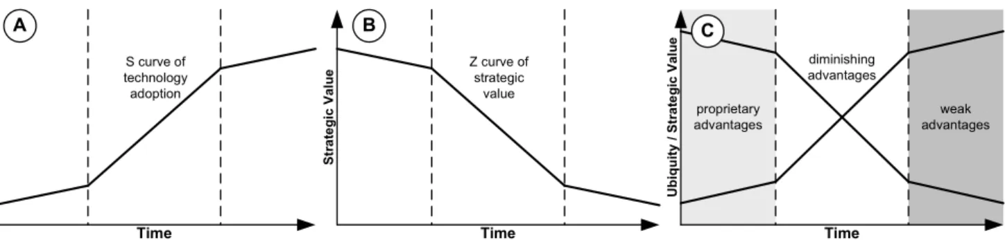
Generally, the adoption of information technology (IT) can be described by means of an S curve (cf. Fig. 1A) [19, 20, 74]. When new IT emerges, it is unproven, expensive, and difficult to use. Standards have not been established, and best practices still have to emerge. At this point, only

”first movers” start projects based on the emerging IT. They assume that the high costs and risks for being an innovator will be later compensated by gaining competitive advantage [18].

Picking up an emerging IT later, by contrast, allows to wait until it becomes more mature and standardized, resulting in lower introduction costs and risks. However, once the

∗supported by the Netherlands Organisation for Scientific Research (NWO), project 638.003.407, Value-based Business-IT Alignment (VITAL)

value of IT has become clear, both vendors and users rush to invest in it. Consequently, technical standards emerge and license costs decrease. Soon the IT is widely spread, with only few enterprises having not made respective investment decisions. The S curve is then complete.

Factors that typically push a new IT up the S curve in- clude standardization, price deflation, best practice diffu- sion, and consolidation of the vendor base. All these factors also erode the ability of IT as a mean for differentiation and competitive advantage. In fact, when dissemination of IT increases, its strategic potential shrinks at the same time.

Finally, once the IT has become part of the general infrastructure, it is typically difficult to achieve further strategic benefits (though rapid technological innovation often con- tinues). This can be illustrated by a Z curve (cf. Fig. 1B).

Considering the different curves of IT adoption, decisions about IT investments (and the appropriate moment of their introduction) constitute a difficult task to accomplish [17, 29] (cf. Fig. 1C). Respective decisions are influenced by numerous factors [42, 51, 53]. Hence, policy makers often demand for a business case [66] summarizing the key parameters of an IT investment. Thereby, different evaluation dimensions are typically taken into account [45]. As examples consider the costs of an investment, its assumed profit, its impact on work performance, business process performance, and the achievement of enterprise objectives.

In order to cope with different evaluation goals, numerous evaluation approaches have been introduced [61, 70, 71]. This survey gives an overview of existing evaluation approaches and discusses their suitability to deal with the complex economics of IT investments.

The remainder of this paper is organized as follows.

Section 2 introduces basic terminology related to IT evaluation. Section 3 introduces our framework for classifying and evaluating considered approaches. Section 4 deals with approaches for conducting evaluations from a financial viewpoint. Section 5 discusses methods for evaluating the impact of IT on business process and work performance. Fi- nally, Section 6 describes approaches for analyzing the impact of IT on enterprise objectives. Section 7 sums up and gives an overview of the discussed evaluation approaches.

(2)

Time

Ubiquity / Strategic Value

proprietary advantages

diminishing advantages

weak advantages

Time

Ubiquity

S curve of technology adoption

Time Strategic Value Z curve of

strategic value

A B C

Figure 1. The Curves of Technology Adoption.

Section 8 presents approaches that address value consider- ations without being conceived as evaluation approaches.

Section 9 gives an example showing how selected evaluation approaches can be used for evaluating IT. Section 10 concludes the survey with a summary.

2 Basic Terminology

Economic-driven IT evaluation typically focuses on the systematic analysis of related costs, benefits, and risks [55]

(though other aspects can be addressed as well). These terms are characterized in the following.

2.1 Costs

Generally, costs can be defined as the total expenses for goods or services including money, time and labor. Litera- ture distinguishes between different cost types [38]:

• Acquisition Costs: Refer to all costs which occur prior to an investment. This includes costs for purchasing an asset (e.g., an information system) as well as installa- tion costs.

• Historical Costs: Describe the total amount of money spent for an investment at purchase time or pay- ment. Historical costs are often listed in bookkeeping records. They are also denoted as accounting costs.

• Opportunity Costs: Denote the difference between the yield an investment earns and the yield which would have been earned if the costs for the investment had been placed into an alternative investment generating the highest yield available.

• Internal and External Costs: External costs occur out- side an organization and can be controlled by contracts and budgets. Internal cost, by contrast, occur within an organization (e.g., related to a specific project).

• Direct and Indirect Costs: Direct costs are associated with a particular cost factor, i.e., they can be budgeted.

Indirect costs, by contrast, cannot be budgeted, i.e., they cannot be represented with an explicit cost factor.

Figure 2. Different Types of Costs.

• Fixed and Variable Costs: Fixed costs do not vary, i.e., they do not alter during a given time-period. Variable costs, by contrast, may change [64].

• Life Cycle Cost: Refer to the costs of an investment over its entire life cycle. This includes costs for planning, research, development, production, maintenance, disposal, as well as cost of spares and repair times.

Considering this variety it seems hardly possible to introduce a standard meaning for the term ”costs”. Instead, ev- ery evaluation approach addressing costs has to carefully describe the assumed semantics in the given context.

2.2 Benefits

In economic-driven IT evaluations, costs are typically justified by expected benefits which are assumed to be gained through an IT investment. Generally, ”benefit” is a term used to indicate an advantage, profit, or gain attained by an individual or organization. Basically, two categories of benefits are distinguished [2, 35, 36]:

• Tangible Benefits: Tangible benefits are measurable and quantifiable [76]. Typically, monetary value can be assigned to tangible benefits. Regarding their quan- tification, one distinguishes between (i) increased rev- enues (i.e., resulting from increased revenues) and (ii) decreased costs (i.e., equating to cost savings).

(3)

• Intangible Benefits: Unlike tangible benefits, intan- gible benefits are typically not quantifiable. Instead, qualitative value (derived from subjective measures) is assigned to them [49]. As a typical example consider the impact of an investment on customer or employee satisfaction. Due to their complex quantification, intangible benefits are often not considered in a business case as they introduce a too great margin of error in economic calculations.

This categorization can be also observed when considering existing economic-driven IT evaluation approaches. While some evaluation approaches strictly focus on the quantification of tangible benefits [17, 70, 71], others consider intangible economic effects [36, 44, 59, 62].

2.3 Risks

Risk is the potential (positive or negative) impact of an investment that may arise from some present situation or some future event. It is often used synonymously with

”probability” and negative risk or threat. In professional risk assessments [7, 61], risk combines the probability of an event with the impact the event would have for an assumed risk scenario. In particular, financial risk is often consid- ered as the unexpected variability or volatility of revenues (which can be worse or better than expected). Note that risk-oriented evaluation approaches are not further considered in the context of this survey.

3 Comparing IT Evaluation Approaches

This section introduces the conceptual framework we use for classifying and comparing economic-driven IT evaluation approaches¹.

3.1 Existing Frameworks

In literature, there exist several frameworks that aim at comparing IT evaluation approaches:

• Andresen’s Framework [3]: This framework is based on nine criteria. Criterion 1 (extent of involvement) deals with the question which persons or user groups are affected when applying the evaluation approach.

Criterion 2 (stage of IT evaluation) concerns the ques- tion at which project stage an evaluation approach can be used. Criterion 3 (type of impact) addresses the ef- fects that can be analyzed with an evaluation approach.

Criterion 4 (costs of a method) deals with the effort re- lated to the use of an approach. Criterion 5 (number

1Note that software cost estimation approaches like Boehm’s constructive cost model (COCOMO) [11, 13] and Putnam’s software life cycle management (SLIM) [63] are not considered in this survey.

and type of evaluation) concerns the theoretical foun- dation of an evaluation approach. Criterion 6 (type of investment) deals with the question to what kind of IT investment an approach can be applied. Criterion 7 (scope of IT evaluation) concerns the enterprise level an approach is tailored to (e.g., management, opera- tional departments). Criterion 8 (difficulty) deals with the complexity related to the application of an evalu- ation approach. Finally, Criterion 9 (type of outcome) analyzes in which way evaluation results are presented.

• Pietsch’s Framework [60]: This framework utilizes ten criteria, many of them addressing the same or similar issues as Andresen’s criteria: theoretical foundation, evaluation object and scope, sources of evaluation data, stage of IT evaluation, flexibility, costs of an approach, tool support, transparency and traceability, completeness, and relevance for practice.

• Besides, there are enterprise architecture frameworks, e.g., Zachman’s framework [81] or the GRAAL frame- work [78, 80], which also address potential criteria for comparing IT evaluation approaches.

3.2 Our Framework

Though these frameworks address many important char- acteristics of IT evaluation approaches, they also neglect other basic issues. As examples consider the data needed for using an evaluation approach, the ability of an evaluation approach to allow for plausible conclusions, the objectiveness of an evaluation approach (and its resistance against manipulation), or the sensitivity of an evaluation approach when being confronted with an evolving information base- line (i.e., a varying data quality).

For these reasons, we have developed an adopted conceptual framework which combines criteria of the above frameworks with additional criteria derived from a profound literature study on economic-driven IT evaluation and practical needs we have identified in an empirical study [56].

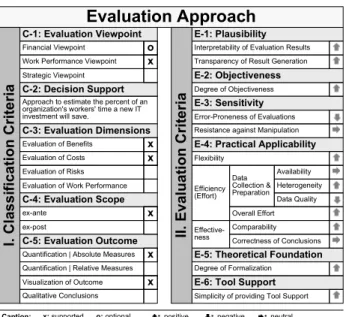
Fig. 3 shows our framework. Basic to this framework is the distinction between classification criteria and evalua- tion criteria. While the former allow for the categorization of approaches (based on identified similarities and differences), the latter enable us to analyze the general features of considered evaluation approaches.

3.2.1 Classification Criteria

This section summarizes criteria which can be used to classify IT evaluation approaches:

• Criterion C-1: Evaluation Viewpoint. We distinguish between three basic evaluation viewpoints. Ap-

(4)

Interpretability of Evaluation Results Transparency of Result Generation

Error-Proneness of Evaluations Resistance against Manipulation

Flexibility

Efficiency (Effort)

Effective- ness

Simplicity of providing Tool Support Degree of Objectiveness E-1: Plausibility

E-2: Objectiveness E-3: Sensitivity

E-4: Practical Applicability

E-6: Tool Support Data Collection &

Preparation Heterogeneity Availability

Data Quality

Correctness of Conclusions C-1: Evaluation Viewpoint

Strategic Viewpoint Financial Viewpoint Work Performance Viewpoint

C-2: Decision Support Approach to estimate the percent of an organization's workers' time a new IT investment will save.

Evaluation of Risks Evaluation of Benefits Evaluation of Costs

Evaluation of Work Performance C-3: Evaluation Dimensions

ex-post ex-ante

C-4: Evaluation Scope

Visualization of Outcome Quantification | Absolute Measures Quantification | Relative Measures

Qualitative Conclusions C-5: Evaluation Outcome

Comparability

Degree of Formalization

E-5: Theoretical Foundation Overall Effort

Caption:

Evaluation Approach

I. Classification Criteria II. Evaluation Criteria

x: supported o: optional :positive :negative :neutral

o x

x x

x

x x

Figure 3. The Criteria Framework at a Glance.

proaches for analyzing an IT investment from the fi- nancial viewpoint deal with the evaluation, distribu- tion, and consumption of financial value. Approaches for investigating IT investments from a work perfor- mance viewpoint evaluate the impact of an IT invest- ment on work performance and business process performance. Finally, approaches for conducting eval- uations from a strategic viewpoint allow to analyze the impact of an IT investment on the achievement of strategic enterprise objectives.

• Criterion C-2: Decision Support. It is the goal of most evaluation approaches to support decision making (e.g., investment decisions, project decisions, etc.) [46, 47]. Picking up this issue, we consider the suitability of an evaluation approach to support decisions as classification criterion.

• Criterion C-3: Evaluation Dimensions. This crite- rion deals with the evaluation dimension that can be analyzed by an evaluation approach. In our frame- work, we distinguish between the evaluation of costs, benefits, risks, and work performance.

• Criterion C-4: Evaluation Scope. We distinguish be- tween ex-ante and ex-post evaluations. Ex-ante eval- uations aim at the identification of the best solution in a given context. They focus on the economic feasibility of an investment, and they are typically con- ducted prior to an investment. However, they can also be used for evaluating an already initiated investment.

Note that the accuracy of ex-ante evaluations increases

with the number of available parameters (cf. Fig. 4).

Ex-post evaluations, by contrast, justify assumptions made during an ex-ante analysis, i.e., ex-post evaluations typically confirm or discard the results of a previous ex-ante evaluation.

Software Development Phases and Milestones Relative

Cost Range

x 4x

0,25x 1,25x 2x

0,85x

0,5x

Concept of Operation

Requirements Specifications

Product Design Specifications

Detailed Design Specifications

Accepted Software Feasibility Requirements Product

Design

Detailed Design

Development

& Test

Increasing Estimation Accuracy

Figure 4. Accuracy of Estimations.

• Criterion C-5: Evaluation Outcome. We distinguish between four types of evaluation outcome: (1) abso- lute figures (i.e., single numbers, calculated sums or differences), (2) relative figures (relating two absolute figures and analyzing their correlation), (3) graphical representations (i.e., tables, charts, and outlines for illustrating and visualizing both absolute and relative figures), and (4) textual evaluations.

These five criteria allow for the classification of IT evaluation approaches. Note that our discussions of specific evaluation approaches (Sections 4, 5 and 6) is organized along the three viewpoints of criterion C-1.

3.2.2 Evaluation Criteria

Before dealing with selected approaches in detail, we introduce criteria for evaluating the considered approaches.

Again, most evaluation criteria comprise sub criteria:

• Criterion E-1: Plausibility. This criterion deals with the ability of an evaluation approach to derive plausible results. Plausibility is determined by two sub crite- ria: (1) interpretability of results and (2) transparency of result generation. While the former addresses the clarity of evaluation results, the latter deals with the traceability of deriving an evaluation.

• Criterion E-2: Objectiveness. This criterion deals with the ability of an evaluation approach to produce the same or at least similar results when it is applied (to the same context) by different users. Approaches en- hancing a high degree of objectiveness exhibit fewer opportunities for manipulation.

(5)

Flexibility

Efficiency (Effort)

Effective- ness

Simplicity of providing Tool Support Degree of Objectiveness

E-1: Plausibility

E-6: Tool Support

Data Collection &

Preparation

Heterogeneity Availability

Data Quality

Correctness of Conclusions

C-1: Evaluation Viewpoint

C-2: Decision Support

Can be used to determine the profitability of an IT investment.

Evaluation of Work Performance

C-3: Evaluation Dimensions

ex-post ex-ante

Qualitative Conclusions

C-5: Evaluation Outcome

Comparability

E-5: Theoretical Foundation

Overall Effort

Return On Investment (ROI)

x

I. Classification Criteria

o x x

x x

x

II. Evaluation Criteria

Flexibility

Efficiency (Effort)

Effective- ness

E-1: Plausibility

E-6: Tool Support

Data Collection &

Preparation

Data Quality

Can be used to determine the period in which an IT investment’s costs amortize themselves.

ex-post ex-ante

Comparability

Overall Effort

Payback Period (PP)

x

o x x

x x

o x

A B

Caption: x: supported o: optional :positive :negative :neutral Caption: x: supported o: optional :positive :negative :neutral

Figure 5. Return on Investment and Payback Period.

• Criterion E-3: Sensitivity. This criterion concerns changes in evaluation results when underlying evaluation data is modified. High sensitivity means that small modifications of evaluation data can result in significant changes. Low sensitivity, in turn, implies that even strong modifications of evaluation data do not lead to strong changes. Thus, this criterion will be a measure for the error-proneness, if evaluation data is incomplete. Furthermore, this criterion also allows — like the previous criterion — to draw conclusions regarding the resistance of an evaluation approach against manipulation.

• Criterion E-4: Practical Applicability. Three sub cri- teria determine the practical applicability of an evaluation approach: (1) the ability of an evaluation approach to meet the varying requirements of different applica- tion domains (i.e., its flexibility), (2) the efforts for ac- complishing an evaluation (i.e., its efficiency), and (3) the ability of an evaluation approach to derive correct results (i.e., its effectiveness).

• Criterion E-5: Theoretical Foundation. Theoretical foundation enhances objectiveness.

• Criterion E-6: Tool Support. Tool support is an im- portant criterion as well.

4 Financial Viewpoint

This section discusses approaches that can be used to accomplish evaluations from a financial viewpoint (cf. Cri-

terion C-1). In particular, this viewpoint deals with the creation, distribution, consumption, and evaluation of economic value. It concerns the prediction of revenues and expenses based on the exchange of valuable goods and services between multiple actors. Evaluations from the financial viewpoint are typically based on traditional budgeting models and financial business ratios [61, 66]. These models and ratios consider the monetary costs and benefits of an investment over a specified period of time.

Thereby, we distinguish between static approaches (Sec- tion 4.1), dynamic approaches (Section 4.2), and cost- oriented approaches (Section 4.3). Note that the approaches discussed in the following can be used to analyze any economic investment.

4.1 Static Business Ratios

Static approaches ignore the time value of money. As ex- amples we consider return on investment, payback period, accounting rate of return, and break even analysis.

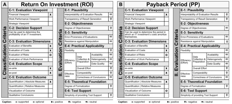
Return on Investment: Due to its simple calculation, re- turn on investment (ROI) has become one of the most popu- lar ratios to understand, evaluate and compare the economic value of different IT investment options. It measures the economic return of an investment, i.e., the effectiveness of using money to generate profit. More precisely, ROI describes how many times the net benefits of an investment (i.e., its benefits minus its initial and ongoing costs) cover the original investment:

(6)

Flexibility

Efficiency (Effort)

Effective- ness

E-1: Plausibility

E-6: Tool Support

Data Collection &

Preparation

Data Quality

Is a measure of profitability that associates the expected average return with the investment base.

C-3: Evaluation Dimension

ex-post ex-ante

Comparability

Overall Effort

Caption:

Accounting Rate Of Return (ARR)

x

o x x

x x

x

Flexibility

Efficiency (Effort)

Effective- ness

E-1: Plausibility

E-6: Tool Support

Data Collection &

Preparation

Data Quality

Is a parametric assessment of benefits, where the parameter values are selected to equate costs and benefits.

ex-post ex-ante

Comparability

Overall Effort

Caption:

Break Even Analysis

x

o x x

x x

o x

A B

Figure 6. Accounting Rate of Return and Break Even Analysis.

ROI =Bene f its−Costs

Costs *100%

There exist many variations of this definition [38] considering the multiple interpretations and applications in differ- ent industry domains, e.g., the return on invested capital (ROIC) or the financial ROI.

Fig. 5A shows the evaluation² of ROI based on our framework (cf. Section 3.2). Regarding the classification criteria (on the left side), ROI is an approach which can be related to the financial viewpoint (C-1). ROI takes into account both costs and benefits and — in certain variants — risks (C-3). Thereby, ROI supports both ex-ante and ex-post evaluations (C-4) and its result is an absolute measure (C- 5). Besides, the evaluation criteria (on the right side) allow to assess the ROI approach. Criterion E-1 in Fig. 5A, for example, expresses that the transparency of ROI result generation is easy to understand, while the interpretability of evaluation results can be considered neither as simple (i.e., positive) nor difficult (i.e., negative). Furthermore, the degree of objectiveness is high (E-2) and providing tool support is simple (E-6).

Payback Period: The payback period (cf. Fig. 5B) is the length of time required to compensate the original investment through its cash flows:

Payback Period = Cash f lowPerYear^Investment

It is assumed that the investment with earliest payback period is the best one. However, this is not always reasonable

2Note that in the following, we will not discuss these criteria in detail for the considered approaches.

for investments with large expected benefits in the future.

The payback period is a simple measure, but has its limi- tations. In particular, it neither address the time value of money nor does it consider anything else than the compen- sation of the initial investment. Fig. 5B shows the evaluation of the payback period approach based on our framework (cf. Section 3.2).

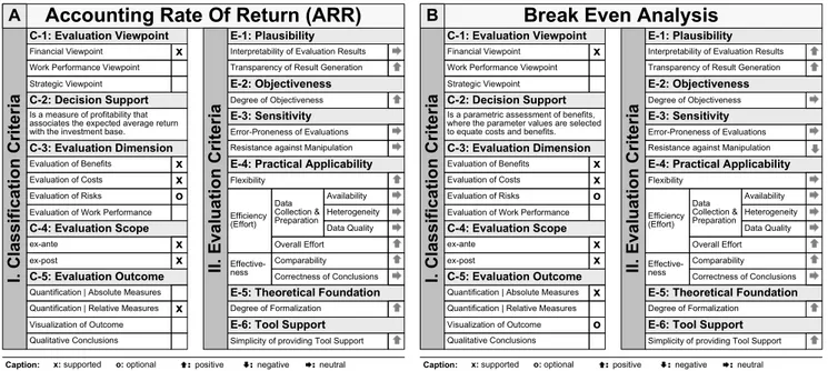
Accounting Rate of Return: The accounting rate of re- turn (cf. Fig. 5C) is a measure of profitability that associates the expected average return with the investment base. This ratio uses projected earnings based on financial statements rather than on cash flows:

Accounting Rate of Return =ExpectedAnnualEarnings AverageInvestment

”Expected Annual Earnings” denotes the expected annual income from the investment (or the average difference between revenues and expenses), and ”Average Investment” is the average or initial investment.

Break Even Analysis: The break even analysis (cf. Fig.

6B) is used when costs are quantifiable, but some key benefits are uncertain or intangible. It is particularly useful when the calculated break even level is ”extreme”, i.e., when it is outside the range of expected benefits.

4.2 Dynamic Business Ratios

Dynamic approaches consider the time value of money by comparing the initial cash outflows (or expenses) prior to

(7)

Flexibility

Efficiency (Effort)

Effective- ness

E-1: Plausibility

E-6: Tool Support

Data Collection &

Preparation

Data Quality

Discounted cash flow technique where all expected cash inflows and outflows are discounted to the present.

ex-post ex-ante

Comparability

Overall Effort

Caption:

Net Present Value (NPV)

x

o x x

x

Flexibility

Efficiency (Effort)

Effective- ness

E-1: Plausibility

E-6: Tool Support

Data Collection &

Preparation

Data Quality

The discount rate that makes an investment have a zero NPV

ex-post ex-ante

Comparability

Overall Effort

Caption:

Internal Rate of Return (IRR)

x

o x x

x

A B

Figure 7. Net Present Value and Internal Rate of Return.

an investment with the expected cash inflows (or revenues) of the investment. As examples consider net present value and internal rate of return.

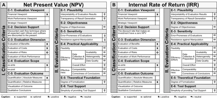
Net Present Value: The net present value (NPV) (cf. Fig.

7A) is a technique where all expected cash outflows and inflows are discounted to the present point in time. This is done by applying a discount rate to the difference of all expected inflows and outflows (the NPV is calculated from the current time t₀to some future point in time T ):

NPV =∑^T_i=0_(1+d)^Bⁱ^−Cⁱi

Thereby, Bi is the assumed benefit for the ith period in the future (i.e., the sum of the expected revenues), whereas Ci denotes the assumed costs for the same period (i.e., the sum of the expected outflows). ”d” is the discount factor.

The values of all expected inflows are added together, and all outflows are subtracted. The difference between the inflows and the outflows is the net present value. Generally, only investments with a positive NPV are acceptable as their return exceeds the discount rate.

Internal Rate of Return: As another example of a dy- namic budgeting model consider the internal rate of return (IRR) (cf. Fig. 7B). IRR is the annual rate at which an investment is estimated to pay off.

IRR and NPV are related though not equivalent. In particular, IRR does not use a discount rate. Instead, IRR takes into account the time value of money by considering the cash flows over the lifetime of an investment.

4.3 Cost-oriented Approaches

The approaches discussed in the following focus on the analysis and justification of IT investment costs: zero base budgeting approach, cost effectiveness analysis, target cost- ing approach, and total cost of ownership approach. Note that all these approaches go beyond the scope of the approaches discussed in Section 4.1 and Section 4.2.

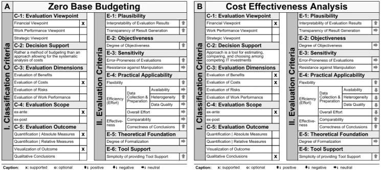
Zero Base Budgeting. The zero base budgeting approach (cf. Fig. 8A) is a budgeting method. It assumes that all costs of an investment have to be justified for each new period (e.g., a month, a quarter, a year), i.e., fundings are con- tinuously justified [60, 83].

Cost Effectiveness Analysis. Based on a cost effective- ness analysis (cf. Fig. 8B), one can compare and select the best out of several investment options [71]. A scoring model identifies key performance criteria for the candidate investments, assigns a score to each criterion, and finally computes a weighted overall score for each candidate investment. This requires the explicit identification, measure- ment and weighting of important decision factors based on subjective assessments.

Generally, cost effective analysis can be applied to different scenarios. A first scenario may be to minimize costs for a given level of effectiveness. As an example consider the choice among several printers. Each printer may be equally effective, and the issue is to choose the one with the lowest expected life cycle costs. A second scenario may be to maximize effectiveness for a given amount of costs. As an ex-

(8)

Flexibility

Efficiency (Effort)

Effective- ness

E-1: Plausibility

E-6: Tool Support

Data Collection &

Preparation

Data Quality

Rather a method of budgeting than an approach allowing for the systematic analysis of costs

ex-post ex-ante

Comparability

Overall Effort

Caption:

Zero Base Budgeting

x

x x

Flexibility

Efficiency (Effort)

Effective- ness

E-1: Plausibility

E-6: Tool Support

Data Collection &

Preparation

Data Quality

Approach is a tool for estimating, comparing, and choosing among competing IT investments

ex-post ex-ante

Comparability

Overall Effort

Caption:

Cost Effectiveness Analysis

x

x x

x

A B

Figure 8. Zero Base Budgeting and Cost Effectiveness Analysis.

ample consider the choice among several database management systems, where costs are identical, but features vary.

A final scenario may be to maximize effectiveness and minimize costs at the same time. As an example consider the selection of an engineering workstation where both performance features and costs might differ significantly.

This approach will be particularly useful if the benefits of an investment are quantifiable mainly in non-monetary dimensions. It does not allow for justifying an investment, i.e., it does not explicitly address the question whether the benefits of an investment exceed its costs.

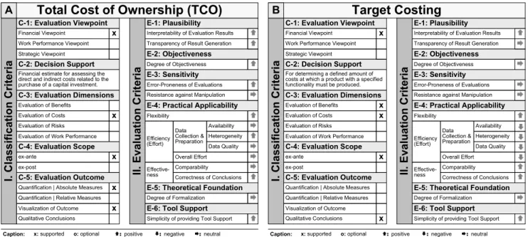
Total Cost of Ownership. The total cost of ownership (TCO) approach (cf. Fig. 9A) is a method to assess di- rect and indirect costs related to an investment [61]. A TCO assessment ideally results in a statement reflecting not only purchase costs, but also costs related to the future use and maintenance of the investment (as long as these costs can be made explicit). This includes costs caused by (planned and unplanned) failure or outage, costs for diminished performance incidents (i.e., if users are kept waiting), costs for security breaches (in loss of reputation and recovery costs), costs for disaster preparedness and recovery, floor space, electricity, development expenses, testing infrastructure and expenses, quality assurance, incremental growth, and de- commissioning. Often, TCO is used in financial analysis, e.g., ROI or IRR calculations, to quantify costs.

Target Costing. Target costing (cf. Fig. 9B) is a tech- nique for planning and realizing a defined amount of costs at which a product with a specified functionality has to be

produced to generate profitability [60, 73]. Besides, it also allows for identifying cost reductions by focusing on major ”design drivers” that influence costs. Therefore, target costing integrates strategic business and profit planning, competitive research and analysis, market research and customer requirements, research and development, technology advances, and product development. Target costing uses product portfolio profit plans to provide strategic summary schedules for product development, introduction and re- placement, or IT investments. Generally, target costing is different from a simple expenditure control mechanism as it aims at determining market-based prices for envelopes of features based upon market and competitive conditions in which price/volume relationships are examined.

5 Process Viewpoint

The process viewpoint focuses on the evaluation of oper- ational work and business process performance [37, 46, 47, 48, 57]. Characteristic to all approaches described in the following are quantifications based on information about process/work activities (e.g., start/completion times, average duration times, or waiting and idle times), process/work resources (e.g., resources needed, input and output data, or size of work queues), and quality metrics (e.g., failed or successful processes/work activities).

In the following, we describe four approaches: times savings times salary approach (Section 5.1), hedonic wage model (Section 5.2), activity-based costing (Section 5.3), and business process intelligence (Section 5.4).

(9)

Flexibility

Efficiency (Effort)

Effective- ness

E-1: Plausibility

E-6: Tool Support

Data Collection &

Preparation

Data Quality

Financial estimate for assessing the direct and indirect costs related to the purchase of a capital investment.

ex-post ex-ante

Comparability

Overall Effort

Caption:

Total Cost of Ownership (TCO)

x

x x

Flexibility

Efficiency (Effort)

Effective- ness

E-1: Plausibility

E-6: Tool Support

Data Collection &

Preparation

Data Quality

For determining a defined amount of costs at which a product with a specified functionality must be produced.

ex-post ex-ante

Comparability

Overall Effort

Caption:

Target Costing

x

x x

x

A B

Figure 9. Total Cost of Ownership and Target Costing.

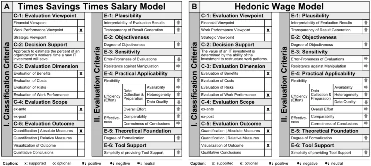
5.1 Times Savings Times Salary Approach The times savings times salary (TSTS) approach (cf. Fig.

13A) [70, 71] is based on the assumption that an employee’s salary is a measure of his ”contribution” or ”value” to an organization. Its goal is to estimate the work time an IT investment (e.g., a new information system) will save, and then to multiply that time with the salaries of all affected employees. For example, if an employee is currently devoting xj hours per week to activity aj, and if a new IT investment saves a total of Y% of his time, and if that saving includes yj hours in activity aj, then the change in the amount of time the employee will devote to activity aj can be calculated as follows [70]:

dx_j=Y(%)∗(xj−y_j)−y_j

The TSTS approach is based on five premises. First, it as- sumes that an employee’s value corresponds to his costs for an organization. Second, it assumes that saving x per- cent of an employee’s time is worth x percent of the em- ployee’s costs. Third, it is based on the assumption that the resources of an organization are efficiently allocated, i.e., that the costs of additional employees are balanced against their value for an organization. Consequently, the number of employees would not be higher even if it had been pos- sible to hire additional employees. Fourth, the TSTS ap- proach assumes that work comparable in value to current work remains to be done. In other words, it is assumed that there is additional work to which any saved time could be devoted, and that the value of work is comparable to work

currently done. Fifth, it assumes that saved time will be allocated among an employee’s productive activities.

The TSTS approach is easy to accomplish. As it is time-based, it can be used for evaluating the impact of IT on work performance and also on business process performance. However, there are three major problems derogating its use in practice. First, it is assumed that an employee’s value corresponds to his cost to an organization. This will be true if the organization is not resource-constrained and has hired the optimal number of employees. However, in general, the possibility that an employee’s value exceeds his costs should not be automatically dismissed. If his value is greater than his cost, then this approach will underesti- mate the true value of saved time. Second, and more im- portant, the TSTS approach does not take into account how the saved time is used. Instead, it is implicitly assumed that saved time is efficiently reallocated among available work activities. Consequently, it cannot be assumed that a partic- ular time allocation will take effect. Third, the calculation of the saved time implies that benefits are automatically re- alized. However, typically they are not, i.e., saved time may not result in economic benefit. The value of a new IT investment, for example, may be low or high, depending on how an organization and its flow of work is managed. The TSTS approach does not capture this variability.

5.2 Hedonic Wage Model

Like the TSTS approach, the hedonic wage model (cf.

Fig. 13B) [70] assumes that employees perform activities of different intrinsic value. The value of an IT investment,

(10)

in particular, is determined by its ability to restructure existing work patterns and to cause a shift in an employee’s work profile by replacing low-value-activities with tasks in a higher category. Such a restructuring can not only in- crease the efficiency (doing more of the same thing in the same amount of time) but also the effectiveness (doing more valuable work) of an organization and its employees.

The hedonic wage model assumes that employees carries out categories of activities (together making up his work profile). The aggregation of all work profiles into one work profile matrix (cf. Fig. 10) characterizes the work profile of an organization (with the level in the job hierarchy as the first dimension and the type of activity as the second one).

Note that both the number of job levels and activity types (i.e., the dimensions of the work profile matrix) are organization-specific, i.e., they may differ. In the example from Fig. 10, there exist five job levels (managers, spe- cialists, clerks, assistants, and secretaries) and six types of activities (management activity, specialist activity, routine activity, assistant activity, service activity, and other activity). Each value in Fig. 10 specifies how much time (in %) an employee (belonging to one of the five job levels) uses to conduct the six considered activities.

Wage per Hour

160€

120€

80€

60€

45€

Management Activity

(T1)

Specialist Activity

(T2) Routine Activity (T3)

Assistant Activity

(T4) Service Activity (T5)

Other Activity (T6) Manager (S1)

Specialist (S2) Clerk (S3) Assistant (S4) Secretary (S5)

53% 18% 23% 2% 2% 2%

13% 54% 13% 7% 2% 2%

5% 26% 17% 15% 7%

0% 0% 13% 55% 27% 5%

0% 0% 0% 15% 70% 15%

Type of Activity Level

in Job Hierarchy

18%

Each clerk utilizes (in average) 18% of his work time for specialist activities

Figure 10. Initial Work Profile Matrix.

From this matrix, a linear system of equations is derived (cf.

Fig. 11). Solving this system of equations (not shown here), it becomes possible to determine the value of the different activities [70]. In Fig. 11 a manager (job level S1), for example, has a value of 230.62$/h for the organization, but generates only costs of 160$ (his average wage per hour).

S1:0.50T1+0.15T2+0.20T3+0.05T4+0.05T5+0.05T6 = 160.00 €/h S2:0.10T1+0.60T2+0.10T3+0.10T4+0.05T5+0.05T6 = 120.00 €/h S3:0.02T1+0.15T2+0.35T3+0.20T4+0.18T5+0.10T6 = 80.00 €/h S4:0.00T1+0.00T2+0.10T3+0.55T4+0.30T5+0.05T6 = 60.00 €/h S5:0.00T1+0.00T2+0.00T3+0.15T4+0.70T5+0.15T6 = 45.00 €/h

230,62 $/h 130,55 $/h 96,93 $/h 63,87 $/h 50,60 $€/h Value

Linear System:

Figure 11. Linear System of Equations.

The value of an IT investment is derived based on a second work profile matrix. This second matrix reflects the (assumed) change in the work profile of an organization (caused by the investment). It is also converted into a linear system of equations which is then solved. The value of

the IT investment can be determined by comparing values of job levels before and after the investment.

Wage per Hour 160€

120€

80€

60€

45€

Management Activity

(T1)

Specialist Activity

(T2) Routine Activity (T3)

Assistant Activity

(T4) Service Activity (T5)

Other Activity (T6) Manager (S1)

Specialist (S2) Clerk (S3) Assistant (S4) Secretary (S5)

50% 15% 20% 5% 5% 5%

10% 60% 10% 10% 5% 5%

2% 15% 35% 20% 18% 10%

0% 0% 10% 55% 30% 5%

0% 0% 0% 15% 70% 15%

Type of Activity Level

in Job Hierarchy

Figure 12. Second Work Profile Matrix.

The hedonic wage model is similar to the TSTS approach, but avoids certain restrictive assumptions. For example, it produces more accurate value estimates. By estimating pre- and post-implementation work profile matrices, the projected values can be audited. However, disadvantages like the insufficient evaluation of qualitative factors remain.

5.3 Activity-based Costing

Activity-based costing (ABC) (cf. Fig. 15A) is a method of allocating costs to products and services. ABC helps to identify areas of high overhead costs per unit and therewith to find ways to reduce costs. Generally, ABC comprises the following steps:

• Step 1: The scope of the activities to be analyzed has to be identified (e.g., based on activity decomposition).

• Step 2: The identified activities are classified. Typi- cally, one distinguishes between value adding or non- value adding activities, between primary or secondary activities, and between required or non-required activ- ities. An activity will be considered as value-adding if the output of the activity is directly related to customer requirements, services or products (as opposed to ad- ministrative or logistical outcomes). Primary activities directly support the goals of an organization (whereas secondary activities support primary ones). Required activities are those that must always be performed.

• Step 3: Costs are gathered for those activities creat- ing the products or services of an organization. These costs can be related to salaries and expenditures for research, machinery, or office furniture.

• Step 4: Activities and costs are combined and the to- tal input cost for each activity is derived. This allows for calculating the total costs consumed by an activity.

However, at this stage, only costs are calculated. It is not yet determined where the costs originate from.

• Step 5: The ”activity unit cost” is calculated. Though activities may have multiple outputs, one output is