ARCTIC BIOMASS BURNING AEROSOL EVENT–

(1)

ARCTIC BIOMASS BURNING AEROSOL EVENT–

MICROPHYSICAL PROPERTY RETRIEVAL

Böckmann, Christine^1,*, Ritter, Christoph²and Ortiz-Amezcua, Pablo³

1University of Potsdam, Institute of Mathematics, Germany,^∗bockmann@uni-potsdam.de

2Alfred Wegener Institute for Polar and Marine Research, Germany

3University of Granada, Department of Applied Physics, Spain

ABSTRACT

An intense biomass-burning (BB) event from North America in July 2015 was observed over Ny-Ålesund (Spitsbergen, European Arc- tic). An extreme air pollution took place and aerosol optical depth (AOD) of more than 1 at 500nm occurs in middle and lower troposphere.

We analyse data from the multi-wavelength Raman-lidar KARL of Alfred Wegener Insti- tute to derive microphysical properties of the aerosol of one interesting layer from 3186 to 3306 m via regularization. We found credible and confidential microphysical parameters.

1 INTRODUCTION

The data for this work was obtained in Ny- Ålesund, Spitsbergen, in the European Arc- tic on 10 July 2015. An intensive event of BB aerosol originating from the boreal North America was observed for several days around that period at different Arctic sites (Markow- icz et al. [1]) and produced an AOD(500) >1.

Profiles of extinction and backscatter were obtained by the “3+2” Raman lidar KARL accord- ing to the method of Ansmann [2] with 10min / 30m resolution.

This event of BB aerosol and the KARL lidar are described also in [3]. The extinction and backscatter coefficient profiles are shown in Fig 1. For the inversion of the microphysics we selected an altitude range from 3186m to 3306m because a contemporaneous radiosonde showed a humidity about 80-85% and, hence, we expected a larger effective radius and a lower refractive index (RI) as was reported for dry BB aerosol in literature. Wandinger et al [4] derived for example effective radii of 0.25µm and RI of 1.56–1.66 for the real (Re)

and 0.05i–0.07i for the imaginary part (Im).

2 METHODOLOGY

The model relating the optical parametersΓ(λ) with the volume size distribution v(r) is described by the action of a Fredholm integral op- erator of the 1st kind with the kernel function K(r,λ;m) =_4r³Q(r,λ;m)and

Γ(λ) = rmax

rmin

K(r,λ;m)v(r)dr, (1) where λ is the wavelength, r is the radius, r_min, r_max are suitable lower and upper radius bounds,mis the complex RI,Γ(λ)denotes either the extinction or backscatter coefficients, and Q stands for either the extinction or the backscatter (dimensionless) Mie efficiencies respectively. The wavelength in our measurement cases can only take three discrete values 355, 532, and 1064 nm, since all the measurements were performed with the Raman lidar forming data sets of 3 backscatter coefficients in all three wavelengths and 2 extinction coefficients in the first two. Identifying Γ(λ) as our measurement data andv(r)as the unknown volume distribution, the problem reduces to the inversion of Eq. (1). Knowing the volume distribution, we can then extract the following microphysical parameters

•total surface-area concentration (µm²cm⁻³) s_t=3 ^v(r)_r dr

•total volume concentration (µm³cm⁻³) v_t=v(r)dr

•total number concentration (cm⁻³) n_t=3/4π ^v(r)_r3 dr

•effective radius (µm) r_eff=3^v_s^t

t.

In addition, the complex RI and the single scat- tering albedo (SSA) in 355 nm and 532 nm are retrieved. Note, that in this work the com-

EPJ Web of Conferences 176, 05023 (2018) https://doi.org/10.1051/epjconf/201817605023 ILRC 28

(2)

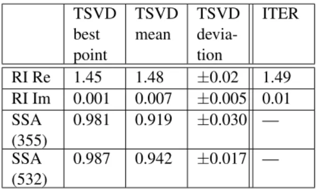
Table 1:Retrieved RI and SSA using both methods.

TSVD best point

TSVD mean

TSVD deviation

ITER

RI Re 1.45 1.48 ±0.02 1.49 RI Im 0.001 0.007 ±0.005 0.01 SSA

(355)

0.981 0.919 ±0.030 — SSA

(532)

0.987 0.942 ±0.017 —

mon assumption of wavelength-independent RI is made, as a member of the predefined grid in- troduced, see e.g. [5, 6, 7]. Solving Eq. (1) requires discretization, regularization and a parameter choice rule, see e.g. [5, 8].

2.1 TSVD regularization

We discretized Eq. (1) with spline collocation.

The volume distribution v(r) is approximated with respect to the B-spline functions φj by vn=∑ⁿ_j=1bjφj, reducing the problem to the de- termination of the coefficientsb_j. The contin- uous problem (Eq. (1)) is now replaced by a discrete oneAb=Γ, where the matrix elements of the linear system are

Ai j=_r^r_min^maxK(λ_i,r;m)φj(r)dr (2) andΓ is a vector now. By doing so, we have already projected our problem to a finite n- dimensional space. Clearly, the decision about the projected dimension (n) and order (d) of the base functionsφ_j is critical, since an appropriate representation of our solution strongly de- pends on it. This is not done at once; on the contrary, the algorithm constructs a linear system (5×n) for each value ofnandd specified and every RI within our predefined grid. For example, we first fix the refractive index, and calculate the kernel functions, then decide for candidates for n and d, e.g., n=3, . . . ,8 and d=3,4 which define a B-spline function and finally calculate the matrix elements from Eq.

(2). For more particular details on the B-spline basis in the frame of a non-negative size distribution, we are looking for, see [5].

Each linear system is solved by first expanding the matrix using Singular Value Decomposition (SVD). Potential noise in our matrix will be magnified as a result of the singular values clus- tering to zero. We would like to prevent this be- havior by including only a part of the SVD, i.e defining a certain cut-off level k, above which the most noisy solution coefficients are filtered out. This regularization procedure is known as Truncated SVD (TSVD), see [5].The parameter choice rule consists in selecting an appropriate triple(n,d,k)heuristically.

2.2 Iterative regularization

A particular iterative regularization (ITER) was used additionally to retrieve microphysical properties of this event. This method is based on Runge-Kutta regularization, see [8, 9]. Since the noise level of the backscatter and extinction profile is often not known or only a roughly estimation is available, a heuristical parameter choice rule is used here too, the well-known L- curve method. This method was developed to retrieve the fine mode only until 1.25µm.

3 RESULTS

The retrieval by TSVD was first done with a refractive index grid with a resolution of 40x40 points and a range for the Re of RI from 1.3- 1.8 and for the Im from 0-0.05. We found that the best possible RI’s lay on a diagonal pattern what is an indication of precise measurements in agreement with investigated simulations, see [10]. The best points are situated in the range 1.4-1.55 for Re and 0-0.025 for Im. There- fore, the retrieval was done a second time on those ranges with a grid resolution of 20x20, see Fig. 2 (top). We selected the 12 points with a relative residual norm below 8% and a similar shape of the volume distribution. The best point (7.22%) was found for m=1.45+0.00132i.

Averaging all 12 selected RI points results in m=1.48+0.00713i, see Table 1. Addition- ally, the second algorithm ITER found a similar value m=1.49+0.01iwhich is in accor-

2

(3)

Table 1:Retrieved RI and SSA using both methods.

TSVD best point

TSVD mean

TSVD deviation

ITER

RI Re 1.45 1.48 ±0.02 1.49 RI Im 0.001 0.007 ±0.005 0.01 SSA

(355)

0.981 0.919 ±0.030 — SSA

(532)

0.987 0.942 ±0.017 —

mon assumption of wavelength-independent RI is made, as a member of the predefined grid in- troduced, see e.g. [5, 6, 7]. Solving Eq. (1) requires discretization, regularization and a parameter choice rule, see e.g. [5, 8].

2.1 TSVD regularization

We discretized Eq. (1) with spline collocation.

The volume distribution v(r) is approximated with respect to the B-spline functions φj by vn=∑ⁿ_j=1bjφj, reducing the problem to the de- termination of the coefficientsb_j. The contin- uous problem (Eq. (1)) is now replaced by a discrete oneAb=Γ, where the matrix elements of the linear system are

Ai j=_r^r_min^maxK(λ_i,r;m)φj(r)dr (2)

andΓ is a vector now. By doing so, we have already projected our problem to a finite n- dimensional space. Clearly, the decision about the projected dimension (n) and order (d) of the base functionsφ_j is critical, since an appropriate representation of our solution strongly de- pends on it. This is not done at once; on the contrary, the algorithm constructs a linear system (5×n) for each value ofnandd specified and every RI within our predefined grid. For example, we first fix the refractive index, and calculate the kernel functions, then decide for candidates for n and d, e.g., n=3, . . . ,8 and d=3,4 which define a B-spline function and finally calculate the matrix elements from Eq.

(2). For more particular details on the B-spline basis in the frame of a non-negative size distribution, we are looking for, see [5].

Each linear system is solved by first expanding the matrix using Singular Value Decomposition (SVD). Potential noise in our matrix will be magnified as a result of the singular values clus- tering to zero. We would like to prevent this be- havior by including only a part of the SVD, i.e defining a certain cut-off level k, above which the most noisy solution coefficients are filtered out. This regularization procedure is known as Truncated SVD (TSVD), see [5].The parameter choice rule consists in selecting an appropriate triple(n,d,k)heuristically.

2.2 Iterative regularization

A particular iterative regularization (ITER) was used additionally to retrieve microphysical properties of this event. This method is based on Runge-Kutta regularization, see [8, 9]. Since the noise level of the backscatter and extinction profile is often not known or only a roughly estimation is available, a heuristical parameter choice rule is used here too, the well-known L- curve method. This method was developed to retrieve the fine mode only until 1.25µm.

3 RESULTS

The retrieval by TSVD was first done with a refractive index grid with a resolution of 40x40 points and a range for the Re of RI from 1.3- 1.8 and for the Im from 0-0.05. We found that the best possible RI’s lay on a diagonal pattern what is an indication of precise measurements in agreement with investigated simulations, see [10]. The best points are situated in the range 1.4-1.55 for Re and 0-0.025 for Im. There- fore, the retrieval was done a second time on those ranges with a grid resolution of 20x20, see Fig. 2 (top). We selected the 12 points with a relative residual norm below 8% and a similar shape of the volume distribution. The best point (7.22%) was found for m=1.45+0.00132i.

Averaging all 12 selected RI points results in m=1.48+0.00713i, see Table 1. Addition- ally, the second algorithm ITER found a similar value m=1.49+0.01iwhich is in accor-

Figure 1:Optical backscatter and extinction coefficient profiles from Raman lidar KARL and aerosol layer of

interest (dotted horizontal lines).

Figure 2:Top: Retrieved complex refractive index grid.

Bottom: 12 retrieved volume distributions (thin black lines) and mean distribution (thick blue line).

dance with the deviation level from the first algorithm, see Table 1. Comparing both algorithms for the used B-spline bases yields: Both

Figure 3:Retrieved volume distribution of the best point, see Fig. 2 with TSVD and two log-normal modes

for fine and coarse mode (green lines).

Table 2:Retrieved microphysical properties of the inverted and fitted distributions. Values in brackets stand

for: (.) best point and {.} used r_min=0.125µm (regular used rmin=0.001µm ).

mean TSVD

fine mode

coarse mode

r_med — 0.19

(0.22)

1.60 (1.11)

σ — 1.71

(1.63)

1.08 (1.24) r_eff 0.45

±0.01 (0.46)

0.40

——

(0.39)

1.63

——

(1.24)

v_t 83.7

±2.24 (87.0)

66.3

——

(59.2)

6.1

——- (24.02)

s_t 561

±2.5 (564)

501

——

(454)

11.25

——

(58.2)

nt {477}

({479})

602 (478)

0.35 (3.5) determined for all selected distributionsn=8 (only two outliers n=7,9) and d =3 for the number and degree of the used splines, respectively. Moreover, with respect to TSVD no ad- ditional cut of any singular value was neces- sary. The retrieved mean volume distribution, see Fig. 2 bottom (blue line), and in particular the best point distribution shows obviously a bi-modal volume distribution, one for the fine mode and one for the coarse mode particles. It is commonly assumed that the number distribution is a log-normal distribution, this property is also true for the surface-area and the volume

3

(4)

distribution with the same geometric standard deviation as well. Therefore, we separated the distribution into two modes by using two log- normal distributions such that the sum of both modes (brown line) fits the retrieved volume distribution well, see Fig. 3. Finally, we sum- marized all microphysical parameters in Table 2 for the whole distribution as well as for the two modes separately. We remark, that for the total number concentration of the complete mean distribution the Aitken-mode (first part of the fine mode) was excluded since even very small uncertainties in the volume distribution by di- viding byr³with very small radii lead to a huge amplification.

4 CONCLUSIONS

We found for the effective radius of the complete mean distributionreff=0.45±0.01µm as well as for the fine and coarse mode 0.40µm and 1.24µm, respectively. Our expectation was approved. Because of the large humidity 80- 85% in the regarded particle layer, the effective radius of the BB-particles is larger as usual in the literature, e.g. 0.25µm in [4]. Furthermore, in agreement the RI is indeed lower in both parts for such wet particles, compare the Intro- duction last part and Table 1. Analyzing the whole profile is an ongoing work but some of the particle properties between 2km and 3.3km altitude are also discussed in [3].

ACKNOWLEDGEMENTS

The work has been supported partially by the European Union (EU) Seventh Framework Program for research, technological development and demonstration under grant agreement No. 289923 - ITaRS and EU’s Horizon 2020 research and innovation programme under grant agreement No. 654109 (ACTRIS-2). This work was also partially funded by the Spanish Ministry of Education, Cul- ture and Sports through grant FPU14/03684 with the sup- port of the Erasmus+ programme of the EU.

References

[1] Markowicz, K.M., Pakszys, P., Ritter, C., Zielin- ski, T., Udisti, R., Cappelletti, D., Mazzola, M., Shiobara, M., Lynch, P., Zawadzka, O., Lisok,

J., Petelski, T., Makuch, P., Karasinski, G.:

2016, Impact of North American intensive fires on aerosol optical properties measured over the Euro- pean Arctic in July 2015, accepted at JGR, doi:

10.1002/2016JD025310.

[2] Ansmann, A., Wandinger, U., Riebesell, M., Weitkamp, C., and Michaelis, W. 1992: Indepen- dent measurement of extinction and backscatter profiles in cirrus clouds by using a combined Raman elastic-backscatter lidar, Appl. Opt. 31, 7113-7113.

[3] Ritter, C. and Böckmann, C.: Observation of an intensive Biomass Burning Event over Spitsbergen (this issue).

[4] Wandinger, U., Müller, D., Böckmann, C., Al- thausen, D., Matthias, V., Bösenberg, J., ... and Ansmann, A. (2002). Special Section: Lindenberg Aerosol Chracterization Experiments (LACE): LAC 7 Optical and microphysical characterization of biomass-burning and industrial-pollution aerosols from multiwavelength lidar. Journal of Geophys- ical Research-Part D-Atmospheres, 107(21), doi:

10.1029/2000JD000202.

[5] Böckmann, C., 2001: Hybrid regularization method for the ill-posed inversion of multiwavelength lidar data to determine aerosol size distributions, Appl.

Opt.40, 1329–1342.

[6] Kirsche, A., 2003: Entwicklung der Runge-Kutta Iteration und Anwendung als Regularisierungsver- fahren,Diploma thesis University of Potsdam.

[7] Samaras, S., Nicolae, D., Böckmann, C., Vasilescu, J., Binietoglou, J., Labzovskii, L., Toanca, F., and Papayannis, A., 2015: Using Raman-lidar-based regularized microphysical retrievals and Aerosol Mass Spectrometer measurements for the characterization of biomass burning aerosols,J. Comput.

Phys.299, 156–174.

[8] Böckmann, C. and Kirsche, A., 2006: Iterative regularization method for lidar remote sensing,Comput.

Phys. Commun.174, 607–615.

[9] Osterloh, L., Pérez, C., Böhme, D., Baldasano, J. M., Böckmann, C., Schneidenbach, L., and Vi- cente, D., 2009: Parallel software for retrieval of aerosol distribution from LIDAR data in the framework of EARLINET-ASOS,Comput. Phys. Com- mun.180, 2095–2102.

[10] Müller, D., Böckmann, C., Kolgotin, A., Schnei- denbach, L., Chemyakin, E., Rosemann, J., Znak, P., and Romanov, A., 2016: Microphysical particle properties derived from inversion algorithms developed in the framework of EARLINET,Atmos. Meas.

Tech.9, 5007–5035.

4