Convergence Rate of Runge–Kutta-Type Regularization for Nonlinear Ill-Posed Problems under Logarithmic Source Condition

Article

Convergence Rate of Runge–Kutta-Type Regularization for Nonlinear Ill-Posed Problems under Logarithmic Source Condition

Pornsarp Pornsawad^1,2, Elena Resmerita^3,* and Christine Böckmann^4,5

Citation: Pornsawad, P.; Resmerita, E.; Böckmann, C. Convergence Rate of Runge–Kutta-Type Regularization for Nonlinear Ill-Posed Problems under Logarithmic Source Condition.Mathematics2021,9, 1042.

https://doi.org/10.3390/math9091042

Academic Editor: Denis N. Sidorov

Received: 12 March 2021 Accepted: 1 May 2021 Published: 4 May 2021

Publisher’s Note:MDPI stays neutral with regard to jurisdictional claims in published maps and institutional affil- iations.

Copyright: © 2021 by the authors.

Licensee MDPI, Basel, Switzerland.

This article is an open access article distributed under the terms and conditions of the Creative Commons Attribution (CC BY) license (https://

creativecommons.org/licenses/by/

4.0/).

1 Department of Mathematics, Faculty of Science, Silpakorn University, 6 Rachamakka Nai Rd., Nakhon Pathom 73000, Thailand; pornsawad_p@silpakorn.edu

2 Centre of Excellence in Mathematics, Mahidol University, Rama 6 Rd., Bangkok 10400, Thailand

3 Institute of Mathematics, Alpen-Adria University of Klagenfurt, Universitätsstr. 65-67, A-9020 Klagenfurt, Austria

4 Institute of Mathematics, University of Potsdam, Karl-Liebknecht-Str. 24-25, 14476 Potsdam, Germany;

bockmann@uni-potsdam.de

5 Helmholtz Centre for Polar and Marine Research, Alfred Wegener Institute, Telegrafenberg A45, 14473 Potsdam, Germany

* Correspondence: elena.resmerita@aau.at

Abstract:We prove the logarithmic convergence rate of the families of usual and modified iterative Runge–Kutta methods for nonlinear ill-posed problems between Hilbert spaces under the logarith- mic source condition, and numerically verify the obtained results. The iterative regularization is terminated by the a posteriori discrepancy principle.

Keywords: nonlinear inverse problem; ill-posed problem; iterative regularization; Runge–Kutta methods; logarithmic source condition; discrepancy principle; convergence rate

1. Introduction

LetXandYbe infinite-dimensional real Hilbert spaces with inner productsh·,·iand normsk · k. Let us consider a nonlinear ill-posed operator equation

F(w) =g, (1)

whereF:D(F)⊂X→Yis a nonlinear operator between the Hilbert spacesXandY. We assume that (1) has a solutionw⁺for exact data (which need not be unique). We have approximate datag^εwith

kg^ε−gk ≤ε, ε>0. (2) Besides the classical Tikhonov–Phillips regularization, a plethora of interesting variational and iterative approaches for ill-posed problems can be found, e.g., in Morozov [1], Tikhonov and Arsenin [2], Bakushinsky and Kokurin [3], and Kaltenbacher et al. [4]. We focus here on iterative methods, as they are also very popular and effective to use in applications.

The simplest iterative regularization is the Landweber method—see, e.g., Hanke et al. [5], where the analysis for convergence rates is done under Hölder-type source condition. A more effective method often used in applications is the Levenberg–Marquardt method

w^ε_k+1=w^ε_k+ (α_kI+F⁰(w^ε_k)^∗F⁰(w^ε_k))⁻¹F⁰(w^ε_k)^∗(g^ε−F(w^ε_k)). (3) This was investigated in [6–8] under the Hölder-type source condition (HSC) and a posteriori discrepancy principle (DP). Jin [7] proved optimal convergence rates for an a priori chosen geometric step size sequenceα_k, whereas Hochbruck and Hönig [6] showed convergence with the optimal rate for quite general step size sequences including the

Mathematics2021,9, 1042. https://doi.org/10.3390/math9091042 https://www.mdpi.com/journal/mathematics

geometric sequence. Later, Hanke [8] avoided any constraints on the rate of decay of the regularization parameter to show the optimal convergence rate.

Tautenhahn [9] proved that asymptotic regularization, i.e., the approximation of problem (1) by a solution of the Showalter differential equation (SDE)

d

dtw^ε(t) =F⁰(w^ε(t))^∗[g^ε−F(w^ε(t))], 0<t≤T, w^ε(0) =w,¯ (4) where the regularization parameterTis chosen according to the DP under the HSC, is a stable method to solve nonlinear ill-posed problems.

Solving SDE by the family of Runge–Kutta (RK) methods delivers a family of RK-type iterative regularization methods

w^ε_k+1=w^ε_k+τ_kb^T(δ+τ_kAF⁰(w^ε_k)^∗F⁰(w^ε_k))⁻¹_1F⁰(w^ε_k)^∗(g^ε−F(w_k^ε)), k∈N0, (5) where1denotes the(s×1)vector of identity operators, whileδis the (s×s)diagonal matrix of bounded linear operators with identity operator on the entire diagonal and zero operator outside of the main diagonal with respect to the appropriate spaces. The parameter τ_k=1/α_kin (5) is the step-length, also called the relaxation parameter. The(s×s)matrix Aand the(s×1)vectorbare the given parameters that correspond to the specific RK method, building the so-called Butcher tableau (succession of stages). Different choices of the RK parameters generate various iterative methods.

Böckmann and Pornsawad [10] showed convergence for the whole RK-type family (including the well-known Landweber and the Levenberg–Marquardt methods). That paper also emphasized advantages of using some procedures from the mentioned family, e.g., regarding implicit A-stable Butcher tableaux. For instance, the Landweber method needs a lot of iteration steps, while those implicit methods need only a few iteration steps, thus minimizing the rounding errors.

Later, Pornsawad and Böckmann [11] filled in the missing results on optimal conver- gence rates, but only for particular first-stage methods under HSC and using DP.

Our current study considers further the unifying RK-framework described above, as well as a modified version presented below, showing optimality of the RK-regularization schemes under logarithmic source conditions.

An additional termα_k(w^ε_k−ξ), as in the iteratively regularized Gauss–Newton method (see, e.g., [4]),

w^ε_k+1=w^ε_k−(F⁰(w^ε_k)^∗F⁰(w^δ_k) +α_kI)⁻¹(F⁰(w^ε_k)^∗(F(w^ε_k)−g^ε) +α_k(w^ε_k−ξ)), was added to a modified Landweber method. Thus, Scherzer [12] proved a convergence rate result under HSC without particular assumptions on the nonlinearity of operator F. Moreover, in Pornsawad and Böckmann [13], an the additional term was included to the whole family of iterative RK-type methods (which contains the modified Landweber iteration),

w^ε_k+1=w^ε_k+τ_kb^TΠ⁻¹1F⁰(w^ε_k)^∗(g^ε−F(w^ε_k))−τ_k⁻¹(w^ε_k−ζ)_{, (6)} whereζ ∈ XandΠ = δ+τ_kAF⁰(w^ε_k)^∗F⁰(w^ε_k). Using a priori and a posteriori stopping rules, the convergence rate results of the RK-type family are obtained under HSC if the Fréchet derivative is properly scaled.

Due to the minimal assumptions for the convergence analysis of the modified iterative RK-type methods, an additional term was added to SDE

d

dtw^ε(t) =F⁰(w^ε(t))^∗[g^ε−F(w^ε(t))]−(w^ε(t)−w¯)_{, 0}<t≤T, w^ε(₀) =w.¯ (7) Pornsawad et al. [14] investigated this continuous version of the modified iterative RK-type methods for nonlinear inverse ill-posed problems. The convergence analysis yields the optimal rate of convergence under a modified DP and an exponential source condition.

Recently, a second-order asymptotic regularization for the linear problem ˆAx=ywas investigated in [15]

¨

x(t) +µx˙(t) +A^ˆ∗Axˆ (t) =A^ˆ∗y^δ,x(0) =x, ˙¯ x(0) =x˙¯

under HSC using DP.

Define

ϕ=ϕp, ϕp(λ):=

( ln_λ^e−p

for 0<λ≤1

0 forλ=0 (8)

withp>0 and the usual logarithmic sourcewise representation

w⁺−w₀=ϕ F⁰(w⁺)^∗F⁰(w⁺)v, v∈X, (9) wherekvkis sufficiently small andw0∈ D(F)is an initial guess that may incorporate a priori knowledge on the solution.

In numerous applications—e.g., heat conduction, scattering theory, which are severely ill- posed problems—the Hölder source condition is far too strong. Therefore, Hohage [16] proved convergence and logarithmic convergence rates for the iteratively regularized Gauss–Newton method in a Hilbert space setting, provided a logarithmic source condition (9) is satisfied and DP is used as the stopping rule. Deuflhard et al. [17] showed some convergence rate result for the Landweber iteration using DP and (9) under a Newton–Mysovskii condition on the nonlinear operator. Sufficient conditions for the convergence rate, which is logarithmic in the data noise level, are given.

In Hohage [18], a systematic study of convergence rates for regularization methods under (9) including the case of operator approximations for a priori and a posteriori stopping rules is provided. A logarithmic source condition is considered by Pereverzyev et al. [19] for a derivative-free method, by Mahale and Nair [20] for a simplified generalized Gauss–

Newton method, and by Böckmann et al. [21] for the Levenberg–Marquardt method using DP as stopping rule. Pornsawad et al. [22] solved the inverse potential problem, which is exponentially ill-posed, employing the modified Landweber method and proved convergence rate under the logarithmic source condition via DP for this method.

To the best of our knowledge, for the first time, convergence rates are established both for the whole family of RK-methods and for the modified version, when applied to severely ill-posed problems (i.e., under the logarithmic source condition).

The structure of this article is as follows. Section2provides assumptions and technical estimations. We derive the convergence rate of the RK-type method (5) in Section3and of the modified RK-type method (6) in Section4under the logarithmic source conditions (8) and (9). In Section5, the performed numerical experiments confirm the theoretical results.

2. Preliminary Results

Lemma 1. Let K be a linear operator withkKk ≤1. For k∈N with k>1,e0:= ϕ(λ)v withϕ given by (8) and p>0, there exist positive constants c1and c2such that

(I−K^∗K)^ke0

≤c1(ln(k+e))^−pkvk (10) and

K(I−K^∗K)^ke₀

≤c₂(k+1)^−1/2(ln(k+e))^−pkvk. (11) Proof. By spectral theory (8), and (A1) and (A2) in [22], we have

(I−K^∗K)^ke0

≤ k(I−K^∗K)^kϕ(K^∗K)kkvk

≤ sup

λ∈(0,1]

|(1−λ)^k(1−lnλ)^−p|kvk

≤ c1(ln(k+e))^−pkvk, (12) for some constantc₁>0. Similarly, spectral theory (8), and (A3) and (A4) in [22], provides

K(I−K^∗K)^ke0

≤ k(I−K^∗K)^k(K^∗K)^1/2ϕ(K^∗K)kkvk

≤ sup

λ∈(0,1]

|(1−λ)^kλ^1/2(1−lnλ)^−p|kvk

≤ c2(k+1)^−1/2(ln(k+e))^−pkvk, (13) for some constantc2>0.

Assumption 1. There exist positive constants cL,cr, andbcRand a linear bounded operator Rw: Y→Y such that for w∈Bρ(w0), the following conditions hold

F⁰(w) =RwF⁰(w⁺) (14) kRw−Ik ≤cL

w−w⁺

(15)

kRwk ≤cr (16)

|kRwk − kIk| ≥_bcR, (17) where w⁺is the exact solution of(1).

Lete_k:=w⁺−w^ε_kbe the error of thekth iterationw^ε_k,S_k :=F⁰(w^ε_k)_andS:=F⁰(w⁺)_. Proposition 1. Let the conditions(14)and(15)in Assumption1hold. Then,

F(w^ε_k)−F(w⁺)−F⁰(w⁺)(w^ε_k−w⁺)≤ ¹

2cLke_kkkSe_kk (18) for w∈B_ρ(w₀).

The proof is given in [22] using the mean value theorem.

Assumption 2. Let K be a linear operator and τ be a positive number. There exist positive constants D1and D2such that

kI−τf(−τKK^∗)k ≤ D₁ (19) and

kI+τf(−τKK^∗)k ≤D₂, (20) with f(t):=b^T(I−At)⁻¹1.

We note that the explicit Euler method provideskI−τf(−τKK^∗)k ≤ |1−τ|and kI+τf(−τKK^∗)k ≤ |1+τ|. Thus, the conditions (19) and (20) hold if τ is bounded.

For the implicit Euler method, we have

kI−τf(−τKK^∗)k ≤ sup

0<λ≤λ0

|1−τ(1+τλ)⁻¹| and

kI+τf(−τKK^∗)k ≤ sup

0<λ≤λ₀

|1+τ(1+τλ)⁻¹|,

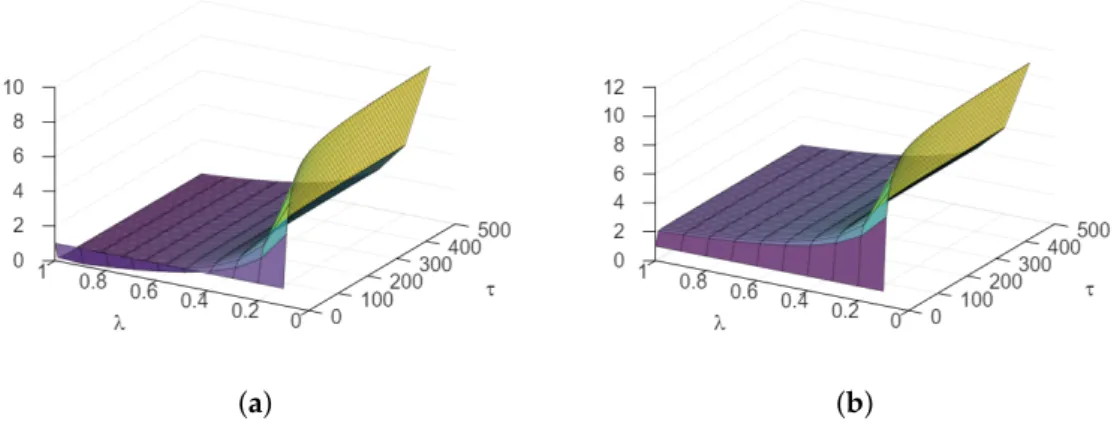
for some positive numberλ₀. We observe from Figure1that the conditions (19) and (20) hold forτ>0.

(a) (b)

Figure 1. Plots of (a)z = |1−τ(1+τλ)⁻¹|and (b)z = |1+τ(1+τλ)⁻¹|for 0 < λ ≤ 1 and 0<τ≤500.

Finally, we need a technical result for the next two sections.

Lemma 2. Let Assumptions1and2hold for the operator S := F⁰(w⁺). Then, there exists a positive number cRsuch that

i) kI−τ_kR^∗_wε

kf(−τ_kSkS^∗_k)k ≤cRkw⁺−w^ε_kk (21)

and

ii) k(1−α_k)I−τ_kR^∗_wε

kf(−τ_kS_kS^∗_k)k ≤c_Rkw⁺−w^ε_kk. (22) Proof. (i) Following the proof technique of Theorem 1 in [22] and using (17), we have

1≤_bc⁻¹_R kRw−Ik (23)

and

kI+R^∗_wk ≤_bc⁻¹_R kI−R^∗_wkkI+R^∗_wk. (24) Using Assumption2; the estimates in Equations (15), (16), (19), (20), (24); and the triangle inequality, we obtain

kI−τ_kR^∗_wε

kf(−τ_kS_kS^∗_k)k

= 1 2

h(I+R^∗_wε

k)(I−τ_kf(−τ_kS_kS^∗_k))ⁱ+¹ 2

h(I−R^∗_wε

k)(I+τ_kf(−τ_kS_kS^∗_k))ⁱ

≤¹

2kI+R^∗_wε

kkkI−τ_kf(−τ_kSkS^∗_k)k+¹

2kI−R^∗_wε

kkkI+τ_kf(−τ_kSkS^∗_k)k

≤¹ 2 h

bc⁻¹_R D1kI+R^∗_wε kk+D2

ikI−R^∗_wε kk

≤cRkw⁺−w^ε_kk, (25)

with positive numbercR= ¹₂^h_bc⁻¹_R D₁(kIk+cr) +D2

icL. (ii) DenoteA_k=τ_kR^∗_wε

kf(−τ_kS_kS^∗_k). We have k(1−α_k)I−A_kk ≤ ¹

2k[1−(₁+α_k)](I+A_k) + [₁+ (₁−α_k)](I−A_k)k

≤ |α_k|

2 kI+Akk+|2−α_k|

2 kI−Akk. (26)

Part (i) ensures an upper bound for the second term of the last formula. Hence, a similar upper bound forkI+A_kkremains to be determined. To this end, we will use the inequality I+PQ = ¹₂[(I−P)(I−Q) + (I+P)(I+Q)]applied to P = R^∗_wε

k and

Q=τ_kf(−τ_kS_kS^∗_k). Thus, by using (19) and (20), we obtain kI+A_kk ≤ ¹

2[(I−R^∗_wε

k)(I−τ_kf(−τ_kS_kS_k^∗)) + (I+R^∗_wε

k)(I+τ_kf(−τ_kS_kS^∗_k))]

≤ ^D1

2 kI−R^∗_wε kk+ ^D2

2 kI+R^∗_wε kk

≤ ckw⁺−w^ε_kk,

for some positivec, where the last inequality follows as in (24) and (25). Now, (26) combined with part (i) and the last inequality yield (22).

3. Convergence Rate for the Iterative RK-Type Regularization

To investigate the convergence rate of the RK-type regularization method (5) under the logarithmic source condition, the nonlinear operatorFhas to satisfy the local property in an open ballB_ρ(w0)of radiusρaroundw0

F(w)−F(w˜)−F⁰(w)(w−w˜)≤ηkF(w)−F(w˜)k, η< ¹

2, (27)

withw, ˜w∈Bρ(w0)⊂ D(F). In addition, the regularization parameterk∗ is chosen ac- cording to the generalized discrepancy principle, i.e., the iteration is stopped after k∗

steps with

g^ε−F(w^ε_k∗)≤γε<kg^ε−F(w^ε_k)k, 0≤k<k∗, (28) whereγ> ²⁻₁₋^η

η is a positive number. Note that the triangle inequality yields 1

1+η

F⁰(w)(w−w˜)≤ kF(w)−F(w˜)k ≤ ¹ 1−η

F⁰(w)(w−w˜). (29) In the sequel, we establish an error estimate that will be useful in deriving the loga- rithmic convergence rate.

Theorem 1. Let Assumptions1and2be valid. Assume that problem (1) has a solution w⁺in B^ρ

2(w0)and g^ε fulfills (2). Furthermore, assume that the Frechet derivative of F is scaled such´ thatkF⁰(w)k ≤1for w∈ B^ρ

2(w0)and the source conditions(8)and(9)are fulfilled. Thereby, the iterative RK-type regularization is stopped according to the discrepancy principle (28). Ifkvk is sufficiently small, then there exists a constant c depending only on p andkvksuch that for any 0≤k<k∗,

w⁺−w^ε_k

≤c(lnk)^−p (30) and

kg^ε−F(w_k^ε)k ≤4c(k+1)^−1/2(lnk)^−p.

Proof. Using (5), we can show that

e_k+1=w⁺−w^ε_k+τ_kf(−τ_kS^∗_kS_k)F⁰(w^ε_k)^∗(F(w^ε_k)−g^ε)

=(I−S^∗S)e_k+S^∗Se_k+τ_kf(−τ_kS^∗_kS_k)F⁰(w_k^ε)^∗(F(w^ε_k)−g^ε)

=(I−S^∗S)ek+S^∗[F(w_k^ε)−F(w⁺)−S(w^ε_k−w⁺)]

+S^∗[F(w⁺)−g^ε+g^ε−F(w^ε_k)] +τ_kf(−τ_kS^∗_kS_k)F⁰(w^ε_k)^∗(F(w^ε_k)−g^ε)

=(I−S^∗S)e_k+S^∗[F(w_k^ε)−F(w⁺)−S(w^ε_k−w⁺)] +S^∗(g−g^ε) +S^∗[g^ε−F(w^ε_k)] +τ_kf(−τ_kS_k^∗S_k)F⁰(w^ε_k)^∗(F(w^ε_k)−g^ε)

=(I−S^∗S)e_k+S^∗[F(w_k^ε)−F(w⁺)−S(w^ε_k−w⁺)] +S^∗(g−g^ε)

+ [S^∗−τ_kf(−τ_kS^∗_kS_k)F⁰(w^ε_k)^∗](g^ε−F(w^ε_k)). (31) Using the spectral theory and (14), we have

f(−τ_kS^∗_kS_k)F⁰(w^ε_k)^∗=F⁰(w^ε_k)^∗f(−τ_kS_kS^∗_k) =S^∗R^∗_wε

kf(−τ_kS_kS^∗_k). (32) Consequently, Equation (31) can be rewritten as

ek+1=(I−S^∗S)ek+S^∗[F(w^ε_k)−F(w⁺)−S(w_k^ε−w⁺)] +S^∗(g−g^ε) +S^∗[I−τ_kR^∗_wε

kf(−τ_kS_kS^∗_k)](g^ε−F(w^ε_k))

=(I−S^∗S)e_k+S^∗(g−g^ε) +S^∗z_k, (33) where

z_k=F(w^ε_k)−F(w⁺)−S(w^ε_k−w⁺) + [I−τ_kR^∗_wε

kf(−τ_kS_kS^∗_k)](g^ε−F(w^ε_k)). (34) By recurrence and Equation (33), we obtain

ek= (I−S^∗S)^ke0+

∑

(I−S^∗S)^j−1S^∗(g−g^ε) +

∑

(I−S^∗S)^j−1S^∗zk−j. (35)

Moreover, it holds that Se_k= (I−SS^∗)^kSe0+

∑

(I−SS^∗)^j−1SS^∗(g−g^ε) +

∑

(I−SS^∗)^j−1SS^∗zk−j. (36) We will prove by mathematical induction that

kekk ≤c(_ln(_k+_e))^−p ₍₃₇₎ and

kSe_kk ≤c(k+1)^−1/2(ln(k+e))^−p (38) hold for all 0≤k<k∗with a positive constantcindependent ofk. Using the discrepancy principle (28), triangle inequality, andγ> ²−η

1−η, we can show that kg^ε−F(w^ε_k)k ≤2kg^ε−F(w^ε_k)k −γε≤2kg−F(w^ε_k)k ≤ ²

1−ηkSe_kk. (39)

Using Proposition1, Lemma2, (34), and (39), it follows that kz_kk ≤kF(w^ε_k)−F(w⁺)−S(w^ε_k−w⁺)k+kI−τ_kR^∗_wε

kf(−τ_kS_kS^∗_k)kkg^ε−F(w^ε_k)k

≤¹

2cLkekkkSekk+ ^2cR

1−ηkekkkSekk

≤cˆ1ke_kkkSe_kk, (40)

with ˆc1≥ ¹₂cL+_1−η^2cR.

By assumptionkSk ≤1 (see Vainikko and Veterennikov [23], as cited in Hanke et al. [5]),

we have

k−1

∑

j=0

(I−S^∗S)^jS^∗

≤√

k (41)

and

(I−S^∗S)^jS^∗

≤(j+1)^−1/2, j≥1. (42) Therefore,

∑

(I−S^∗S)^j−1S^∗(g−g^ε)

=

k−1

∑

j=0

(I−S^∗S)^jS^∗(g−g^ε)

≤√

kε (43)

and

∑

(I−S^∗S)^j−1S^∗z_k−j

=

k−1

∑

j=0

(I−S^∗S)^jS^∗z_k−j−1

≤

k−1

∑

j=0

(j+1)^−1/2kzk−j−1k. (44) Using Lemma1, (40), (43), and (44), Equation (35) becomes

ke_kk ≤c₁(_ln(k+_e))^−pkvk+√ kε+

k−1

∑

j=0

(j+₁)^−1/2kzk−j−1k

≤c₁(ln(k+e))^−pkvk+√ kε+cˆ₁

k−1

∑

j=0

(j+1)^−1/2kek−j−1kkSek−j−1k. (45) Employing the assumption of the induction in Equations (37) and (38) into the third term of (45), we obtain

k−1

∑

j=0

(j+1)^−1/2kek−j−1kkSek−j−1k

≤c²

k−1

∑

j=0

(j+1)^−1/2(k−j)^−1/2(ln(k−j−1+e))^−2p

=c²

k−1

∑

j=0

j+1 k+1

−1/2 k−j k+1

−1/2

(ln(k−j−1+e))^−2p 1

k+1

≤c²(_ln(k+_e))^−p

k−1

∑

j=0

j+1 k+1

−1/2k−j k+1

−1/2 1 k+1

ln(k+e) ln(k−j−1+e)

2p

. (46)

Similar to Equation (45) in [22], we have ln(k+_e)

ln(k−j−1+e) ≤E

1+ln

k+₁ k−j−1+e

(47) with a generic constant E < 2, which does not depend on k ≥ 1. Using (47), we can estimate (46) as

k−1

∑

j=0

(j+1)^−1/2kek−j−1kkSek−j−1k

≤c²E^2p(ln(k+e))^−p

k−1

∑

j=0

j+1 k+₁

−1/2 k−j k+₁

−1/2 1 k+₁

1+ln

k+1 k−j−1+_e

2p

≤c²E^2p(ln(k+e))^−p

k−1

∑

j=0

j+1 k+1

−1/2 k−j k+1

−1/2 1 k+1

1−ln

k−j k+1

2p

. (48)

The sum∑^k−1_j=0·is bounded because the integral Z 1−s

s x^−1/2(1−x)^−1/2(1−ln(1−x))^2pdx

is bounded with s := _2(k+1)¹ from above by a positive constant Ep independent of k.

Thus, (45) becomes

ke_kk ≤c1(ln(k+e))^−pkvk+√

kε+cˆ1c²E^2pEp(ln(k+e))^−p

=^hc1kvk+cpc²i

(ln(k+e))^−p+√

kε, (49)

withcp=cˆ1E^2pEp.

By assumptionkSk ≤1 (see Vainikko and Veterennikov [23] as cited in Hanke et al. [5]),

we have

k−1

∑

j=0

(I−SS^∗)^jSS^∗

≤ kI−(I−SS^∗)^kk ≤1 (50) and

k(I−SS^∗)^jSS^∗k ≤(j+1)⁻¹. (51) Thus,

∑

(I−SS^∗)^j−1SS^∗(g−g^ε)

=

k−1

∑

j=0

(I−SS^∗)^jSS^∗(g−g^ε)

≤ε (52)

and

∑

(I−SS^∗)^j−1SS^∗zk−j

=

k−1

∑

j=0

(I−SS^∗)^jSS^∗zk−j−1

≤

k−1

∑

j=0

(j+1)⁻¹kzk−j−1k. (53)

Using Lemma1, (40), (52), and (53), Equation (36) can be estimated as kSe_kk ≤c2(k+1)^−1/2(ln(k+e))^−pkvk+ε+cˆ₁

k−1

∑

j=0

(j+1)⁻¹kek−j−1kkSek−j−1k. (54)

Using (47) and the assumption of the induction in Equations (37) and (38) into the third term of (54), we obtain

k−1

∑

j=0

(j+₁)⁻¹kek−j−1kkSek−j−1k

≤c²

k−1

∑

j=0

(j+1)⁻¹(k−j)^−1/2(ln(k−j−1+e))^−2p

=c²(k+1)^−1/2(ln(k+e))^−p

×

k−1

∑

j=0

j+1 k+1

−1 k−j k+1

−1/2

ln(k+e) ln(k−j−1+e)

2p

(ln(k+e))^{−p 1} k+1

=c²E^2p(k+1)^−1/2(ln(k+e))^−p

×

k−1

∑

j=0

j+1 k+1

−1 k−j k+1

−1/2 1−ln

k−j k+1

2p

1

k+1. (55)

The summation in (55) is bounded because, withs:= _2(k+1)¹ , the integral Z 1−s

s x⁻¹(1−x)^−1/2(1−ln(1−x))^2pdx≤Eep, for some positive constantEepindependently ofk. Thus, (54) becomes

kSe_kk ≤c₂(k+1)^−1/2(ln(k+e))^−pkvk+ε+cˆ₁c²E^2pEep(k+1)^−1/2(ln(k+e))^−p

=[c₂kvk+c˜pc²](k+₁)^−1/2(_ln(k+_e))^−p+ε (56) with ˜cp=cˆ₁E^2pEep. Settingc∗=_max{c₁,c₂}, we have

ke_kk ≤[c∗kvk+cpc²](ln(k+e))^−p+√

kε (57)

and

kSekk ≤[_c∗kvk+c˜pc²](_k+₁)^−1/2(_ln(_k+_e))^−p+_{ε. (58)} The discrepancy principles (28) and (29) provide

γε≤ kg^ε−F(w^ε_k)k ≤ε+ ¹

1−ηkSekk, 0≤k<k∗. Using (58), we obtain

(1−η)(γ−1)ε≤ kSekk ≤[c∗kvk+c˜pc²](k+1)^−1/2(ln(k+e))^−p+ε, 0≤k<k∗. (59) Settingω= (1−η)(γ−1)−1>0, (59) leads to

ε≤ ¹ ω

hc∗kvk+c˜pc²i

(k+1)^−1/2(ln(k+e))^−p, 0≤k<k∗. (60) Applying (60) to (57), we obtain

kekk ≤

1+ ¹ ω

h

c∗kvk+cˆpc²i

(_ln(_k+_e))^−p_{, 0}≤k<_{k∗ (61)} with ˆcp=max{cp, ˜cp}.

Applying (60) to (58), we obtain kSe_kk ≤

1+ ¹

ω h

c∗kvk+cˆpc²i

(k+₁)^−1/2(_ln(k+_e))^−p_{, 0}≤k<k∗. (62) We choose a sufficiently smallkvksuch that

1+_ω¹c∗kvk+cˆpc²

≤c. Thus, the in- duction is completed. Using (37), we can show that

ke_kk ≤c

lnk ln(k+_e)

p

(lnk)^−p≤c(lnk)^−p. (63) The second assertion is obtained by using (39) as follows:

kg^ε−F(w^ε_k)k ≤ ²

1−ηc(k+1)^−1/2

lnk ln(k+e)

p

(lnk)^−p

≤4c(k+1)^−1/2(lnk)^−p. (64)

We are now in a position to show the logarithmic convergence rate for the iterative RK-type regularization under a logarithmic source condition, when the iteration is stopped according to the discrepancy principle (28).

Theorem 2. Under the assumptions of Theorem1and for1≤ p≤2, one has

k∗¹²(ln(k∗))^p=O(1/ε), (65) ke_k∗k=O((−lnε)^−p). (66) Proof. From (60), it follows that

ε≤c(k+1)^−1/2(ln(k+e))^−p≤c(k+1)^−1/2(ln(k+1))^−p, 0≤k<k∗, (67) for some positive constant c. By taking k∗ = k−1, one obtains (65). Furthermore, Lemma (A4) in [22] applied to (65) yieldsk∗ =O_(−lnε)−2p

ε²

. For showing the second inequality, we usee0=ϕ(S^∗S)vin (30) and proceed as in the proof of Theorem 2 in [22].

4. Convergence Rate for the Modified Version of the Iterative RK-Type Regularization The paper [13] contains a study of the modified iterative Runge–Kutta regulariza- tion method

w^ε_k+1=w^ε_k+τ_kb^TΠ⁻¹1F⁰(w^ε_k)^∗(g^ε−F(w^ε_k))−τ_k⁻¹(w^ε_k−ζ), (68) whereζ ∈ D(F)andΠ = δ+τ_kAF⁰(w^ε_k)^∗F⁰(w^ε_k). More precisely, it presents a detailed convergence analysis and derives Hölder-type convergence rates.

The aim in this section is to show convergence rates for (68) with the natural choice ζ=w₀. We consider here the logarithmic source condition (9) withϕdefined by (8), where kvkis small enough. That is, we deal with the following method:

w^ε_k+1=w^ε_k+τ_kb^TΠ⁻¹1F⁰(w^ε_k)^∗(g^ε−F(w^ε_k))−τ_k⁻¹(w^ε_k−w0). (69) We work further under assumptions (27) and (28) with an appropriately chosen constantγ—compare inequality (2.10) in [13]. For the sake of completeness, we recall below the convergence result adapted to the choiceζ = w0(compare to Proposition 2.1 and Theorem 2.1 in [13]).

Theorem 3. Let w⁺be a solution of (1) in B^ρ

8(w₀)with w₀=w₀^ε and assume that g^εfulfills (2).

If the parametersα_k,∀k∈N0with

∑

α_k <_∞are small enough and if the termination index is defined by (28), then w_k^ε_∗ →w^†asε→0.

We state below a result on essential upper bounds for the errors in (69).

Theorem 4. Let Assumptions1and2hold for the operator S:=F⁰(w^†). Assume that problem (1) has a solution w⁺in B^ρ

8(w₀)and g^εfulfills (2). Assume that the Fr´echet derivative of F is scaled such thatkF⁰(w)k ≤1for w∈B^ρ

8(w₀)and that the parametersα_k,∀k∈N0with

∑

α_k<_∞are small enough. Furthermore, assume that the source condition(9)is fulfilled and that the modified RK-type regularization method(69)is stopped according to (28). Ifkvkis sufficiently small, then there exists a constant c depending only on p andkvksuch that for any0≤k<k∗,

w⁺−w^ε_k

≤c(lnk)^−p (70) and

kg^ε−F(w_k^ε)k ≤4c(k+1)^−1/2(lnk)^−p. (71) Proof. First, we deduce an explicit formula forek = w⁺−w^ε_k. We proceed similarly to the proof in Theorem1, but this time, we need to take into account the additional term

−α_k(w^ε_k−w0). Thus, the proof steps are as follows.

I. We establish an explicit formula for the errore_k:

ek+1=ek+τ_kf(−τ_kS^∗_kSk)F⁰(w^ε_k)^∗(F(w^ε_k)−g^ε) +α_k(w^ε_k−w0)

=(1−α_k)e_k+τ_kf(−τ_kS^∗_kS_k)F⁰(w^ε_k)^∗(F(w^ε_k)−g^ε) +α_k(w⁺−w0)

=(1−α_k)(I−S^∗S)e_k+ (1−α_k)S^∗[F(w^ε_k)−F(w⁺)−S(w^ε_k−w⁺)]

+(₁−α_k)_S^∗(_g−g^ε) + (₁−α_k)_S^∗(_g^ε−F(_w^ε_k)) +α_k(_w⁺−w0)

−τ_kf(−τ_kS^∗_kS_k)F⁰(w^ε_k)^∗(g^ε−F(w^ε_k))

=(1−α_k)(I−S^∗S)e_k+ (1−α_k)S^∗q_k +(₁−α_k)S^∗(g−g^ε) +S^∗(I−τ_kR^∗_wε

kf(−τ_kS_kS^∗_k))(g^ε−F(w_k^ε))

+α_kS^∗(F(w^ε_k−g^ε)) +α_k(w⁺−w0), (72) where the last equality follows from (32). We denotedq_k =F(w^ε_k)−F(w⁺)−S(w^ε_k−w⁺).

Thus, (72) can be shortly rewritten as

ek+1= (1−α_k)(I−S^∗S)ek+ (1−α_k)S^∗(g−g^ε) +S^∗zk+α_k(w⁺−w0) (73) with

z_k= (1−α_k)q_k+ [(1−α_k)I−τ_kR^∗_wε

kf(−τ_kS_kS^∗_k)](g^ε−F(w^ε_k)). (74) Therefore, we obtain the following closed formula:

ek=

"_k−1

∏

(1−α_j)(I−S^∗S)^k+

k−1

∑

j=0

α_k−j−1(I−S^∗S)^j

∏

(1−α_k−l)

# e0

+

" _k

j=1

∑

(I−S^∗S)^j−1

∏

(1−αk−l)

#

S^∗(y−y^ε)

+

k−1

∑

j=0 k−1

∏

l=k−j

(1−α_l)(I−S^∗S)^jS^∗zk−j−1. (75)

From Proposition1, (34), Lemma2, (39), and (74), it follows that kz_kk ≤cˆke_kkkSe_kk,

for any 0≤k≤k∗, where ˆcis a positive constant.

II. Following the technical steps of the proof of Theorem 1 in [22], one can similarly show by induction that there is a positive numberc, such that the following inequalities hold for any 0≤k≤k∗:

kekk ≤c(ln(k+e))^−p, (76) kSe_kk ≤c(k+1)^−1/2(ln(k+e))^−p. (77) Then, one can eventually obtain (70) and (71) as in the mentioned proof. Note that Theorem 1 in [22] is based on Proposition 1 in [22], which requires small enough parameters α_k, such that

∑

α_k < ∞andα_n−k+1 ≤ _ln(k+1+e)^{ln(k+e) p}, for alln > k ≥1 (compare to (16) on page 4 in [22]). Since the smallest value of _ln(k+1+e)^ln(k+e) is about 0.84 (whenk =1), one can clearly findα_k∈ (0, 1)small enough so as to satisfy the imposed inequalities, e.g., a harmonic-type sequence such asα_k=1/(k+2)^rfor somer>1.

One can show convergence rates for the modified Runge–Kutta regularization method, as done in the previous section for the unmodified version.

Theorem 5. Under the assumptions of Theorem4and for1≤ p≤2, one has k∗¹²(_ln(k∗))^p=O(_1/ε)_,

ke_k∗k=O((−lnε)^−p). 5. Numerical Example

The purpose of the following numerical example is to verify the error estimates shown above. Define the nonlinear operatorF:L²[0, 1]→L²[0, 1]as

[F(w)](s) =exp Z 1

0 k(s,t)w(t)dt, (78)

with the kernel function

k(s,t) =

s(1−t) ifs<t;

t(1−s) ift≤s. (79)

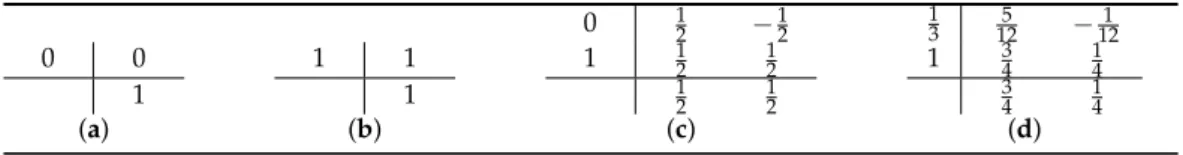
The noisy data is given byg^ε(s) =exp(sin(πs)/π²) +εcos(100s), s∈[0, 1], and the exact solution isw∗(t) =sin(πt). In order to demonstrate the results in Theorems1and 4, we consider Landweber, Levenberg–Marquardt (LM), Lobatto IIIC, and the Radau IIA methods, see Table1for the Butcher tableau.

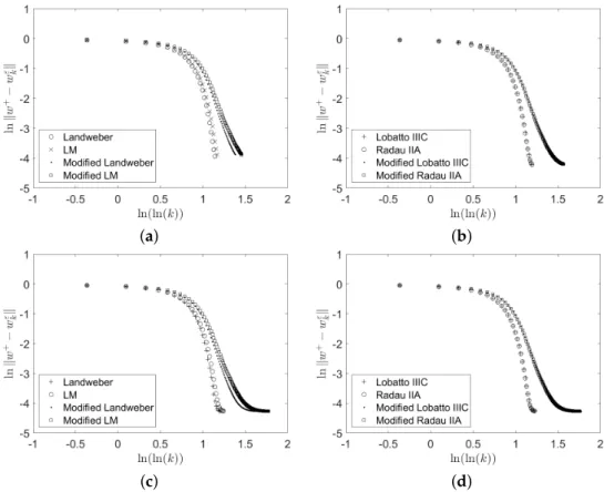
The implementation in this section is the same as the one reported in [10,13]. The num- ber of basis functions is 65 and the number of equidistant grid points is 150, while the parameterτ_kis the harmonic sequence term(_k+₁)^1.1. As expected, the results in Figure2 show that the curve of lnkw⁺−w^ε_kklies below a straight line with slope−p, as suggested by (30) in Theorem1and (70) in Theorem4.

Table 1. Butcher tableau for (a) explicit Euler or Landweber, (b) implicit Euler or Levenberg–

Marquardt, (c) Lobatto IIIC, and (d) Radau IIA methods.

0 ¹₂ −¹₂ ¹_{3 12}⁵ −₁₂¹

0 0 1 1 1 ¹₂ ¹₂ 1 ³₄ ¹₄

1 1 ¹₂ ¹₂ ³₄ ¹₄

(a) (b) (c) (d)

(a) (b)

(c) (d)

Figure 2. The plot of lnkw⁺−w_k^εk versus ln(_ln(k)) for (a) one−step RK methods and (b) for two−step methods withε=10⁻³. (c,d) Results withε=10⁻⁴. The parametersγare (a) 1.1, (b) 25, (c) 1.1, and (d) 100. For (a–d), a harmonic sequenceτ_k= (k+1)^1.1andw₀=εw∗are used.

6. Summary and Outlook

Up to now, the logarithmic convergence rate under logarithmic source condition has only been investigated for particular examples, namely, the Levenberg–Marquardt method (Böckmann et al. [21]) and the modified Landweber method (Pornsawad et al. [22]).

Here, we extended the results to the whole family of Runge–Kutta-type methods with and without modification. For the future, it is still open to prove the optimal convergence rate under Hölder source condition for the whole family without modification.

Author Contributions: The authors P.P., E.R., and C.B. carried out jointly this research work and drafted the manuscript together. All the authors validated the article and read the final version. All authors have read and agreed to the published version of the manuscript.

Funding:This research received no external funding.

Acknowledgments:The authors are grateful to the referees for the interesting comments and sug- gestions that helped to improve the quality of the manuscript.

Conflicts of Interest:The authors declare no conflict of interest.

References

1. Morozov, V.A. On the solution of functional equations by the method of regularization. Sov. Math. Dokl.1966,7, 414–417.

2. Tikhonov, A.N.; Arsenin, V.Y.Solutions of Ill Posed Problems; V. H. Winston and Sons: New York, NY, USA, 1977.

3. Bakushinsky, A.B.; Kokurin, M.Y. Iterative Methods for Approximate Solution of Inverse Problems; Springer: Berlin/Heidelberg, Germany, 2004.

4. Kaltenbacher, B.; Neubauer, A.; Scherzer, O.Iterative Regularization Methods For Nonlinear Ill-Posed Problems; Walter de Gruyter:

Berlin, Germany, 2008.

5. Hanke, M.; Neubauer, A.; Scherzer, O. A convergence analysis of the Landweber iteration for nonlinear ill-posed problems.

Numer. Math.1995,72, 21–37, doi:10.1007/s002110050.

6. Hochbruck, M.; Hönig, M. On the convergence of a regularizing Levenberg-Marquardt scheme for nonlinear ill-posed problems.

Numer. Math.2010,115, 71–79, doi:10.1007/s00211-009-0268-9.

7. Jin, Q. On a regularized Levenberg-Marquardt method for solving nonlinear inverse problems. Numer. Math.2010,115, 229–259, doi:10.1007/s00211-009-0275-x.

8. Hanke, M. The regularizing Levenberg-Marquardt scheme is of optimal order. J. Integral Equ. Appl.2010,22, 259–283.

9. Tautenhahn, U. On the asymptotical regularization of nonlinear ill-posed problems. Inverse Probl. 1994, 10, 1405–1418, doi:10.1088/0266-5611/10/6/014.

10. Böckmann, C.; Pornsawad, P. Iterative Runge-Kutta-type methods for nonlinear ill-posed problems.Inverse Probl.2008,24, 025002, doi:10.1088/0266-5611/24/2/025002.

11. Pornsawad, P.; Böckmann, C. Convergence rate analysis of the first-stage Runge-Kutta-type regularizations. Inverse Probl.2010, 26, 035005.

12. Scherzer, O. A modified Landweber iteration for solving parameter estimation problems. Appl. Math. Optim.1998,38, 45–68, doi:10.1007/s002459900081.

13. Pornsawad, P.; Böckmann, C. Modified iterative Runge-Kutta-type methods for nonlinear ill-posed problems. Numer. Funct.

Anal. Optim.2016,37, 1562–1589, doi:10.1080/01630563.2016.1219744.

14. Pornsawad, P.; Sapsakul, N.; Böckmann, C. A modified asymptotical regularization of nonlinear ill-posed problems. Mathematics 2019,7, 419, doi:10.3390/math7050419.

15. Zhang, Y.; Hofmann, B. On the second order asymptotical regularization of linear ill-posed inverse problems. Appl. Anal.

2018, 1–26, doi:10.1080/00036811.2018.1517412.

16. Hohage, T. Logarithmic convergence rates of the iteratively regularized Gauss-Newton method for an inverse potential and an inverse scattering problem. Inverse Probl.1997,13, 1279–1299.

17. Deuflhard, P.; Engl, W.; Scherzer, O. A convergence analysis of iterative methods for the solution of nonlinear ill-posed problems under affinely invariant conditions. Inverse Probl.1998,14, 1081–1106, doi:10.1088/0266-5611/14/5/002.

18. Hohage, T. Regularization of exponentially ill-posed problems. Numer. Funct. Anal. Optimiz.2000,21, 439–464.

19. Pereverzyev, S.S.; Pinnau, R.; Siedow, N. Regularized fixed-point iterations for nonlinear inverse problems. Inverse Probl.2005, 22, 1–22, doi:10.1088/0266-5611/22/1/001.

20. Mahale, P.; Nair, M.T. A simplified generalized Gauss-Newton method for nonlinear ill-posed problems. Math. Comput.2009, 78, 171–184.

21. Böckmann, C.; Kammanee, A.; Braunß, A. Logarithmic convergence rate of Levenberg–Marquardt method with application to an inverse potential problem.J. Inverse Ill-Posed Probl.2011,19, 345–367, doi:10.1515/jiip.2011.034.

22. Pornsawad, P.; Sungcharoen, P.; Böckmann, C. Convergence rate of the modified Landweber method for solving inverse potential problems. Mathematics2020,8, 608.

23. Vainikko, G.; Veterennikov, A.Y.Iteration Procedures in Ill-Posed Problems; Nauka: Moscow, Russia, 1986.