Disentangling and quantifying contributions of distinct forcing factors to the observed global sea level pressure field

(1)

https://doi.org/10.1007/s00382-019-05067-7

Disentangling and quantifying contributions of distinct forcing factors to the observed global sea level pressure field

Petru Vaideanu^1,2 · Mihai Dima^1,2 · Razvan Pirloaga³ · Monica Ionita²

Received: 20 June 2019 / Accepted: 27 November 2019

Abstract

Variations of the global sea level pressure (SLP) field reflect atmospheric and oceanic influences and have a profound influence on temperature, precipitation and the global carbon cycle. The impact of various forcing factors on this field was investigated mainly based on numerical simulations. Alternatively, here we identify and quantify the influences of various forcing factors on observational, reanalysis and simulated SLP fields. By applying canonical correlation analysis (CCA) on the aforementioned data sets, we separated and quantified the impact of increase CO₂ concentration, El Niño–Southern Oscillation (ENSO), Atlantic Multidecadal Oscillation (AMO), Arctic Oscillation (AO) and solar forcing on the global SLP field, based on their associations with known footprints on the sea surface temperature (SST). Together, their corresponding SLP spatial structures explain ~ 60% of the observed variance. Whereas the atmospheric CO₂ concentration has the most prominent impact on the global SLP field, explaining 28% of variance, ENSO and AO account for 9% each. The solar forcing and AMO explain 7%, respectively 6% of global SLP variance. Similar spatial structures corresponding to the same forcing factors are identified based on the reanalysis SLP data. CCA applied on simulated SLP fields derived from six CMIP5 model simulations captures only the spatial structures of atmospheric CO₂ concentration, ENSO, AAO and AO. Such a decomposition of the global pressure field based on a linear combination of coupled SST-SLP pairs provide a reference against which one could validate the performance of general circulation models in simulating the lower atmosphere dynamics.

Keywords Sea level pressure · Ocean temperature · CO₂ · Internal modes of variability · Solar influence

1 Introduction

One of the definitory property of the climate system is its significant complexity, resulting, for example, from the interactions between its components (e.g. atmosphere, ocean, land), which are characterized by very different characteristics. Consequently, the understanding of physical

mechanisms generating climate variability relies on simpli- fying assumptions about its dynamics. One of these hypoth- eses is that climate variations result from a combination of fluctuation induced by external causes and internal factors generated by interactions between components of the climate system. Whereas the former type of causes includes, for example, anthropogenic greenhouse gases, changes in solar irradiance, volcano eruptions, the internal fluctuations could be related to the El Niño–Southern Oscillation (ENSO) phenomenon, the Atlantic Multidecadal Oscillation (AMO) and other climate modes of variability. The identification of the footprints of such forcing factors (which could be of external or internal origin) on global fields and a quantification of their associated contributions to climate variations could significantly improve the understanding of atmosphere/ocean dynamics.

One key component to analyze the large-scale atmospheric circulation is sea level pressure (SLP). It encapsu- lates important information about atmospheric dynamics, but it is also under the influence of surface ocean conditions.

Electronic supplementary material The online version of this article (https ://doi.org/10.1007/s0038 2-019-05067 -7) contains supplementary material, which is available to authorized users.

* Petru Vaideanu

vaideanu.petru@yahoo.com

1 Faculty of Physics, University of Bucharest, Bucharest, Romania

2 Alfred Wegener Institute for Polar and Marine Research, Bremerhaven, Germany

3 National Institute of Research and Development for Optoelectronics, Măgurele, Romania

(2)

Furthermore, it reflects the atmospheric conditions at the Earth surface, in which the human activity is embedded.

Annular modes are the dominant structures of atmospheric variability in the extratropics, being associated with zonally symmetric negative (positive) pressure anomalies over the poles and positive (negative) ones at mid-latitudes (Thompson et al. 2000). Their representations in climate models are associated with some divergence, especially at high latitudes (Deser et al. 2012).

The Arctic Oscillation (AO; Lorenz 1951; Thompson and Wallace 1998) or the Northern Annular Mode (NAM) (Thompson et al. 2000) has a profound impact on temperature and precipitation in North America and Europe, as well as on sea ice distribution in the Arctic region (e.g.: Deser et al. 2000). The regional manifestations of AO in the North Pacific and in the North Atlantic boreal winter are known as the North Pacific Oscillation (Linkin and Nigam 2008) and the North Atlantic Oscillation (NAO) (Exner 1913; Hurrell 1995), respectively. Although there are differences between the spatial patterns of AO and NAO, it was proposed that these two modes are closely linked, so that they represent manifestations of the same mode of atmospheric variability (Hurrell and Deser 2009).

The dominant structure of the largescale atmospheric circulation of the Southern Hemisphere (SH), the Antarctic Oscillation (AAO) (Rogers and van Loon 1982; Gong and Wang 1999) or the Southern Annular Mode (SAM) (Thomp- son et al. 2000) defined in the geopotential height, is associated with the poleward contraction and strengthening of the SH westerly wind jet. It generates more rainfall and lower temperatures in the high latitudes and less rainfall and higher temperatures in the midlatitudes (Gillett et al. 2006; Mar- shall 2007). The physical mechanisms associated to SAM could be understood in terms of a positive feedback between the zonal wind and fluxes of transient eddy momentum (Lor- enz and Hartmann 2001).

In the tropical Pacific, the Southern Oscillation (SO) modulates the behavior of the atmosphere on interannual timescales and is characterized by a dipole of opposing sign pressure anomalies located in the eastern and in the western parts of this basin (Trenberth and Caron 2000). The SO could be linked to tropical ocean–atmosphere interactions associated with the El Niño–Southern Oscillation phenomenon (ENSO; Philander 1990; Deser et al. 2010).

The variability of the annular modes can be influenced by both, internal and external forcing factors. Previous studies based on observed and simulated data have linked changes in the evolution of the annular modes with the increase in greenhouse gases (GHG) emissions (Fyfe et al. 1999; Gillett and Thompson 2003; Gillett and Fyfe 2013), with the depletion of stratospheric polar ozone (Solomon 1999; Thomp- son et al. 2011; Gillett et al. 2013), with volcanic eruptions (Stenchikov et al. 2002; Christiansen 2008; McGraw

et al. 2016), with changes in solar irradiation (Kuroda and Kodera 2005; Huth et al. 2007; Roscoe and Haigh 2007;

Hood et al. 2013) or with natural variability (Ruprich-Robert et al. 2017). It was proposed that changes in solar irradiance and in mean temperature over the Northern Hemisphere played an important role in modulating the SO over the last 2000 years (Yan et al. 2011). However, there is no consensus about the relative contributions of these forcing factors to the annular modes in a changing climate (IPCC 2013).

The evolution of the SLP field has long been linked with changes in sea surface temperature (SST) over both the Pacific and the Atlantic basins (e.g.: Bjerknes 1969; Zorita et al. 1992). The goal of this study is to identify and quantify the contributions of main forcing factors to the global SLP field. Section 2 includes a presentation of the data and of the statistical methods used in this study. In Sect. 3, we analyze the coupled global SST-SLP patters and attribute them to forcing factors. The conclusions are formulated in Sect. 4.

2 Data and methods

2.1 Data

Observational SLP and SST fields used here were downloaded from the Met Office Hadley Centre’s (HadSLP2—

Allan and Ansell 2006; HadISST—Rayner et al. 2003).

The HadSLP2 data (5° × 5° grid) was developed using marine observations from International Comprehensive Ocean–Atmosphere Data Set (ICOADS) and land observations from 2228 stations all over the globe (Allan and Ansell 2006). The HadISST (1° × 1°) fields are reconstructed using a two-stage reduced-space optimal interpolation procedure, followed by superposition of quality improved grid- ded observations onto the reconstructions, to restore local detail. For comparison, we used the version 5 of the ERSST (2° × 2°) data set (Huang et al. 2017).

The instrumental AAO Index, the AO Index, the Niňo3 Index, the AMO Index, the SO Index, the 10.7 cm Solar Flux Index and the CO₂ concentration recorded at Mauna Lua Observatory are obtained from the National Oceanic and Atmospheric Administration (http://www.esrl.noaa.gov/

psd/data/clima teind ices/list/). Please see Table S1 for more information about the climate indexes used here.

We used also the NCEP/NCAR Reanalysis SLP and SAT data from the National Centre for Atmospheric Research (NCAR) and the National Centre for Environmental Pre- diction (NCEP), (Kalnay et al. 1996). The NCEP/NCAR Reanalysis project is using a state-of-the-art analysis/fore- cast system to perform data assimilation using past data from 1948 to the present. Assimilation of surface, satellite, radiosonde and other observations of pressure, temperature,

(3)

humidity and other variables are used to create fields distributed on a 2.5° × 2.5° grid.

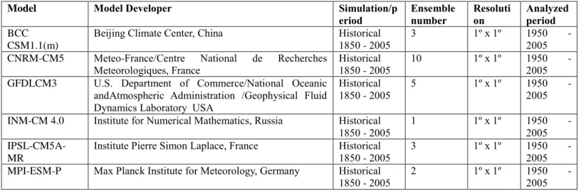
Modeled SST and SLP data used here are from “His- torical” CMIP5 simulations, distributed on a 1° × 1° grid.

The simulations extend over the 1850–2005 period and are performed with observed forcing agents like anthropogenic CO₂ emissions, volcanic aerosols and solar forcing (Taylor et al. 2012). We used a mean of six CMIP5 models (BCC_CSM1.1 (m), CNRM-CM5, GFDLCM3, INM- CM4.0, IPSL-CM5A-MR, MPI-ESM-P) which were used in previous studies to investigate internal variability (Gillett and Fyfe 2013; Ham and Kug 2014; Han et al. 2016). Output data is downloaded from https ://clime xp.knmi.nl/selec tfiel d_cmip5 .cgi. For more information about the CMIP5 models used in this study are included in Table S2.

The analyses are performed based on annual values of SST and SLP. If monthly values are used, the results are qualitatively the same. Anomalies from the annual cycle were calculated for all datasets, as a preliminary operation.

2.2 Methods

We used the Empirical Orthogonal Functions (EOF) method (Lorenz 1956) to identify the dominant modes of global atmospheric variability. The EOF analysis is used to identify spatial patterns of variability (EOF’s) in association with a principal component (PC) time series. It can be used to identify dominant patterns and to increase the signal-to-noise ratio in the analyzed field.

Coupled patterns are identified here through Canonical Correlation Analysis (CCA; von Storch and Zwiers 1999), in a similar manner as in Zorita et al. (1992). CCA is a multivariate statistical technique which is applied to two data sets in order to identify pairs of spatial structures associated with maximum correlated temporal evolutions. The main criteria for ranking the resulting pairs is the correlation coefficient between the pairs of patterns (vectors), unlike similar statistical methods which maximize the variance/covariance.

The CCA procedure includes several steps: (i) a prefiltering of the two initial fields by decomposing the initial fields through EOF analysis and the reconstructing it back based on a reduced number of modes, (ii) normalizationthe PCs and construction of a covariance matrix based only on a subset of them, which accounts for most of the variance;

(iii) identification of the correlation coefficients by applying the Singular Value Decomposition (SVD) method to the covariance matrix of the PCs. In our study we used CCA to identify coupled SST-SLP modes and their associated time components. The combined explained variance of the selected EOFs is over 70% for HadSLP2/HadISST (the first 10 EOFs), NCEP/NCAR data (the first 14 EOFs) and CMIP5 data (the first 6 EOFs).

The statistical significance of correlations is estimated through a two-tailed t test. The number of degrees of freedom is computed based on the lag-1 autocorrelation of the two-time series (Bretherton et al. 1999).

Observed, reanalysis and CMIP5 SLP and SST data are used in a complementary way. The effects of imperfections and possible biases in the observational data are reduced by using multivariate statistical methods which are effi- cient in increasing the signal-to-noise ratio. Except for removing the annual cycle, no pre-filter of the data was performed before EOF analyzes.

The decrease in signal in SLP and SST observations prior to 1950 has been well documented (Deser et al.

2010). In order to better compare the results derived from observations with the ones from numerical simulation, we performed the CCA’s for the 1950–2005 period using the HadSLP2 and CMIP5 SLP data. Over this time interval (1950–2005) the atmospheric CO₂ concentration shows a prominent growing trend, whereas the solar forcing is marked by a slight decreasing trend. These different evolutions are increasing the chances to separate the impact of anthropogenic from that of the solar forcing. Similar results are also obtained if ErSSTv5 data are used (not shown).

2.3 Strategy

The EOF method separates orthogonal spatial patterns in a given field. As each mode could be excited by several different forcing factors, although such decomposition could significantly reduce the number of degrees of freedom, it does not necessarily isolate the footprint of a specific forcing on climate.

The CCA is applied to two fields in order to identified pairs of patterns whose associated time series are maximum correlated. Therefore, whereas EOF is based on the distinction between patterns (they are orthogonal), CCA is based on the distinction between time evolutions of spatial structures (time series of consecutive pairs are uncorrelated). If one assumes that distinct forcing factors are characterized by different temporal evolutions, which is a reasonable hypoth- esis for sufficiently long time intervals, then CCA appears as a method which could be used to separate the footprint of forcing factors on a given field. Here we apply this method on SST and SLP data in order to identify the footprints of various potential causes of large-scale climate variability on this last global field. The attribution to a specific forcing of a SLP pattern provided by CCA (as part of a coupled SST-SLP pair), is established based on two criteria:

1. the corresponding SST pattern should be similar with that of the assumed forcing factor.

(4)

2. The temporal shape of the associated time series should be significantly correlated with that of the assumed forcing factor.

3 Results

3.1 Dominant global atmospheric modes

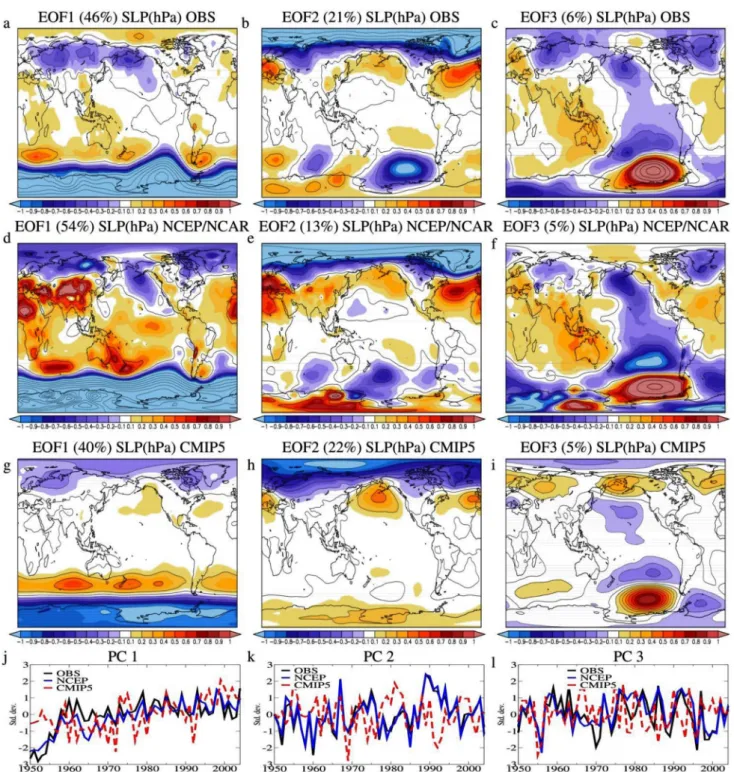
The first tree modes of global sea level pressure variability, derived through EOF analysis of the observed annual SLP anomalies over the 1950–2005 period, NCEP/NCAR reanalysis and CMIP5 data, are shown in Fig. 1. The cumulated explained variance of these tree modes is over 70% in observation/reanalysis data and 67% in CMIP5 fields.

The spatial structures of the dominant mode (EOF1) identified in observations (Fig. 1a), NCEP/NCAR (Fig. 1d) and CMIP5 (Fig. 1g) include the largest values in the SH.

The spatial structure of the EOF1 derived from observations (Fig. 1a) is dominated by negative pressure anomalies located over Antarctica, surrounded by positive pressure anomalies at mid-latitudes, which are characteristic for a positive AAO phase (Gong and Wang 1999). These features can be easily identified in the EOF1 patterns obtained using the reanalysis (Fig. 1d) and CMIP5 (Fig. 1g) data.

Minor differences between the three spatial structures can be identified around the North Pole. The EOF1 pattern from the reanalysis (Fig. 1d) is qualitatively similar with the observed (Fig. 1a) and simulated (Fig. 1g) EOF1 patterns, but the loadings are slightly overestimated, especially over the continents, in mid-latitudes. The spatial structure of the EOF1 derived from CMIP5 data (Fig. 1g) has the maxium meridional SLP gradient located slightly southward and a more zonally distributed pattern in the SH compared to both, observations and reanalysis. In the NH it resembles more the pattern from the reanalysis (Fig. 1d). An AAO signal has been previously identified in the CMIP5 data, although there are some differences between models for the spatial pattern (e.g.: Raphael and Holland 2006). The associated PC’s of the dominant modes (Fig. 1j) are strongly correlated with AAO Index (Table 1) and show a slightly increasing trend, in good agreement with previous studies (Marshall 2003), further indicating that this mode reflects mainly AAO variations.

The spatial structures of the second EOF derived from observed, reanalysis and CMIP5 SLP data is shown Fig. 1b, e and h respectively. In the NH, the three spatial structures are qualitatively similar and resemble a positive phase of the AO, with negative anomalies at high latitudes and two centers of positive anomalies in the North Atlantic and North Pacific basin (Thompson et al. 2000). Compared to observations, there is a small tendency to overestimate SLP anomalies in the NCEP/NCAR data (Fig. 1e) and a more prominent center of positive anomalies in the North Pacific

basin for the CMIP5 data. The PC’s of the observed and NCEP/NCAR EOF1 are strongly correlated between them and with the AO Index (Table 1) and show an increasing trend over the 1965–1995 period, which is not captured in the CMIP5 PC (Fig. 1k). In synthesis, this mode reflects mainly AO variations.

The two spatial structures of the third EOF identified in observations (Fig. 1c) and in the NCEP/NCAR fields (Fig. 1f) are qualitatively similar and include a zonal seesaw of SLP anomalies in the Tropical Pacific basin, between Darwin and Tahiti and successions of centers of alternating signs emerging from western tropical Pacific and extending poleward and eastward in both hemispheres, resembling Rossby waves propagations. These atmospheric features are consistent with a tropical forcing and are associated with the SO (Trenberth and Caron, 2000) and are less prominent in CMIP5 EOF3 (Fig. 1i). This association is also supported by the correlation between the PC’s of this mode and the SO Index (Table 1).

Although both the AAO and the AO are active all year around, their impact is more pronounced in the cold season.

To further investigate the association of EOF1 and EOF2 with AAO and AO, we compared the global structures with the ones derived from regional seasonal EOF analyses (Supp. Figure 2). In the SH, for June–July–August (JJA), we found a dominant structure (EOF1, Supp. Figure 2c, d) which is similar with the one described in association with AAO (Fig. 1a, d). Also, the correlation coefficients between the PC’s of the EOF1 derived from the global SLP field and the PC of the EOF1 derived from NH JJA anomalies are close to 0.9 (statistically significant at > 99% confidence level) for HadSLP2 and NCEP/NCAR data. In the NH, for December–January–February (DJF), the dominant spatial structure (EOF1) is similar with the global structure, derived from observed and NCEP/NCAR data, associated to AO (Fig. 1b, e). The correlation coefficients between the associated time series from EOF1 NH DJF (Supp. Figure 2g, h) and from EOF2 global (Fig. 1k) are strongly correlated (r > 0.85, > 99% confidence level).

In summary, the three dominant global modes are qualitatively similar in observations, reanalysis and simulated data. A tendency to overestimate SLP anomalies is noted in the NCEP/NCAR data, especially over the continents.

The association of the global EOF patterns to known atmospheric annular modes is supported by the strong correlation between the PC’s and the corresponding indexes (Table 1) and by the similarities with the results obtained from regional/seasonal EOF analyses (Supp. Figure 2).

3.2 Observed coupled global SST‑SLP pairs

In order to identify global coupled SST-SLP pairs, CCA was performed between the corresponding annual fields from the

(5)

Fig. 1 Observed, reanalysis and simulated global modes of sea level pressure variability. Top row: The leading empirical orthogonal function (EOF) of the global sea level pressure anomalies (hPa) extending over the 1950–2005 period, based on HadSLP2 (a), NCEP/NCAR (b) and CMIP5 (c) data sets. Second row: The second empirical orthogonal function (EOF) of the global sea level pressure anomalies (hPa) extending over the 1950–2005 period, based on HadSLP2 (d), NCEP/

NCAR (e) and CMIP5 (f) data sets. Third row: The third EOF of the global sea level pressure anomalies (hPa) extending over the 1950–

2005 period, based on HadSLP2 (g), NCEP/NCAR (h), CMIP5 (i) data sets. Bottom row: the time components associated to the EOF1 (j), EOF2 (k) and EOF3 (l) derived from HadSLP2 (black line), 20CR (blue line) and CMIP5 (red line) data sets

(6)

HadISST and HadSLP2 datasets, for the 1950–2005 period, with the results shown in Fig. 2 and Table 2.

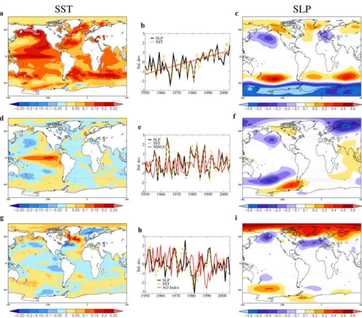
The SST spatial structure of the first SST-SLP pair (Fig. 2a) is dominated by positive anomalies extending all over the globe, suggesting an association with the greenhouse effect induced by the atmospheric CO₂, which is also supported by the corresponding increasing trend which dominates its time component (Fig. 2b). The global SLP spatial structure (Fig. 2c,) is dominated by negative anomalies over the polar regions, extending also over North Pacific and Eurasia and by a zonal band of positive values located between 50° S and 50° N. A similar structure was associated with human influence (mostly emissions of greenhouse gases (GHGs) and tropospheric sulphate aerosols) in a previous numerical study (Gillett et al. 2003). In the North Atlan- tic, a pattern similar to the positive NAO phase is observed, which was simulated in response to increased anthropogenic greenhouse gases (Kuzmina et al. 2005; Stephenson et al.

2006). In the Southern Hemisphere, a prominent positive AAO-like structure appears in both the observed and reanalysis spatial structures, which also was simulated in response to increasing GHGs (Fyfe et al. 1999; Arblaster and Meehl 2006). CMIP5 models also project with high confidence a trend in the AAO over the 21st century, as a result of increasing GHGs (Gillett and Fyfe 2013). The centers of negative SST anomalies located south-east from Greenland and in North Pacific appear to be generated by southeast- ward cold air advection, in association with the relatively strong wind inferred from the corresponding SLP pattern (Fig. 2c). The SST anomalies around Antarctica appear also to be induced by the anomalous winds related to the maximum SLP gradient in this area. These features provide mutual physical consistency to this coupled SST-SLP pair.

The quasi-uniform positive SST anomalies dominating the global structure (Fig. 2a, d), the structure of the SLP pattern (Fig. 2c, f) in combination with previous observational and numerical studies, but also the trend of the corresponding time components (Fig. 2b), indicate in a convergent way that

this pair is associated with the atmospheric CO₂ increase.

The atmospheric structure of this pair explains 28% of variance in the global SLP field and projects (Table 2) on EOF1 (Fig. 1a) and EOF2 (Fig. 1b).

The SST spatial structure of the second pair (Fig. 2d) is dominated by pronounced SST anomalies in the tropical Pacific, with a band of warm SST starting from the west coast of Peru, surrounded by negative loadings off the coast of Australia, New Zealand and Japan. This SST spatial pattern has the characteristics of the ENSO phenomenon, the main source of interannual variability in the climate system (e.g.: Philander 1990; Deser et al. 2010). The temporal evolution of the SST/SLP structures (Fig. 2e) are dominated by interannual variability and are significantly correlated with the Niño3 index (r = 0.74, > 95% significance level), further supporting the association of this pair with ENSO. The SLP spatial structure (Fig. 2f) includes a dipole in the tropical Pacific, with low SLP in the Eastern Pacific and positive values in the Western sector of this basin. In the high latitudes, in the SH we find a strong projection of ENSO onto Amundsen Sea low (ASL; Turner et al. 2013) and in the NH onto AO, through Rossby waves excited by deep convection associated to El-Niño events (e.g.: Trenberth et al. 1998;

Ciasto et al. 2015). The SLP pattern from this pair reflects ENSO variations, it explain 9% of variance in the global field and it projects strongly (Table 2) on EOF3 (Fig. 1c).

The SST pattern of the third pair (Fig. 2g) has the maximum anomalies over the subpolar gyre and is characterized by uniform positive anomalies in North Atlantic, loadings of opposite sign in the South Atlantic and negative anomalies in the Eastern Tropical Pacific. These features are repre- sentative for the Atlantic Multidecadal Oscillation (AMO;

Kerr 2000). The AMO is linked to fluctuations in the Atlan- tic Meridional Overturning Circulation (AMOC; Latif et al.

2004; Knight et al. 2005; Gulev et al. 2013; Ionita et al.

2016) and has a global influence on climate (Sutton and Hodson 2005; Dima and Lohmann 2007; Ruprich-Robert et al. 2017; Vaideanu et al. 2018). The time series associated

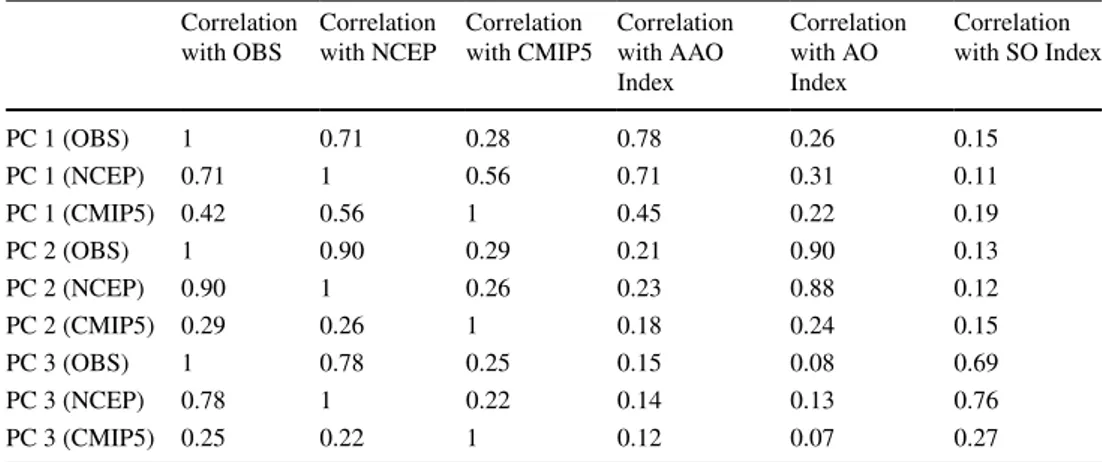
Table 1 Correlation coefficients (r) between the PCs of the EOFs derived from OBS, NCEP and CMIP SLP, over the 1950–2005 period, and AAO, AO and SO Index

Correlation

with OBS Correlation

with NCEP Correlation

with CMIP5 Correlation with AAO Index

Correlation with AO Index

Correlation with SO Index

PC 1 (OBS) 1 0.71 0.28 0.78 0.26 0.15

PC 1 (NCEP) 0.71 1 0.56 0.71 0.31 0.11

PC 1 (CMIP5) 0.42 0.56 1 0.45 0.22 0.19

PC 2 (OBS) 1 0.90 0.29 0.21 0.90 0.13

PC 2 (NCEP) 0.90 1 0.26 0.23 0.88 0.12

PC 2 (CMIP5) 0.29 0.26 1 0.18 0.24 0.15

PC 3 (OBS) 1 0.78 0.25 0.15 0.08 0.69

PC 3 (NCEP) 0.78 1 0.22 0.14 0.13 0.76

PC 3 (CMIP5) 0.25 0.22 1 0.12 0.07 0.27

(7)

to the coupled patterns (Fig. 2h) are significantly correlated with the AMO index (r = 0.63, > 95% significance level). The associated SLP spatial structure (Fig. 2i) includes negative anomalies over the North Atlantic, Europe and North Africa, and positive loadings over the poles and in the North Pacific.

The negative AO-like structure identified in the North Atlantic has been previously linked with the positive AMO phase (Dima et al. 2001; Omrani et al. 2014; Gastineau and Frankignoul 2015), with the atmosphere reflecting a local thermal influence from the ocean below. In the North Pacific, the weakening of the Aleutian low (Fig. 2i) appears to generate the positive SST anomalies off the cost of Japan through weak westerlies, reduced cold atmospheric advection and weak mixing in the ocean surface layers, consistent with previous studies witch show that the AMO has a strong influence on Pacific decadal variability (Dima and Lohmann 2007; Zhang and Delworth 2007; Zanchettin et al.

2016). In the high latitudes of the SH a AAO-like structure is observed, which is in good agreement with previous studies using numerical simulations investigating the impact of the AMO over this region (Li et al. 2014; Ruprich-Robert et al.

2017). The predominantly cold SST anomalies do not appear to be induced by the atmospheric circulation above them.

The time series (Fig. 3h), significantly correlated with the AMO index, together with the SST structure (Fig. 3g), characteristic for AMO, indicate that this coupled pair reflects the AMO footprint on these two fields. The associated SLP structure explains 6% of variance in the global SLP field and projects (Table 2) on EOF1 (Fig. 1a) and EOF 2 (Fig. 1b).

The SST field from the fourth pair (Fig. 2k) is characterized by a tripole of maximum SST anomalies in the North Atlantic, with positive values in the subpolar gyre, negative loadings in the western sub-tropical North Atlantic and warm anomalies between the equator and 30° N. This oceanic response is generated by the AO mainly through changes in the turbulent energy flux (Cayan 1992; Dima et al. 2001; Marshall et al. 2001; Deser et al. 2010). A similar atmosphere–ocean relation is observed in North Pacific region, but not around Antarctica. The corresponding time components (Fig. 2l) are significantly negatively correlated with AO Index. (r = − 0.67, > 95% significance level). The associated SLP spatial structure (Fig. 2m) has the most intense values in the NH, with positive loadings over the North Pole and negative anomalies in the North Atlantic and North Pacific basins, similar to the negative phase of AO.

This SLP structure explains 9% in the global SLP field and projects strongly (Table 2) on EOF2 (Fig. 1b).

The SST structure of the fifth pair derived through CCA (Fig. 2n) includes tilted bands of alternating sign in the Pacific basin, starting with negative anomalies West of South America and ending with a band of positive values westward from North America. In North Atlantic it includes a center of negative values. These were associated with solar forcing

in previous studies (White et al. 1997; Lohmann et al. 2004;

Dima et al. 2005; Meehl et al. 2008; Hood et al. 2013; Gray et al. 2013; Dima and Voiculescu 2016). The corresponding time components (Fig. 2o) are significantly correlated with the solar irradiance (r = 0.43 for the SLP time series, statistically significant at 90% confidence level), with a 4 years’

lag, consistent with a causal relationship between this natural forcing and the North Atlantic response (van Loon and Meehl 2014). The SLP spatial structure (Fig. 2p) includes the North Pacific Oscillation (NPO) pattern, which was also linked to solar variability (Roy and Haigh 2010; Hood et al.

2013; van Loon and Meehl 2014; Dima and Voiculescu 2016). These Pacific SST and SLP configurations indicate an atmospheric influence on the ocean surface thermal conditions in the Northern Hemisphere. The SLP center of negative anomalies located in the north-east Asia was also associated with the solar forcing (Hood et al. 2013). In the North Atlantic, a negative NAO-like structure is observed.

In the SH, the SLP pattern projects strongly on AAO. This response was linked to the solar forcing using proxy records (Abram et al. 2014), observational data (Kuroda and Kodera, 2005; Kuroda 2018) and simulations with climate models (Hood et al. 2013; Gillett and Fyfe 2013). The SLP pattern of this pair explains 6% in the global field and projects (Table 2) on EOF1 (Fig. 1a).

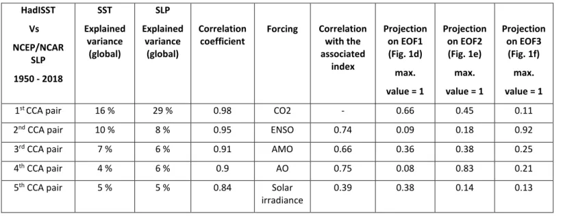
In order to test the robustness of the results on a different SLP dataset and time frame, we performed another CCA using the NCEP/NCAR Reanalysis SLP data, over the 1950–2018 period (Supp. Figure 4). All the pairs derived from reanalysis data are similar with the ones obtained from observation (Fig. 2). The NCEP/NCAR reanalysis appear to capture slightly better the coupled SST/SLP patterns associated with AO, but separates less precisely the AMO and the 11-year solar influence. The footprints of anthropogenic climate change and ENSO are quasi-identical to observations. The close similarity between the SST/SLP structures derived in observations and reanalysis indicates that these results are relevant for the global SLP variability.

In order to test the association to specific forcing factors of the SST-SLP pairs identified through CCA, we regressed the surface air temperature (SAT) field on the time components associated to the SST-SLP pairs from Fig. 2. The regression maps of SAT on the time series of the PC from the CCA pairs associated to ENSO (Supp.

Figure 3a) and NAO- (Supp. Figure 3c) are in very good agreement with previous studies (McPhaden et al. 2006;

Deser et al. 2010). The regression map of SAT on the PC of the SST-SLP pair associated to AMO (Supp. Fig- ure 3b) includes positive temperature anomalies over North America and most of the Arctic, which have been previously linked with the positive AMO phase (Ruprich- Robert et al. 2017). The regression map of SAT obtained using the PC from the CCA pair linked to solar influence

(8)

(9)

is characterized by positive values over the poles, more pronounced in the NH. An increase in SAT over the poles and a preference to warm the continents vs. the oceans as a result of solar influence has also been previously reported (Camp and Tung 2007; Tung and Camp 2008). They also find the solar link with these areas to be statistically significant, further supporting the association of the 5th pair derived from CCA to solar forcing.

The observed projections of the dominant EOFs on the SLP patterns derived through CCA (Table 2), indicate that the footprint of the increase in atmospheric CO₂ concentration and of the AMO on the global SLP field (Fig. 2c) results largely from a combination of EOF1 (AAO) and EOF2 (AO). Unlike this, the ENSO contribution to the global SLP variability (Fig. 2f) and the SLP global structure from the 4th pair (Fig. 2m) are generated almost entirely by EOF3 (SO) respectively by EOF2 (AO). The solar impact on the global SLP field is generated mainly through EOF1 (AAO). One notes that AAO appears to be linked to the atmospheric CO₂ concentrations, to AMO and to the solar irradiance variations, all these forcing factors projecting on the structure of this mode (Fig. 2c, i, p). Similar results regarding such projections are obtained using NCEP/NCAR SLP data (Supp. Table 3).

In summary, through a CCA applied on observational annual data, we identify coupled SST-SLP pairs of spatial structures which were attributed to distinct forcing factors, based on their spatial and temporal properties. Together, the five global SST/SLP spatial patterns explain more than 51%/59% (Table 2) of variance in these fields. The identification of all five footprints in the same analysis provides quantitative estimations of the contributions of important forcing factors to the variability of the global SLP field.

3.3 CMIP5 coupled global SST‑SLP pairs

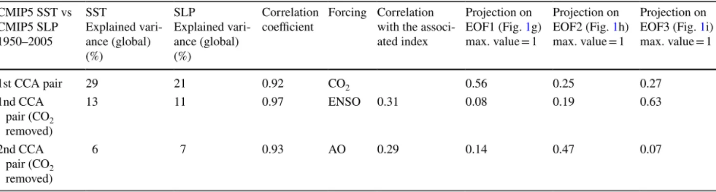
In order to investigate (by comparing with observations) the ability of the CMIP5 models to simulate the observed coupled SST-SLP pair, CCA’s were performed also on SST and SLP data from a mean of six CMIP5 models “Histori- cal” simulations (Table S2), over the same (1950–2005) period.

The SST spatial structure (Fig. 3a) of the most coupled SST-SLP pair captures the response of the ocean temperature to an increase in CO₂ concentrations (IPCC 2013) and is similar with the SST response from observations (Fig. 2a).

The temporal evolution of the two structures (Fig. 3b) is marked by an increasing trend. The associated SLP structure (Fig. 3c) shows a strong positive AAO response in the SH similar with previous investigations (Gillett and Fyfe 2013) and with observations (Fig. 2c). In the NH the response includes negative anomalies over most of Europe, North Africa and North Pacific, which is in contrast with both observations (Fig. 2c) and previous projections which show a weak but positive AO like response (Fyfe et al. 1999).

However, other studies, find trends of both signs (Gillett et al. 2003; Morgenstern et al. 2010) or even a negative shift in AO in response to GHG’s, mostly due to changes in Arctic sea ice (Jaiser et al. 2012; Cattiaux and Cassou 2013). The SLP pattern of this pair explains 21% in the global field and projects (Table 3) on EOF1 from CMIP5 data (Fig. 1g).

Because the simulated response to increased atmospheric CO₂ concentrations dominates the CMIP5 SST data (Supp.

Figure 5) due to the finite number of physical processes con- sidered in the numerical simulations and to the model imperfections, in order to facilitate the identification of the climate modes which have spatially heterogeneous patterns, before a second CCA, the trend was removed from the simulated SST data by subtracting from each grid point the annual global average. Similar results are obtained if we remove EOF1 from both the SST and SLP data (not shown). The first coupled simulated SST-SLP pair, obtained through this second CCA, after the trend was removed, is shown in Fig. 3d–f.

The SST pattern (Fig. 3d) is dominated by a band of positive anomalies in the Eastern tropical Pacific and is similar with the observed SST pattern associated to ENSO (Fig. 3d), except the Indian Ocean. However, the correlation between the associated time series and the Niño3 Index is much lower than in observations (r = 0.31 vs r = 0.76) in good agreement with previous studies indicating that consensus in the CMIP5 models regarding how ENSO will respond to 21^st century climate change has not been reached (Achuta- Rao and Sperber 2006; Collins et al. 2011; Stevenson et al.

2012). The associated SLP structure has a zonal seesaw of SLP anomalies in the tropical Pacific and a weakening of the ASL in the SH, similar with the observed pattern reflecting the ENSO phenomenon (Fig. 2d). This SLP pattern explains

Fig. 2 Coupled SST-SLP pairs derived through CCA between the corresponding HadISST and HadSLP2 fields over the 1950-2005 period. Top row: The 1st most coupled CCA pair: The SST pattern (a) explaining 21% of variance and the SLP structure (c), explaining 28% of variance. Their temporal evolution (b) has a correlation coefficient of 0.98. Second row: The 2nd most coupled CCA pair: The SST pattern (d) explaining 11% of variance and the SLP structure (f), explaining 9% of variance. Their temporal evolution (e) has a correlation coefficient of 0.97. Their correlation with the Niño3 index (e, red line) is 0.76. Third row: The 3rd most coupled CCA pair: The SST pattern (g) explaining 8% of variance and the SLP structure (i), explaining 5% of variance. Their temporal evolution (h) has a correlation coefficient of 0.93. Their correlation with the AMO index (h, red line) is 0.63. Fourth row: The 4th most coupled CCA pair: The SST pattern (k) explaining 5% of variance and the SLP structure (m), explaining 9% of variance. Their temporal evolution (l) has a correlation coefficient of 0.9. Their correlation with the negative AO index (l, red line) is 0.68. Fifth row: The 5th most coupled CCA pair: The SST pattern (n) explaining 6% of variance and the SLP structure (p), explaining 8% of variance. Their temporal evolution (o) has a correlation coefficient of 0.88. Their correlation with the 10 cm Solar Flux Index (o, red line, plotted with a 4 year lag) is 0.43 (with lag 4)

◂

(10)

11% of variance in the global field and projects (Table 3) on EOF3 from CMIP5 data (Fig. 1i).

The SST spatial structure of the second simulated pair obtained through CCA, after the trend was removed (Fig. 3g), includes a tripole of SST anomalies in the North Atlantic, similar with the response of the SST to AO identified in observations (Fig. 2k). The temporal evolution (Fig. 3h) has a much lower correlation with AO Index (r < − 0.3), compared to observations. It has been argued that future projections regarding the evolution of AO are depend- ent on the way models simulate troposphere-stratosphere interactions (Sigmond and Scinocca 2010; Karpechko and Manzini 2012). The associated SLP structure, has the most intense values in the NH and is similar with the observed global SLP pattern associated with AO (Fig. 2m) and with previous studies investigating the representation of AO pattern in CMIP models (Miller et al. 2006). This SLP structure explains 7% in the global SLP field and projects (Table 3) on EOF2 from CMIP5 data (Fig. 1h).

Although an AMO-like structure has been identified in the SST data (Supp. Figure 5c) we were not able to associate a SST-SLP pair to this climate mode trough CCA, indicating that the CMIP5 models analyzed here do not simulate the atmospheric teleconnections related to this climate mode.

This is not totally unexpected, since not much progress has been made between CMIP3 and CMIP5 simulations regarding the AMO (Ruiz-Barradas et al. 2013). Solar influence on SST-SLP (Fig. 2n–p) was also not detected trough CCA on CMIP5 SST and SLP data.

Compared to observations, the six CMIP5 models used here simulate well the spatial patterns of the coupled SST- SLP pairs associated to increased GHG’s, ENSO and AO.

However, they do not reproduce the temporal evolution of the associated indexes (Table 3) making difficult the inter- pretation of the 21st century projections regarding these climate phenomena.

To summarize the results, trough EOF analysis we identified the dominant modes of SLP variability in observed, reanalysis and CMIP5 SLP data. Through CCAs we separate

the contributions of five forcing factors to the global SST/

SLP fields. Furthermore, by projecting the dominant EOFs on the SLP structures identified through CCA we estimate the contributions of the dominant eigenmodes to the footprint of each forcing factor on the SLP field.

4 Discussion and conclusions

Trough EOF analysis on observed, reanalysis and CMIP5 SLP data, we have shown that 60% the global SLP variability over the 1950–2005 period is explained by the dominant three modes of atmospheric variability. This implies that the mechanisms through which different forcing factors affect the lower atmosphere dynamics are likely to be related to the physics of these three modes.

The first EOF on all three SLP data sets shows that since 1950, the AAO presents an increasing trend. As numerical simulations show, an increase in the greenhouse gas concentration is reflected in a warming of the troposphere and a cooling of the stratosphere and results in an increase of the meridional temperature gradient in the atmosphere. This drives an acceleration and a poleward shift of the SH tropospheric jet, resulting in the positive AAO trend (Fyfe et al.

1999; Arblaster and Meehl 2006; Miller et al. 2006; Gillett et al. 2013). However, the amplitude of the increase is different from observations (Gillett et al. 2003). Fluctuations in the solar forcing changes also the latitudinal gradient of radiative heating in the upper stratosphere, due to changes in UV absorption and ozone production and could have an impact on SAM (Kodera and Kuroda 2002; Kuroda 2018).

Trough propagation of Rossby waves, the tropical and North Atlantic also have an impact on the SH atmospheric circulation changes (Li et al. 2014).

Over the last part of the 20th century, as shown in the second EOF (Fig. 1), AO has an increasing trend (Hurrell and Deser 2009) which was linked to human influence (Fyfe et al. 1999; Gillett et al. 2003). However, more recent studies show that increase in GHG’s can also lead to a negative

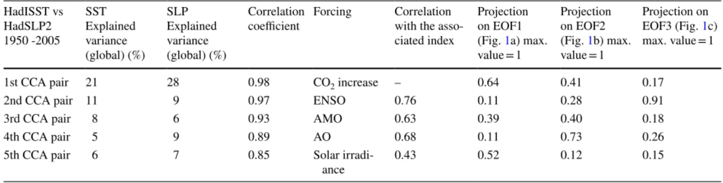
Table 2 The variances explained by each pattern and the correlation coefficients between the CCA’s time series from Fig. 2 extending over the 1950–2005 period

HadISST vs HadSLP2 1950 -2005

SSTExplained variance (global) (%)

SLPExplained variance (global) (%)

Correlation

coefficient Forcing Correlation with the associated index

Projection on EOF1 (Fig. 1a) max.

value = 1

Projection on EOF2 (Fig. 1b) max.

value = 1

Projection on EOF3 (Fig. 1c) max. value = 1

1st CCA pair 21 28 0.98 CO₂ increase – 0.64 0.41 0.17

2nd CCA pair 11 9 0.97 ENSO 0.76 0.11 0.28 0.91

3rd CCA pair 8 6 0.93 AMO 0.63 0.39 0.40 0.18

4th CCA pair 5 9 0.89 AO 0.68 0.11 0.73 0.26

5th CCA pair 6 7 0.85 Solar irradi-

ance 0.43 0.52 0.12 0.15

(11)

phase of AO through sea ice loss (Jaiser et al. 2012; Catti- aux and Cassou 2013). Solar influence on the North Atlan- tic is not asymmetric relative to the phase of the forcing and that the structure of the response in this sector changes over a solar cycle (Ineson et al. 2011; van Loon and Meehl 2014). The AO is affected also by the Eurasian snow cover (Cohen and Jones 2011), Arctic sea ice (Li and Wang 2013) or ENSO (Mathieu et al. 2004).

Through a single CCA analysis based on observations, we quantified the contributions of five forcing factors to

the global SLP variability: atmospheric CO₂ concentration (28%), ENSO (9%), AO (7%), AMO (6%) and changes in total solar irradiance (7%). Furthermore, we estimate how much contributes each of the dominant three EOFs to the impact of each forcing factor on the global SLP field. The SLP spatial structures associated to changes in CO₂ concentration and AMO result from a combination of EOF1 (AAO) and EOF2 (AO), the footprint of ENSO is generated mainly by EOF3 (SO), the SLP global structure associated to Atlantic tripole results almost entirely from EOF2 (AO)

Fig. 3 Coupled pairs derived through CCA between the corresponding CMIP5 SST/SLP fields over the 1950–2005 period. Top row: The 1st most coupled CCA pair: The SST pattern (a) explaining 29% of variance and the SLP structure (c), explaining 21% of variance. Their temporal evolution (b) has a correlation coefficient of 0.92. Sec- ond row: The 1nd most coupled CCA pair, after the climate change impact was removed: The SST pattern (d) explaining 13% of variance and the SLP structure (f), explaining 11% of variance. Their temporal

evolution (e) has a correlation coefficient of 0.91. Their correlation with Niño3 Index (red line) is 0.31. Third row: The 2nd most coupled CCA pair after the climate change impact was removed: The SST pattern (g) explaining 6% of variance and the SLP structure (i), explaining 7% of variance. Their temporal evolution (h) has a correlation coefficient of 0.88. Their correlation with the AO index (h, red line) is 0.29

(12)

and the solar impact on the global SLP field is generated mainly through EOF1 (AAO). The CCA analysis based on the reanalysis field reproduces all five pairs and the contribution of the five forcing factors to the three dominant modes identified in observations. The coupled analysis based on SLP fields from CMIP5 coupled simulations identifies three out of five pairs derived through observations, with the SLP patterns showing more similarity to observations than do the associated time series. In the Northern Hemisphere, the SLP pattern associated with global warming in CMIP5 data includes anomalies of opposite signs than those shown in observations.

Our results indicate a pronounced impact of the human influence, solar irradiation and AMO onto the evolution of AAO, but over the analyzed period the only forcing that has a steady trend is the atmospheric CO₂ concentration, making the increase in gaseous component a likely candidate responsible for the observed trend in the AAO since 1950.

However, previous investigations have shown that, since 1980 the stratospheric ozone depletion plays a dominant role in the modulation of the AAO (Gillett and Thompson 2003; Thompson et al. 2011). Because the effects of the stratospheric ozone depletion are restricted to the Antarc- tic region, there are virtually no significant coherent effects on the other parts of the globe surface, making difficult the association of a pair derived through a global CCA with this forcing. In the NH, the decreasing slope of the growing trend in the AO since late 1990, indicate that other forcing factors might be involved. Our results suggest that AMO plays almost as an important role as the CO₂ in the evolution of AO. As AMO has been in the positive phase since 2000, which generates negative AO (Gastineau and Frankignoul 2015), it is possible that this mode contributes to the shift in AO.

Such a decomposition of the global pressure field based on a linear combination of coupled SST-SLP pairs (as derived through CCA) and of eigenmodes (derived through EOF analysis) provides a reference against which one could validate the performance of general circulation models in

simulating the lower atmosphere dynamics, in terms of structure, temporal evolutions and quantified contribution of important forcing factors.

Acknowledgements This work was supported by The Deutsche Bun- desstiftung Umwelt DBU (German Federal Environmental Founda- tion), through the MOE-Austauschstipendienprogramm. We acknowledge Dr.Norel Rimbu for his valuable comments that helped to improve the manuscript. The HadISST and HadSLP2 data sets were provided by the British Met Office, Hadley Centre (https ://www.metoffi ce.gov.uk).

The NCEP/NCAR SLP, ERSST.v5 SST data and the climate indices used were provided by the NOAA/OAR/ESRL PSD, Boulder, Colo- rado, USA, from their Web site at http://www.esrl.noaa.gov/psd/. We acknowledge the World Climate Research Program’s Working Group on Coupled Modeling, which is responsible for CMIP, and we thank the climate modeling groups (listed in Table S2) for producing and making available their model output. CMIP5 model output data was downloaded from KNMI Climate Explorer (https ://clime xp.knmi.nl).

References

Abram NJ, Mulvaney R, Vimeux F, Phipps J, Turner J, England MH (2014) Evolution of the Southern Annular Mode during the past millennium. Nat Clim Change 4:564–569. https ://doi.org/10.1038/

nclim ate22 35

AchutaRao K, Sperber KR (2006) ENSO simulation in coupled ocean–

atmosphere models: are the current models better? Clim Dyn 27(1):1–15

Allan RJ, Ansell TJ (2006) A new globally complete monthly historical mean sea level pressure data set (HadSLP2): 1850–2004. J Clim 19:5816–5842

Arblaster JM, Meehl GA (2006) Contributions of external forcings to southern annular mode trends. J Clim 19:2896–2905

Bjerknes J (1969) Atmospheric teleconnections from the equatorial pacific. J Phys Oceanogr 97(3):163–172

Bretherton CS, Widmann M, Dymnikov VP, Wallace JM, Blade I (1999) The effective number of spatial degrees of freedom of a time-varying field. J Clim 12:1990–2009

Camp CD, Tung KK (2007) Surface warming by the solar cycle revealed by the composite mean difference projection. Geophys Res Lett 34:L14703. https ://doi.org/10.1029/2007G L0302 07 Cattiaux J, Cassou C (2013) Opposite CMIP3/CMIP5 trends in the

wintertime Northern Annular Mode explained by combined local sea ice and remote tropical influences. Geophys Res Lett 40:3682–

3687. https ://doi.org/10.1002/grl.50643

Table 3 The variances explained by each pattern and the correlation coefficients between the CCA’s time series from Fig. 3 extending over the 1950–2005 period

CMIP5 SST vs CMIP5 SLP 1950–2005

SSTExplained variance (global) (%)

SLPExplained variance (global) (%)

Correlation

coefficient Forcing Correlation with the associated index

Projection on EOF1 (Fig. 1g) max. value = 1

Projection on EOF2 (Fig. 1h) max. value = 1

Projection on EOF3 (Fig. 1i) max. value = 1

1st CCA pair 29 21 0.92 CO₂ 0.56 0.25 0.27

1nd CCA pair (CO₂ removed)

13 11 0.97 ENSO 0.31 0.08 0.19 0.63

2nd CCA pair (CO₂ removed)

6 7 0.93 AO 0.29 0.14 0.47 0.07

(13)

Cayan DR (1992) Latent and sensible heat flux anomalies over the northern oceans: driving the sea surface temperature. J Phys Oceanogr 22:859–881. https ://doi.org/10.1175/1520- 0485(1992)022%3c085 9:LASHF A%3e2.0.CO;2

Christiansen B (2008) Volcanic eruptions, large-scale modes in the Northern Hemisphere and the El Nino–Southern Oscillation. J Clim 21:910–922

Ciasto LM, Simpkins GR, England MH (2015) Teleconnections between tropical Pacific SST anomalies and extratropical South- ern Hemisphere climate. J Clim 28:56–65. https ://doi.org/10.1175/

JCLI-D-14-00438 .1

Cohen J, Jones J (2011) A new index for more accurate winter predictions. Geophys Res Lett 38:L21701. https ://doi.

org/10.1029/2011G L0496 26

Collins M et al (2011) The impact of global warming on the tropical Pacific Ocean and El Niño. Nat Geosci 3:391–397. https ://doi.

org/10.1038/NGEO8 68

Deser C, Alexander MA, Xie SP, Phillips AS (2010) Sea surface temperature variability: patterns and mechanisms. Ann Rev Mar Sci 2:115–143. https ://doi.org/10.1146/annur ev-marin e-12040 8-51453

Deser C, Phillips A, Bourdette V, Teng H (2012) Uncertainty in climate change projections: the role of internal variability. Clim Dyn 38(3–4):527–546

Deser C, Walsh JE, Timlin MS (2000) Arctic sea ice variability in the context of recent atmospheric circulation trends. J Clim 13:617–633

Dima M, Lohmann G (2007) A hemispheric mechanisms for the Atlan- tic Multidecadal Oscillation. J Clim 20:2706–2719

Dima M, Lohmann G, Dima I (2005) Solar-induced and internal climate variability at decadal time scales. Int J Climatol 24:713–733 Dima M, Rimbu N, Stefan S (2001) Quasi-Decadal variability in the

Atlantic basin involving tropics-midlatitudes and ocean-atmosphere interactions. J Clim 14:823–828

Dima M, Voiculescu M (2016) Global patterns of solar influence on high cloud cover. Clim Dyn. https ://doi.org/10.1002/2016G L0699 Exner FM (1913) Über monatliche Witterungsanomalien auf der 61

nördlichen Erdhälfte im Winter. – Sitzungsberichte d.Kaiserl.

Akad. der Wissenschaften 122:1165–1240

Fyfe JC, Boer GJ, Flato GM (1999) Arctic and Antarctic Oscillations and their projected changes under global warming. Geophys Res Lett 26:1601–1604

Gastineau G, Frankignoul C (2015) Influence of the North Atlantic SST variability on the atmospheric circulation during the twenti- eth century. J Clim 28:1396–1416. https ://doi.org/10.1175/JCLI- D-14-00424 .1

Gillett NP, Fyfe JC (2013) Annular mode changes in the CMIP5 simulations. Geophys Res Lett 40:1189–1193. https ://doi.org/10.1002/

grl.5024,2013

Gillett NP, Fyfe JC, Parker DE (2013) Attribution of observed sea level pressure trends to greenhouse gas, aerosol, and ozone changes.

Geophys Res Lett 40:2302–2306. https ://doi.org/10.1002/

grl.50500 ,2013

Gillett NP, Kell TD, Jones PD (2006) Regional climate impacts of the Southern Annular Mode. Geophys Res Lett 3:L23704. https ://doi.

org/10.1029/2006G L0277 21

Gillett NP, Thompson DWJ (2003) Simulation of recent Southern Hemisphere climate change. Science 302:273–275

Gillett NP, Zwiers FW, Weaver Andrew AJ, Stott PA (2003) Detection of human influence on sea-level pressure. Nature 422:292–294 Gong DY, Wang S (1999) Definition of Antarctic oscillation index.

Geophys Res Lett 26:459–462

Gray LJ, Scaife AA, Mitchell DM, Osprey S, Ineson S, Hardiman S, Butchart N, Knight J, Sutton R, Kodera K (2013) A lagged response to the 11 years solar cycle in observed winter Atlantic/

European weather patterns. J Geophys Res Atmos 118:13405–

13420. https ://doi.org/10.1002/2013J D0200 62

Gulev SK, Latif M, Keenlyside N, Park W, Koltermann KP (2013) North Atlantic Ocean control on surface heat flux on multidecadal timescales. Nature 499:464–467

Ham Y, Kug J (2014) ENSO phase-locking to the boreal winter in CMIP3 and CMIP5 models. Clim Dyn 43:305–318. https ://doi.

org/10.1007/s0038 2-014-2064-1Cros sRefG oogle Schol ar Han Z, Luo F, Li S, Gao Y, Furevik T, Svendsen L (2016) Simulation

by CMIP5 models of the Atlantic multidecadal oscillation and its climate impacts. Adv Atmos Sci 33:1329–1342. https ://doi.

org/10.1007/s0037 6-016-5270-4

Hood L, Schimanke S, Spangehl T, Bal S, Cubasch U (2013) The surface climate response to 11-Yr solar forcing during northern winter: observational analyses and comparisons with GCM simulations. J Clim 26:7489–7506

Huang B, Thorne PW et al (2017) Extended reconstructed sea surface temperature version 5 (ERSSTv5), Upgrades, validations, and intercomparisons. J Kalnay E et al 1996. The NCEP/NCAR 40-year reanalysis project. Bull Am Meteorol Soc 77:437–470 Hurrell JW (1995) Decadal trends in the North Atlantic Oscillation

and relationships to regional temperature and precipitation. Sci- ence 269:676–679

Hurrell JW, Deser C (2009) North Atlantic climate variability: the role of the North Atlantic Oscillation. J Mar Syst 78(1):28–41.

https ://doi.org/10.1016/j.jmars ys.2008.11.026

Huth R, Bochnicek J, Hejda P (2007) The 11-year solar cycle affects the intensity and annularity of the Arctic Oscillation. J Atmos Sol Terr Phys 69:1095–1109

Ineson S, Scaife AA, Knight JR, Manners JC, Dunstone NJ, Gray LJ, Haigh JD (2011) Solar forcing of winter climate variability in the Northern Hemisphere. Nat Geosci 4:753–757

Ionita M, Scholz P, Lohmann G, Dima M, Prange M (2016) Linkages between atmospheric blocking, sea ice export through Fram Strait and the Atlantic Meridional Overturning Circulation. Sci Rep 6:32881. https ://doi.org/10.1038/srep3 2881

IPCC (2013) Climate change 2013: the physical science basis. In:

Stocker TF, Qin D, Plattner G-K, Tignor M, Allen SK, Bos- chung J, Nauels A, Xia Y, Bex V, Midgley PM (eds) Contribu- tion of working group I to the fifth assessment report of the intergovernmental panel on climate change. Cambridge Univer- sity Press, Cambridge, UK and New York, NY, 1535 pp Jaiser R, Dethloff K, Handorf D, Rinke A, Cohen J (2012) Impact of

sea ice cover changes on the Northern Hemisphere atmospheric winter circulation. Tellus 64:11595. https ://doi.org/10.3402/

tellu sa.v64i0 .11595

Kalnay et al (1996) The NCEP/NCAR 40-year reanalysis project.

Bull Am Meteorol Soc 77:437–470

Karpechko AY, Manzini E (2012) Stratospheric influence on tropospheric climate change in the Northern Hemisphere. J Geophys Res. https ://doi.org/10.1029/2011J D0170 36

Kerr RA (2000) A North Atlantic climate pacemaker for the cen- turies. Science 288:5473. https ://doi.org/10.1126/scien ce.288.5473.1984

Knight J, Allan RJ, Folland CK, Vellinga M, Mann ME (2005) A signature of persistent natural thermohaline circulation cycles in observed climate. Geophys Res Lett 32:L20708. https ://doi.

org/10.1029/2005G L0242 33

Kodera K, Kuroda Y (2002) Dynamical response to the solar cycle. J Geophys Res 107:4749

Kuroda Y (2018) On the origin of the solar cycle modulation of the Southern Annular Mode. J Geophys Res Atm 123:1959–1969.

https ://doi.org/10.1002/2017J D0270 91

Kuroda Y, Kodera K (2005) Solar cycle modulation of the South- ern Annular Mode. Geophys Res Lett 32:L13802. https ://doi.

org/10.1029/2005G L0225 16