D is se rt at io ns re ih e P hy si k - B an d 5 0
Higher twist effects in deeply virtual Compton scattering Björn Michael Pirnay
50
9 783868 451351
ISBN 978-3-86845-135-1
Björ n Michael Pir nay
ISBN 978-3-86845-135-1
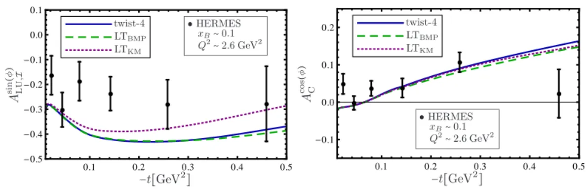
the helicity amplitudes for all possible polarization combinations is performed within the framework of QCD operator product expan- sion. As a result the known accuracy of the amplitudes is improved to include the (kinematic) twist-4 contributions. For the most part the analysis focuses on spin-1/2 targets, the answers for scalar targets conveniently emerge as a byproduct. We investigate the analytical structure of these corrections and prove consistency with QCD fac- torization. We give an estimation of the numerical impact of the sub-leading twist contributions for proton targets with the help of a phenomenological model for the nonperturbative proton gene- ralized parton distributions. We compare different twist approxima- tions and relate predictions for physical observables to experiments performed by the Hall A, CLAS, HERMES, H1 and ZEUS collabora- tions. The estimate also includes a numerical study for planned COMPASS-II runs. Throughout the analysis special emphasis is put on the convention dependence induced by finite twist truncation of scattering amplitudes.
Björn Michael Pirnay
Higher twist effects in deeply virtual Compton scattering
Herausgegeben vom Präsidium des Alumnivereins der Physikalischen Fakultät:
Klaus Richter, Andreas Schäfer, Werner Wegscheider
Dissertationsreihe der Fakultät für Physik der Universität Regensburg, Band 50
Dissertation zur Erlangung des Doktorgrades der Naturwissenschaften (Dr. rer. nat.) der naturwissenschaftlichen Fakultät II - Physik der Universität Regensburg
vorgelegt von Björn Michael Pirnay aus Regensburg im Jahr 2014
Die Arbeit wurde von Prof. Dr. V. M. Braun angeleitet.
Das Promotionsgesuch wurde am 28.05.2014 eingereicht.
Prüfungsausschuss: Vorsitzender: N. N.
1. Gutachter: Prof. Dr. V. M. Braun 2. Gutachter: Prof. Dr. A. Schäfer weiterer Prüfer: N. N.
Björn Michael Pirnay
Higher twist effects in deeply
virtual Compton scattering
in der Deutschen Nationalbibliografie. Detailierte bibliografische Daten sind im Internet über http://dnb.ddb.de abrufbar.
1. Auflage 2016
© 2016 Universitätsverlag, Regensburg Leibnizstraße 13, 93055 Regensburg Konzeption: Thomas Geiger
Umschlagentwurf: Franz Stadler, Designcooperative Nittenau eG Layout: Björn Michael Pirnay
Druck: Docupoint, Magdeburg ISBN: 978-3-86845-135-1
Alle Rechte vorbehalten. Ohne ausdrückliche Genehmigung des Verlags ist es nicht gestattet, dieses Buch oder Teile daraus auf fototechnischem oder elektronischem Weg zu vervielfältigen.
Contents
1. Introduction 7
2. Conventions and light-cone formalism 11
3. Aspects of the operator product expansion 15
3.1. Formulation of the problem . . . 15
3.2. Operator product expansion to kinematic twist-4 accuracy . . . 19
3.2.1. Twist-2 . . . 21
3.2.2. Twist-3 . . . 21
3.2.3. Twist-4 . . . 21
3.3. On gauge invariance and translations . . . 22
4. Deeply virtual Compton scattering 25 4.1. Basics . . . 25
4.2. Helicity amplitudes . . . 28
4.3. Generalized parton distributions in a nutshell . . . 32
5. Calculation of helicity amplitudes 39 5.1. Notation . . . 39
5.2. Transverse helicity flipA±∓ . . . 40
5.2.1. Twist-2 . . . 40
5.2.2. Twist-3 . . . 42
5.2.3. Summary . . . 44
5.3. Longitudinal-to-transverse helicity flipA0± . . . 44
5.3.1. Twist-2 . . . 44
5.3.2. Twist-3 . . . 45
5.3.3. Summary . . . 46
5.4. Helicity conserving amplitudesA±± . . . 46
5.4.1. Difference termδA . . . 48
5.4.2. Trace part ATr . . . 49
5.4.3. Helicity difference ∆A . . . 56
6. Discussion of the results 59 6.1. GPD expressions . . . 59
6.2. Analyticity . . . 61
6.2.1. On factorization . . . 61
6.2.2. Dispersion relations . . . 63
6.3. A byproduct: pion DVCS . . . 66
6.4. Comparison with existing results . . . 67
6.4.1. On the relation to Ref. [15] and the large-Q2limit . . . 67
6.4.2. On the relation to Ref. [40] – twist-3 and partial twist-4 . . . 68
6.5. Compton form factors . . . 71
7. Phenomenology: confronting physical observables 77
7.1. A different CFF basis: BMJ formulation . . . 77
7.2. Model and conventions . . . 80
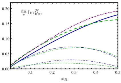
7.3. Impact of power corrections in DVCS . . . 84
7.3.1. Preliminaries . . . 84
7.3.2. Fixed target, unpolarized . . . 85
7.3.2.1. Beam spin sum/difference . . . 85
7.3.2.2. Asymmetries . . . 88
7.3.3. Fixed target, polarized . . . 90
7.3.4. Collider experiments . . . 92
8. Conclusions and outlook 95
A. The leading twist projector in practice 97
B. Fourier transformation cheat sheet 101
C. From DDs to GPDs 103
1. Introduction
Understanding the internal structure of nucleons in terms of its underlying degrees of freedom – quarks and gluons – is a fundamental challenge to be addressed in quantum chromody- namics (QCD). An answer to this problem seems to be very elusive and today our picture is still far from complete.
Experimental activities on this subject began more than 50 years ago and are still ongo- ing. The cornerstone experiments started with the measurements by McAllister and Hof- stadter [1], who determined the form factors of the proton and established its finite size.
These findings triggered further interest in the substructure of the proton both from ex- perimental and theoretical side. In early attempts, Gell-Mann and Zweig [2, 3] proposed a model of quarks which build up hadronic matter. It had to be clarified if quarks were just a mathematical “trick” or actual particles. Progress came later through the first mea- surements ondeep inelastic scattering (DIS) at SLAC [4,5], which pioneered further insight into the inner workings of a nucleon. The observed agreement with theBjorken scaling [6]
of the structure functions supported the mechanism that the scattering occurs off almost free point-like constituents, calledpartons. From today’s theoretical perspective the partons are identified with the QCD building blocks, quarks and gluons. Violation of the Bjorken scaling behavior was predicted from QCD [7,8] and found later [9], providing an important test of the theory. DIS along with many other experiments established QCD as the accepted theoretical framework for hadronic matter.
Extracting predictions from QCD itself is in general a nontrivial problem. One reason for this is the intrinsic limitation of the applicability of perturbative methods. Perturbation theory works at high energies (or short distances) but it breaks down at small energies (long distances) through the running coupling constantαs(Q2) [10,11]. Among the established nonperturbative approaches to the low energy sector of the theory, numerical methods from first principles based on lattice formulations of QCD seem to be the most promising. Most observables, e.g. cross sections, are a mixture of both long- and short-distance effects. A separation between the two domains is established by factorization theorems. Observables (in a general sense including amplitudes etc.) are written as products or convolutions of hard scattering coefficients, calculable in a perturbative framework, with phenomenological but universal nonperturbative functions. This approach necessarily introduces a factorization scale and the dependence of the two “factors” on it can be studied by renormalization group methods or evolution equations. The driving evolution kernels can be calculated order by order in perturbation theory. The nonperturbative input is a priori unknown, but one can revert to a phenomenological treatment and extract it from experimental data, usually by means of a suitable model or parametrization. In the case of DIS these are the parton distribution functions (PDFs), describing the probability densities to find a certain parton with a given longitudinal momentum and polarization inside a fast moving nucleon.
Universality guarantees that, once determined from one set of measurements, the PDFs can be used to describe any other experiment to which they contribute.
More rigorously, in the sense of a quantum field theory, the PDFs are defined by forward matrix elements of nonlocal twist-2 light-ray operators bilinear in quark or gluon fields.
Such PDFs contain some, but certainly not all information about the nucleon substructure.
They are, by definition, restricted to the longitudinal degree of freedom and insensitive
to multi-particle correlations. PDFs should rather be regarded as one of many aspects of the nucleon landscape, determining its global shape. In principle, a complete “nucleon map”, would require the knowledge of the whole nucleon wave function, including infinitely many Fock components. At present, a theoretical solution to this bound state problem in QCD is out of reach. Instead one tries to view the nucleon from different “angles” by considering generalizations of PDFs or operators that encode more or different feedback from the nucleon. Necessarily there should be at least one experiment sensitive to such extensions.
One of the most prominent concepts that emerged in the last two decades is that of generalized parton distributions(GPDs), defined in [12–14]. Excellent reviews on the subject can be found in Refs. [15,16]. The distinction from the ordinary PDFs is simple: instead of taking the forward matrix element of the light-ray operators, sayhp|. . .|pi, one considers the off-forward one,hp0|. . .|pi, with two, possibly different, momentum eigenstates of the hadron.
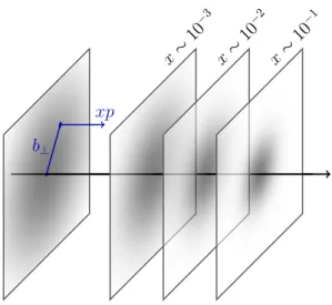
In addition to the usual PDF variablesxandQ2GPDs now depend on two more variables, the squared momentum transfer t = (p−p0)2 and the skewness ξ, which is essentially a longitudinal fraction of the momentum difference. This innocent-looking generalization opens a wide door into the nucleon landscape. Two of the “hot topics” that can be accessed within GPDs shall not go unmentioned. Already in early developments, Ji [17] realized that certain moments of GPDs are related to the nucleon energy momentum tensor (or better yet a particular version of it). Thus they can be used to quantify how the spin and orbital angular momentum is distributed among quarks and gluons. There are several subtleties about this decomposition, being actively debated to the present day, see Ref. [18] for a recent review. Apart from that, it was shown later [19,20], that GPDs provide a valuable source of information about the momentum distribution of partons, that goes beyond the usual collinear PDF description and allows one to access a three-dimensional spatial image of the nucleon. Through the so-called impact parameter representations, GPDs encode a probabilistic distribution of partons in the plane transverse to the nucleon’s direction of motion (in the infinite momentum frame) as a function of the distance from the nucleon’s center. The picture, which was originally formulated at zero skewness, was refined later [21]
and shown to hold also for nonzeroξ(with a change of the center of transverse momentum interpretation).
Constraints on GPDs arise through the observation that some of the “old” key observables in hadron physics are naturally contained in them. Most importantly, DIS constrains those GPDs, which allow a reduction to the usual PDFs in the limitξ→0,t→0 or p0→p. Fur- ther requirements come from certain Mellin moments inx, the first moments being related to the elastic form factors and the anomalous magnetic moment. The second moments enter directly in Ji’s spin sum rule [17].
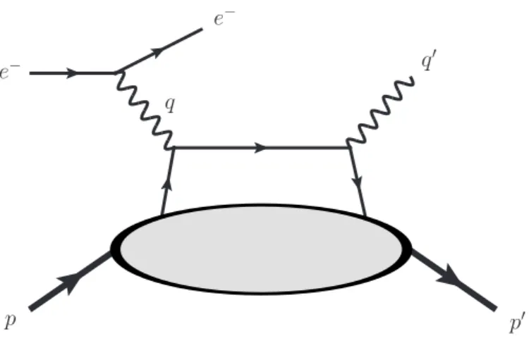
Having established the physical significance of GPDs, one realizes that they are probed, apart from the aforementioned limiting cases, in hard exclusive reactions with nonzero mo- mentum transfer. The bulk of experimental data comes fromdeeply virtual meson production anddeeply virtual Compton scattering (DVCS). The latter, which is also the main topic of this work, is defined as the process where a photon of high virtualityQ2scatters off a nucleon with emission of a real photon in the final state. It appears as part of the leptoproduction of a photon off a nucleon and is regarded as the cleanest reaction channel to access GPDs.
Factorization for this process has been proven in the limit of largeQ2 [22]. In reality many of the existing and future measurements lie somewhere in the ballpark ofQ2∼2−15 GeV2. Naturally, an analysis of the subleading corrections in 1/Qis important.
The theoretical description for DVCS relies on theoperator product expansion (OPE) of the time-ordered product of two electromagnetic quark currents. Suppressed contributions originate from higher twist operators in this framework. Here we focus on a particular
subset of 1/Q-effects, dubbedkinematic power corrections [23,24]. They are analogous to the so-calledNachtmann corrections [25] in DIS, which stem from the “subtraction of traces”
prescription for the leading twist operators. For DVCS one faces additional complications since the contributions of total derivatives of the twist-2 operators have to be included as well. In DIS they are absent, since matrix elements of total derivatives are proportional to the momentum differences of the initial and final state. The technically demanding operators are those of the form (∂O) = ∂µOµµ1...µn, where Oµµ1...µn is a local (conformal) quark- antiquark leading twist operator. Due to a theorem by Ferrara et al. [26] (∂O) vanishes in the free field theory. By QCD equations of motion in the interacting theory one can relate (∂O) to three-particle quark-antiquark-gluon operators, which appear (among others) in the OPE at twist-4 level. The separation of contributions proportional to (∂O) from the OPE is a very involved algebraic task and has been solved only recently [23,24]. Parts of this thesis are based on these results. In the kinematic approximation one considers only the leading twist descendants and neglects the “genuine” multi-particle correlations in the target, i.e. those that are not related to the leading twist operators by QCD equations of motion. By definition this does not introduce any (new) nonperturbative input apart from the GPDs themselves. As a consequence we are able to compute the DVCS process amplitudes including mass (m2/Q2) and momentum transfer (t/Q2) corrections. The latter are of particular relevance, given the fact that for the three-dimensional imaging of the nucleon, a sufficiently broad interval in|t|, maybe up to 2 GeV2[27], needs to be covered by experiments. Note that it is a priori not clear whether factorization still holds for the power corrections and we shall address this question.
The presentation is organized as follows: In the next chapter we briefly spell out our conventions and necessary notations. Chapter 3 reviews key features of the operator product expansion to (kinematic) twist-4 accuracy, in particular relevant contributions to off-forward reactions. The prime reaction of interest, deeply virtual Compton scattering, is introduced in Chapter 4 along with its kinematics, amplitudes and the ever present generalized parton distributions and their parametrizations in terms of double distributions. The latter form a convenient foundation for the calculation of helicity amplitudes. We outline technical details and intermediate expressions in Chapter 5. Further processing of the results is presented in Chapter 6, investigating their properties and giving several equivalent representations.
By selecting a popular GPD model, the phenomenological impact is examined in Chapter 7 through a comparison with leading twist conventions and available experimental data on several representative observables. Finally we conclude in Chapter 8 and outline further possible applications. In addition we include the Appendices A, B and C, where technical questions of general relevance for this work are addressed.
2. Conventions and light-cone formalism
For this work it is of utmost importance to specify the conventions of special relativity. We devote this chapter to a detailed and hopefully unambiguous presentation of the notation.
It may serve as a reference for future applications.
Our choice of the metric tensor of the Minkowski space has a “mostly negative” signature,
gµν
=
1 0 0 0
0 −1 0 0
0 0 −1 0
0 0 0 −1
. (2.1)
For theγ-matrices we use theWeyl representation, γ0=γ0=
0 1 1 0
, γi=−γi=
0 σi
−σi 0
, γ5=iγ0γ1γ2γ3=
−1 0
0 1
, (2.2) whereσi, i= 1,2,3 are the three Pauli matrices,
σ1= 0 1
1 0
, σ2=
0 −i i 0
, σ3= 1 0
0 −1
. (2.3)
The definition ofγ5 can equivalently be written as γ5= i
4!εµνρσγµγνγργσ, ε0123= 1, (2.4) occasionally known as theBjorken-Drell convention [28].
With the form (2.2) of theγ-matrices the generators of the Lorentz group σµν = i
2[γµ, γν] (2.5)
are 2×2 block-diagonal. This already implies that a Dirac spinor q does not transform according to an irreducible representation of the Lorentz group. The 2×2 blocks cannot be diagonalized further, essentially because the Pauli matrices do not admit it. Therefore a Dirac spinor is an element of the direct sum of two irreducible representations, which are often dubbed (1/2,0) and (0,1/2), each of dimension two. By Hermitian conjugation of (1/2,0) one gets a representation that is equivalent to (0,1/2). We write a Dirac spinor q as
q= ψα
¯ χα˙
, (2.6)
where the two-component objectsψα, ¯χα˙, which transform according to an irreducible rep- resentation of the Lorentz group, are calledWeyl spinors. They correspond to the left- and right-handed projections of q respectively. To distinguish the respective chirality, we use dotted and undotted indices for the components of the Weyl spinors. The Dirac-adjoint
spinor ¯q=q†γ0 is
¯
q= χα,ψ¯α˙
, χα= ¯χα˙†
, ψ¯α˙ = ψα†
. (2.7)
In that context it is necessary to define raising and lowering of spinor indices, which is done with the help of the two-dimensional Levi-Civita symbol
uα=εαβuβ, uα=εβαuβ, u¯α˙ =εβ˙α˙u¯β˙, u¯α˙ =εα˙β˙u¯β˙, (2.8) for arbitrary Weyl spinorsuα,u¯α˙. The convention forεis as follows:
ε12=ε12= 1, ε21=ε21=−1,
ε2 ˙˙1=ε2 ˙˙1= 1, ε1 ˙˙2=ε1 ˙˙2=−1. (2.9) Note that indeed Eqs. (2.8), (2.9) guarantee that raising followed by lowering of an index (or vice versa) is the identity operation. Quite frequently one encounters the contraction of two Weyl spinors, for which we introduce a shorthand notation, The convention adopted here follows an “up-down” rule for undotted and a “down-up” rule for dotted indices, i.e.
(uv) =uαvα, (¯u¯v) = ¯uα˙v¯α˙ , (2.10) which is different in sign compared to the reversed case, i.e.
(vu) =−(uv), (¯vu) =¯ −(¯u¯v). (2.11) As a trivial example consider the scalar combination ¯qqwhereqand ¯qare the Dirac spinor and its adjoint, then
¯
qq= (χψ) + ( ¯ψχ)¯ . (2.12)
The usual Lorentz vectors are also incorporated in this formalism by the following con- struction: One uses the 2×2 unit matrix1and the three Pauli matrices to map the vector xµto 2×2 matrices (x) =xµσµ withσµ= (1, ~σ) and (¯x) =xµσ¯µ with ¯σµ= (1,−~σ), which take the form
xαα˙
=xµ σµ
αα˙ =
x0+x3 x1−ix2
x1+ix2 x0−x3
,
¯ xαα˙
=xµ σ¯µαα˙
=
x0−x3 −x1+ix2
−x1−ix2 x0+x3
. (2.13)
The “first” index always refers to the row and the second index to the column of the matrix, e.g. x1 ˙2 =x1−ix2 =−¯x12˙ . In the conventional light-cone formalism the diagonal entries correspond to the “plus” and “minus” projections on the light-cone. The components trans- verse to it are encoded in the off-diagonal holomorphic and anti-holomorphic (in x1, x2) entries. Ifxµis a real-valued vector, then the matrices (xαα˙) and (¯xαα˙ ) are Hermitian. The Minkowski scalar product of two vectorsxµ andyµ can be written as half of the trace of the product of one “barred” and one “unbarred” matrix
(xy) =1
2xαα˙y¯αα˙ . (2.14)
Raising and lowering of spinor indices works just as in the spinor case, e.g.
xαα˙ =εαβxββ˙εβ˙α˙ = ¯xαα˙ . (2.15) In practical calculations the Fierz identities for Pauli-matrices come in handy:
(σµ)αα˙(¯σµ)ββ˙ = 2δβαδβα˙˙, (σµ)αα˙(σµ)ββ˙ =−2εαβεα˙β˙. (2.16) Ifxµ is a real-valued Lorentz vector, then its associated matrix obeys
(x†)αα˙ = ¯xαα˙ . (2.17)
Note that the above formulation for vectors generalizes trivially to any Lorentz tensor, i.e.
a Lorentz tensor of rankn, say tµ1···µn, is mapped to a spinorial tensor with ndotted and nundotted indices,
tα1α˙1···αnα˙n ≡σαµ1
1α˙1· · ·σµαn
nα˙ntµ1···µn. (2.18) A nice collection of helpful formulas on this particular topic is provided in Ref. [29], however one should keep in mind that [29] uses partially different conventions compared to this work.
In some situations it is useful to have explicit representations for the solutions of the free Dirac equation (/p−m)uλ(p) = 0, (/p+m)vλ(p) = 0 with massmand helicityλ. Our choice corresponds to [30]
u↑(p) = 1 pp0+p3
m
0 p0+p3 p1+ip2
, u↓(p) = 1 pp0+p3
ip2−p1 p0+p3
0 m
,
v↑(p) = 1 pp0+p3
ip2−p1 p0+p3
0
−m
, v↓(p) = 1 pp0+p3
−m 0 p0+p3 p1+ip2
, (2.19)
and implies the normalization conditions ¯uλ(p)uλ0(p) = 2mδλλ0, ¯vλ(p)vλ0(p) = −2mδλλ0. The helicity labels refer to the eigenvalues of the spin projection along the momentum for a particle moving fast in the negativez-direction. In more detail, the helicity operatorh∞in this infinite momentum frame reads [30]
h∞(p) = 1 2
1 2pp10−ip+p32 0 0
0 −1 0 0
0 0 1 0
0 0 2pp10+ip+p32 −1
, (2.20)
and is diagonalized byu↑,↓(p),v↑,↓(p), h∞(p)u↑(p) = +1
2u↑(p), h∞(p)u↓(p) =−1 2u↓(p), h∞(p)v↑(p) =−1
2v↑(p), h∞(p)v↓(p) = +1
2v↓(p). (2.21)
3. Aspects of the operator product expansion
3.1. Formulation of the problem
In many physical applications where some hadronic system is probed by electromagnetic interactions, observables are parametrized in terms of products of electromagnetic currents constructed from quark fields. Examples include the e+e− annihilation into hadrons, the famous deep inelastic scattering and, most relevant here, Compton scattering. For our purposes the goal is to study the behavior of the time-ordered product of two currents
Tµν =iT
jµ(z1x)jν(z2x) . (3.1)
Here z1 and z2 are some real numbers, their role will be discussed later. The current is defined as
jµ(x) = ¯q(x)γµq(x). (3.2)
For simplicity we consider just one quark flavor, and the summation over equal colors,
¯
q(x)γµq(x) ≡q¯i(x)γµqi(x), is left implicit. Hard processes are dominated from regions of Tµν near the light-cone x2 →0. A technical complication arises since the product of fields at light-like distances is ill-defined in general due to a singular behavior in 1/x2. Simple examples can be constructed e.g. in the free field theory. To make this more tractable Wil- son [31] proposed a Laurent-like series for products of fields with possibly singular coefficient functions and regular operators, called operator product expansion. A formal proof of the OPE was given later by Zimmermann [32].
Following [33], let us review heuristically how the OPE works in practice. The T-product consists of four fermionic operators. According to the Wick theorem, one can rewrite it in terms of all possible products of contractedq¯qfields with the remaining uncontracted fields in normal order. For the scattering processes which we are going to consider, we can ignore disconnected Feynman diagrams. The contributions where all fields are contracted would correspond to one of those and can be disregarded for our purposes. The leading singular (in 1/x) terms are extracted by contracting two of the quark fields and leaving the remaining two uncontracted:
Tµν =i q(z¯ 1x)γµq(z1x)¯q(z2x)γνq(z2x) + ¯q(z1x)γµq(z1x)¯q(z2x)γνq(z2x) +. . .
. (3.3) A contribution of all fields left uncontracted also exists, but it is not singular as x2 → 0 and can be neglected. In the leading order the contractionq(z1x)¯q(z2x) is the (massless) propagator of a quark in coordinate representation
q(z1x)¯q(z2x) = i/x
2π2(z12)3(x2−i0)2 +. . . . (3.4)
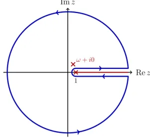
Again the notation is kept short here, suppressing explicit Dirac indices and a unit matrix in color space. In the above formula, the “i0” stands for “i times an infinitesimal positive number” and corresponds to Feynman’s causality prescription. In the following we will leave it implicit, whenever its appearance is unimportant. We also use the following abbreviation
z12=z1−z2. (3.5)
Including the correction to the first order in the couplingg one gets, cf. [33]
q(z1x)¯q(z2x) = i/x 2π2(z12)3x4 +
Z
d4y i(z1/x−/y)
2π2(z1x−y)4ig /A(y) i(/y−z2/x)
2π2(y−z2x)4 +. . . . (3.6) The color structure in the second term is contained in the field (A(y))/ ij ≡TijaA/a(y), when i and j are the color indices of q(z1x) and ¯q(z2x) respectively. Tija are the generators of the color gauge group SU(3) in the fundamental representation with i, j ∈ {1,2,3} and a∈ {1, . . .8}. To make progress on this term
∆G(z1x, z2x)≡ Z
d4y i(z1/x−/y)
2π2(z1x−y)4ig /A(y) i(/y−z2/x)
2π2(y−z2x)4 (3.7) we introduce the Feynman parametrization to combine the two denominators and shift the y-integration byy→y+z21uxto cast it into the form
∆G(z1x, z2x) =−ig 3 2π4
Z 1 0
du uu¯ Z
d4y(z12u/¯x−/y)A(y/ +z21ux)(/y+z12u/x)
[y2+u¯u(z12x)2]4 , (3.8) where
zu21= ¯uz2+uz1, u¯= 1−u . (3.9) Since we want to study the behavior of Tµν at small distances x, we expand the gauge field aroundy= 0,
A(y/ +z21ux) =A(z/ 21ux) + (y∂)A/
(z21ux) +. . . , (3.10) from which we obtain
∆G(z1x, z2x) =−g /x 2π2(z12)2x4
Z 1 0
du(xA)(zu21x)
− g 8π2z12x2
Z 1 0
du(¯u/xγµγν−uγνγµx)(∂/ νAµ)(z21ux) +. . . . (3.11) Here the ellipses stand for terms of higher order inx. In deriving Eq. (3.11), we utilized the integrals
Z
d4y 1
(−y2+z2+i0)n =−iπ2Γ(n−2) Γ(n)
1 (z2+i0)n−2, Z
d4y yµyν
(−y2+z2+i0)n = +iπ2Γ(n−3) 2Γ(n)
gµν
(z2+i0)n−3. (3.12) Note that in the Taylor expansion ofA(y+zu21x), Eq. (3.10), higher order terms iny would
3.1. FORMULATION OF THE PROBLEM
always produce suppressed, less singular, contributions in x. The first term in Eq. (3.11) together with the leading order expression forms the first order in g of the path-ordered exponential,
[z1x, z2x] = Pexp
ig Z 1
0
du z12(xA)(z21ux)
≡
∞
X
n=0
(iz12g)n Z 1
0
du1 Z u1
0
du2· · · Z un−1
0
dun(xA)(zu211x)· · ·(xA)(zu21nx). (3.13) Its role is to restore gauge invariance for the remaining fields at different points. Note that the order of the gauge fields in (3.13) is important, sinceAis matrix-valued.
For simplicity we employ the Fock-Schwinger gauge, which is defined by the condition
(xA)(x) = 0, Aµ(0) = 0. (3.14)
From these two requirements follows a simple integral representation of the gauge fieldAµin terms of the field strength tensorFµνa =∂µAaν−∂νAaµ+gfabcAaµAbν (the structure constants of SU(3) arefabc=−2iTr [Ta, Tb]Tc
), Aµ(x) =
Z 1 0
dα αxνFνµ(αx), Aµ=AaµTa, Fµν =Fµνa Ta. (3.15) In this gauge the path-ordered exponential reduces to unity. Further, by using the above formula and the equation of motion, the total divergence (∂A) is of order g. This, along with theγ-matrix identity
γαγµγν =gαµγν+gµνγα−gανγµ−iγ5γρεραµν (3.16) allows us to rewrite our expression for the propagator in terms ofFµν andFeµν = 12εµνρσFρσ,
q(z1x)¯q(z2x) = i/x
2π2(z12)3x4 + g 8π2z12x2
Z 1 0
du xµγν
(¯u−u)Fµν(z21ux)−iγ5Feµν(z21ux) , (3.17) up to higher order corrections inxand g. To the same accuracy one readily reads off the expansion of the time-ordered product, Eq. (3.3):
Tµν=Tµν(a)+Tµν(b)+ µ↔ν, z1↔z2
, (3.18)
with
Tµν(a)=− 1
2π2(z12)3x4q(z¯ 1)γµxγ/ νq(z2), Tµν(b)= g
8π2z12x2 Z 1
0
duq(z¯ 1)γµxργσ
i(¯u−u)Fρσ(z21u) +γ5Feρσ(z21u)
γνq(z2), (3.19) where we have introduced a shorthand notation for the arguments of the fields,
¯
q(z1)≡q(z¯ 1x) etc., (3.20) leaving the dependence on the space-time point x implicit. A manifestly gauge invariant
form of Eqs. (3.19) is obtained by restoring the proper gauge links between the fields. The expressions (3.19) can be viewed as the starting point of the calculation in Ref. [23]. In order to systematically classify contributions toTµν according to their importance (or better yet their power behavior) in the scattering amplitudes, one needs to order the contributions by their twist.
The leading twist part is isolated fromTµν(a)by symmetrization and trace subtraction on the level of local operators. Here only operators bilinear in the quark fields appear and they will ultimately result in a GPD description of the scattering process (to this accuracy). This is technically not very demanding and can be done within a couple of lines of algebra, cf. [23].
Once one starts to include subleading twist contributions it becomes more complicated.
Starting at twist-3 one encounters derivatives of twist-2 operators as well as operators with an additional gluon field. They may be related by equations of motion. Let us consider a simple example by taking the operator (in the convention of Eq. (3.20))
¯
q(z1)γµq(z2). (3.21)
as well as the Fock-Schwinger gauge (3.15), then one obtains
∂ν q(z¯ 1)γµq(z2)
=z1[ ¯Dνq](z¯ 1)γµq(z2) +z2q(z¯ 1)γµ[Dνq](z2) +igz12
Z 1 0
du z21uq(z¯ 1)xρFρν(zu21)γµq(z2), (3.22) where
Dµ=∂µ−igAaµTa,
D¯µ=∂µ+igAaµ(Ta)t. (3.23) Although rather schematic, the above equation (3.22) is an example of the entanglement of a total derivative of a two-particle operator with a higher twist operator containing more fields, as present in Tµν(b). Apart from the explicit appearance of ¯qF q-type operators in Tµν(b), they also appear implicitly inTµν(a), starting from twist-3. The lesson to be learned is that operators of the type ¯qF q do not necessarily give rise to genuine higher twist multi- particle correlations, but contain descendants of the leading twist operators. The latter are relevant for the power corrections in hard exclusive processes and one would like to have them separated from the dynamical higher twist sector. Such a separation is feasible because the dynamical orquasipartonicoperators obey an autonomous set of renormalization group equations. Putting them to zero at one scale ensures that they do not reappear at another scale.
The separation of the contributions of interest turns out to be surprisingly difficult. In Refs. [23,24] this problem has been addressed and solved. A helpful input that went into this calculation was the renormalization group of twist-4 operators at one-loop accuracy, cf. [34,35]. The operators that are relevant for the power corrections fall into the class of so-callednonquasipartonic operators. One of the major results given in [34,35] was the proof that there exists a certain scalar product for the quasipartonic sector, which has the property that the matrix of anomalous dimensions is Hermitian w.r.t. this product. This feature was identified to be a consequence of conformal invariance of massless QCD at one-loop order.
Hermiticity implies orthogonality of the anomalous dimension eigenvectors. It was shown that this property is sufficient to separate the relevant contributions, thus bypassing the direct diagonalization of the renormalization kernels, which is probably a very difficult task.
Of course, for this approach to work in practice the explicit knowledge of the scalar product
3.2. OPE TO KINEMATIC TWIST-4 ACCURACY
is necessary which is also available in [34,35]. The actual derivation is then basically reduced to an algebraic problem and can be found in [23]. We will merely quote the results and take the opportunity to introduce necessary notation.
3.2. Operator product expansion to kinematic twist-4 accuracy
The results of [23] are most conveniently presented in the spinor formalism, see Ch. 2. To this end we write for the time-ordered product
Tααβ˙ β˙ =iT
jαα˙(z1x)jββ˙(z2x) , (3.24) and its expansion to the order 1/x2 can be cast into the form
Tααβ˙ β˙ =− 2 π2(z12)3x4
h
xαβ˙Bβα˙(z1, z2)−xβα˙Bαβ˙(z2, z1) +xαβ˙xβα˙ A(z1, z2)−A(z2, z1) +x2 xββ˙∂αα˙C(z1, z2)−xαα˙∂ββ˙C(z2, z1)i
. (3.25)
Here the derivative∂αα˙ =∂µ(σµ)αα˙ acts w.r.t. the space-time pointx. The operatorsA, C are pure twist-4 corrections and B is a sum of all twists from two to four, which we conveniently label by
Bαα˙(z1, z2) =Bt=2αα˙ (z1, z2) +Bt=3αα˙ (z1, z2) +Bt=4αα˙ (z1, z2). (3.26) Explicit expressions forA,B,Cwill be given below, after a couple of preparatory definitions.
First we define the vector and axial-vector operators OV(z1, z2) = ¯q(z1x)/xq(z2x),
OA(z1, z2) = ¯q(z1x)/xγ5q(z2x), (3.27) as well as their (anti-)symmetrized versions
OV,−(z1, z2) =OV(z1, z2)− OV(z2, z1),
OA,+(z1, z2) =OA(z1, z2) +OA(z2, z1). (3.28) It is necessary to have a projection ofO...on leading twist operators. To this end one makes use of a (real) auxiliary light-like vectorn, which can always be represented with the help of two spinorsλ,λ¯
nµ=12(σµ)αα˙λα¯λα˙ , n2= 0, (3.29) with ¯λ= λ†, see Ch. 2. Completely equivalent is of course nαα˙ =λα¯λα˙. The particular combination of axial and vector operators that will enter in the OPE is denoted by
O++(z1, z2) = ¯ψ+(z1n)ψ+(z2n)−χ+(z2n) ¯χ+(z1n), (3.30)
where
ψ+=λαψα, ψ¯+= ¯λα˙ψ¯α˙ ,
χ+=λαχα, χ¯+= ¯λα˙χ¯α˙. (3.31) Note thatO++(z1, z2) itself is twist-2 and it is equivalent to
O++(z1, z2) = 1 2
OV,−(z1, z2)− OA,+(z1, z2)
x→n. (3.32)
The separation of the leading twist contributions from O... as function of x, which is not light-like, is achieved by the leading twist projector Π. Let ϕ(x) be an arbitrary operator andϕ(λ,λ) its restriction on the light-ray¯ n, expressed in terms of λ,¯λ. Then Π is defined as follows:
[Πϕ](x) = Π(x, λ)ϕ(λ,λ) =¯
∞
X
k=0
( ¯∂¯x∂)k
(k!)2 ϕ(λ,¯λ)
λ=¯λ=0, (3.33) where
( ¯∂x∂) =¯ ∂
∂¯λα˙x¯αα˙ ∂
∂λα. (3.34)
The application of the leading twist projection to any operator will be denoted by the superscript “t= 2”, e.g.
Ot=2++(z1, z2) = Π(x, λ)O++(z1, z2). (3.35) Technically, Π implements the symmetrization and subtraction of traces for the Lorentz indices in each coefficient in the Taylor expansion ofO++(z1, z2). Since the nonlocal operator O++(z1, z2) can be interpreted as the generating function for local operators, one may think of [ΠO++](z1, z2) as the generating function for local twist-2 operators. To see that [ΠO++](z1, z2) has the desired properties, consider the k-th term in the expansion (3.33).
It reads 1
(k!)2x¯α˙1α1· · ·x¯α˙kαk ∂
∂λ¯α˙1· · · ∂
∂λ¯α˙k
∂
∂λα1· · · ∂
∂λαkO++(z1, z2)
λ=¯λ=0. (3.36) The tensor
∂
∂λ¯α˙1· · · ∂
∂¯λα˙k
∂
∂λα1 · · · ∂
∂λαkO++(z1, z2) (3.37) is symmetric under an arbitrary exchange of two dotted or two undotted indices. Therefore it is also symmetric under the simultaneous exchange of two pairs of indices (αi,α˙i)↔(αj,α˙j).
Interchanging two such pairs in this way is equivalent to the interchange of two Lorentz indices in the usual vector formalism. Tracelessness is also easy to see, since taking a trace with respect to two Lorentz indices corresponds to the contraction with a dotted and an undottedε-symbol.
The upcoming calculations can become rather cumbersome, if one insists on using the very definition of Π in Eq. (3.33). In App. A we give a proof of a simpler representation of Π accurate to the orderx2, to which all calculations are done. It shall be stressed here, that this is only for convenience and using Eq. (3.33) directly is also possible. However, as
3.2. OPE TO KINEMATIC TWIST-4 ACCURACY
repeatedly pointed out in [23], translation and gauge invariance is only guaranteed to work at twist-4 level, see also Sec. 3.3, thus there is no real need to cope with the “full” expression of Π.
With these preliminaries we can now proceed to give explicit formulas for (3.25) and (3.26).
3.2.1. Twist-2
The twist-2 contribution to the OPE is entirely contained in Bαα˙, see Eq. (3.26), and is given by
Bt=2αα˙ (z1, z2) =1 2∂αα˙
Z 1 0
duO++t=2(uz1, uz2). (3.38) It originates from the leading twist projection ofTµν(a)in Eq. (3.19).
3.2.2. Twist-3
In this sector we have Bt=3αα˙ (z1, z2) = 1
4 Z 1
0
du u Z z1
z2
dv z12
n
z1 (x¯σµ∂)αα˙ + lnu ∂αα˙x2∂µ
iPµ,Ot=2++(uz1, uv) +z2 (¯xσµ∂)¯αα˙ + lnu ∂αα˙x2∂µ
iPµ,Ot=2++(uv, uz2)o , (3.39) where [Pµ, . . .] stands for the commutator with the momentum operatorPµ. If one evaluates this operator in the basis of momentum eigenstates, one may simply replace [Pµ, . . .] by the difference of eigenmomenta between final and initial state. Note that the contributions
∼ lnu are twist-4 terms, whose role is to subtract twist-4 contaminations from the rest, such thatBt=3αα˙ is purely twist-3.
3.2.3. Twist-4
Let us now give the twist-4 contributions,A, Bt=4αα˙ andC. Out of the multitude of equiv- alent representations that are given in [23], we will pick the most convenient one for our calculations.
The termA(z1, z2), entering antisymmetrized inz1↔z2, reads A(z1, z2) =1
4 Z 1
0
du
z1z2u2lnuO1(uz1, uz2) +
z2∂z2− z1
z12
−lnu z2∂z22z12
R(uz1, uz2)
−
z1∂z1− z2 z21
−lnu z1∂z2
1z21
R(uz¯ 1, uz2)
, (3.40)
with
R(z1, z2) =z12
Z z1 z2
dv z12
Z v z2
dw z12
w−z2
z1−w 1
2S+O1(v, w)−(S0−1)O2(v, w)
, R(z¯ 1, z2) =z12
Z z1 z2
dv z12
Z v z2
dw z12
z1−v v−z2
1
2S+O1(v, w)−(S0−1)O2(v, w)
. (3.41) Here the operatorsO1,2are defined as
O1(z1, z2) = iPµ,
iPµ,Ot=2++(z1, z2) , O2(z1, z2) =
iPµ, ∂µOt=2++(z1, z2)
. (3.42)
andS+, S0 are given by
S+=v2∂v+w2∂w+ 2(v+w).
S0=v∂v+w∂w+ 2. (3.43)
Formally, S+, S0 are generators of conformal transformations on the light-ray, acting on products of fields with light-cone positions v, w and conformal spin j = 1, i.e. here S+ ≡ S+(1,1),S0≡S0(1,1)with the general form
S+(j1,j2)=v2∂v+w2∂w+ 2(j1v+j2w),
S0(j1,j2)=v∂v+w∂w+j1+j2. (3.44) The next contribution is
Bt=4αα˙ (z1, z2) =x2∂αα˙Bt=4(z1, z2), (3.45) where
Bt=4(z1, z2) = 1 8
Z 1 0
du u2
u2(1−u2+u2lnu)z1z2O1(uz1, uz2)
−
(1−u2)
z2∂z2− z1
z12
+ (1−u2+u2lnu)z2∂z22z12
R(uz1, uz2) +
(1−u2)
z1∂z1− z2 z21
+ (1−u2+u2lnu)z1∂z2
1z21
R(uz¯ 1, uz2)
. (3.46) Finally the last term reads
C(z1, z2) =−1 8
Z 1 0
du
u2 R(uz1, uz2) + ¯R(uz2, uz1)
. (3.47)
3.3. On gauge invariance and translations
The finite-Q2corrections to the OPE in the case of deep inelastic scattering have first been calculated in [25] and are occasionally calledNachtmann corrections. Technically their origin lies in the “subtraction of traces”-prescription of the leading twist projection. Since DIS can be described by the forward Compton amplitude hp|Tµν|pi, the situation is somewhat
3.3. ON GAUGE INVARIANCE AND TRANSLATIONS
simpler than for off-forward reactions. Forward matrix elements of operators, which are total derivatives, vanish because they are always proportional to the momentum difference between the two proton states. Therefore for DIS the only nonzero contribution stems from Bt=2αα˙ in Eq. (3.38). For the off-forward reactions like DVCS the corrections due to the trace subtraction terms alone are not sufficient, they are in fact unphysical. To see this, we first establish general relations for the time-ordered product of currents.
The tensorTµν(z1, z2) in Eq. (3.1) (here we make the dependence onz1,2explicit) inherits its translational properties from the fundamental fields ¯q(x), q(x), which gives
Tµν(z1+δz, z2+δz) =eiδz(Px)Tµν(z1, z2)e−iδz(Px). (3.48) The infinitesimal version of Eq. (3.48) is
(∂z1+∂z2)Tµν(z1, z2) =
i(Px), Tµν(z1, z2)
. (3.49)
Later, we will give an equivalent relation for (3.48), (3.49) in momentum space. In that framework it can be seen explicitly, that for the Nachtmann-type corrections Eqs. (3.48), (3.49) do not hold. The full translational invariance is only restored when one takes into account all other corrections of twist-3 and twist-4. Eqs. (3.48), (3.49) are then valid up to corrections of twist-5 or higher.
Similarly the (electromagnetic) gauge invariance, which implies current conservation,
∂µjµ(x) = 0, (3.50)
requires
∂µTµν(z1, z2) = T
jµ(z1x)∂µjν(z2x) =z2
iPµ, Tµν(z1, z2) ,
∂νTµν(z1, z2) = T
jν(z2x)∂νjµ(z1x) =z1
iPν, Tµν(z1, z2)
. (3.51)
Here the same subtlety as before arises: The Ward identities (3.51) are fulfilled only in the sum of all twists. This property is known since quite some time and was first noticed in Refs. [36–39] independently.
It can be checked that Eqs. (3.49), (3.51) hold up to corrections of twist-5 or higher.
The condition of gauge invariance will be used from the very beginning when we define the helicity dependent scattering amplitudes. On the other hand the translation property (3.48) will not be exploited at any time. The final result should reflect (3.48) automatically, which provides a very strong check of the calculation, as we shall see below.
4. Deeply virtual Compton scattering
4.1. Basics
Our target application of the OPE formulated in the previous chapter is the deeply virtual Compton scattering. It is defined as the scattering of a virtual photon on a hadron with a real photon in the final state,
h(p) +γ∗(q)→h(p0) +γ(q0). (4.1) Hereq(q0) andp(p0) denote the initial (final) momenta of the participating particles. Their respective polarizations are left implicit. DVCS appears as a subprocess of the exclusive lepton-hadron scattering, see Fig. 4.1. The biggest share of all available experiments on DVCS were performed using protons, and it seems that they will also be the prime target of interest in the foreseeable future. Thus we consider a nucleon target for definiteness, although everything in this work will be valid for any spin-12 baryon. We will comment on the case of scalar targets, e.g. pions, in Sec. 6.3.
At leading order the theoretical description of DVCS is formulated in terms of the hadronic Compton tensor
Aµν =i Z
d4x e−iqxhp0|T
jµ(x)jν(0) |pi. (4.2) On diagrammatic level the photon fields will couple to the Lorentz indicesµ, ν. The scat- tering occurs between the photons and a quark or antiquark being emitted from the proton and reabsorbed in the final state. This is occasionally called the “handbag mechanism”, see Fig. 4.1. Applying the OPE from Ch. 3 to the r.h.s. of (4.2) gives the amplitude tensor in terms of short distance coefficients and nonperturbative input from the proton. This was one of the main tasks in this work, and we will continue to present the essential steps towards the answer in the kinematic twist-4 approximation.
To make progress, we introduce a some conventional notation, starting with kinematical variables. The final state photon is assumed to be real, i.e.
(q0)2= 0. (4.3)
It turns out that instead of working directly with the individual hadronic momentap, p0 it is convenient to introduce the somewhat standard vectorsP and ∆, being the average and difference ofp, p0 respectively,
Pµ=1
2(pµ+p0µ),
∆µ=p0µ−pµ=qµ−q0µ, (4.4) The hard scale of the process is the virtuality of the initial state photon,
Q2=−q2, Q2>0. (4.5)

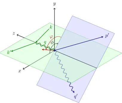
![Figure 7.4.: Beam spin sum/difference measured by the Hall A collaboration [62] (black circles) in proton-electron collisions](https://thumb-eu.123doks.com/thumbv2/1library_info/5555213.1689165/87.892.170.764.123.494/figure-difference-measured-collaboration-circles-proton-electron-collisions.webp)
![Figure 7.5.: Electron beam spin asymmetry A LU (φ) measured by the CLAS collaboration [64]](https://thumb-eu.123doks.com/thumbv2/1library_info/5555213.1689165/88.892.135.720.123.309/figure-electron-beam-spin-asymmetry-measured-clas-collaboration.webp)