47 Thomas Engl

(1)

D is se rt at io ns re ih e P hy si k - B an d 4 7

A Semiclassical Approach to Many-Body Interference in Fock-Space

Thomas Engl

47

9 783868 451283

ISBN 978-3-86845-128-3

Thomas Engl

ISBN 978-3-86845-128-3

theoretical methods. In this thesis, a non-perturbative semiclassical approach is developed, which allows to analytically study many-body interference effects both in bosonic and fermionic Fock space and is expected to be applicable to many research areas in physics ranging from Quantum Optics and Ultracold Atoms to Solid State Theory and maybe even High Energy Physics.

After the derivation of the semiclassical approximation, which is valid in the limit of large total number of particles, first applications manifesting the presence of many-body interference effects are shown. Some of them are confirmed numerically thus verifying the semiclassical predictions. Among these results are coherent back-/

forward-scattering in bosonic and fermionic Fock space as well as a many-body spin echo, to name only the two most important ones.

(2)

Thomas Engl

A Semiclassical Approach to Many-Body Interference in Fock-Space

(3)

Herausgegeben vom Präsidium des Alumnivereins der Physikalischen Fakultät:

Klaus Richter, Andreas Schäfer, Werner Wegscheider, Dieter Weiss

Dissertationsreihe der Fakultät für Physik der Universität Regensburg, Band 47

Dissertation zur Erlangung des Doktorgrades der Naturwissenschaften (Dr. rer. nat.) der naturwissenschaftlichen Fakultät II - Physik der Universität Regensburg vorgelegt von

Thomas Engl aus Roding im Juni 2015

Promotionsgesuch eingereicht am: 10.06.2014 Die Arbeit wurde angeleitet von: Prof. Dr. Klaus Richter

Prüfungsausschuss: Vorsitzender: Prof. Dr. Rupert Huber 1. Gutachter: Prof. Dr. Klaus Richter 2. Gutachter: Prof. Dr. Milena Grifoni weiterer Prüfer: Prof. Dr. Andreas Schäfer

(4)

Thomas Engl

A Semiclassical Approach to

Many-Body Interference

in Fock-Space

(5)

in der Deutschen Nationalbibliografie. Detailierte bibliografische Daten sind im Internet über http://dnb.ddb.de abrufbar.

1. Auflage 2015

Umschlagentwurf: Franz Stadler, Designcooperative Nittenau eG Layout: Thomas Engl

Druck: Docupoint, Magdeburg ISBN: 978-3-86845-128-3

Weitere Informationen zum Verlagsprogramm erhalten Sie unter:

www.univerlag-regensburg.de

(6)

A Semiclassical Approach to Many-Body Interference in

Fock-Space

DISSERTATION

ZUR ERLANGUNG DES DOKTORGRADES DER NATRUWISSENSCHAFTEN (DR. RER. NAT.)

DER FAKULT ÄT F ÜR PHYSIK DER UNIVERSIT ÄT REGENSBURG

vorgelegt von Thomas Engl

aus Roding

im Jahr 2015

(7)

Prüfungsausschuss: Vorsitzender: Prof. Dr. Rupert Huber 1. Gutachter: Prof. Dr. Klaus Richter 2. Gutachter: Prof. Dr. Milena Grifoni weiterer Prüfer: Prof. Dr. Andreas Schäfer

(8)

Dedicated to Martin C. Gutzwiller

(9)

(10)

4.3 The Semiclassical Propagator in Quadrature Representation 54 4.3.1 Propagator between quadratures with the same phase 54 4.3.2 Propagator between quadratures with different phases 56 4.3.3 An initial value representation using quandratures . 57 4.4 The Semiclassical Propagator in Fock State Representation 59 4.4.1 The propagator . . . 59

4.4.2 The (approximate) semi-group property . . . 62

5 Fermions 67 5.1 The Propagator using Klauder’s Coherent State Represen- tation . . . 68

5.1.1 The Path Integral . . . 68

5.1.2 Stationary phase approximation . . . 70

5.2 The Semiclassical Propagator in Fermionic Fock States . . . 72

5.2.1 The complex Path Integral for the Propagator in Fock state Representation . . . 72

5.2.2 Semiclassical Approximation . . . 76

IIIInterference Effects in Bosonic Fock Space 83 6 Non-Interacting Systems 85 6.1 The Transition Probability for Quadratures . . . 85 6.1.1 The exact propagator in quadrature representation . 85 6.1.2 Propagation between quadratures with the same phase 87 6.1.3 Propagation between quadratures with different phase 89

(12)

CONTENTS ix

6.2 The Transition Probability in Coherent States . . . 90

7 Many-Body Coherent Backscattering 95 7.1 Chaotic Regime . . . 95

7.1.1 Diagonal approximation . . . 96

7.1.2 Coherent backscattering contribution . . . 97

7.1.3 Loop contributions . . . 101

7.2 Weak Coupling Regime . . . 108

7.2.1 The propagator in quadrature representation for diagonal Hamiltonians . . . 109

7.2.2 Transition probability for weak hopping . . . 115

8 Many-Body Transport 119 8.1 Formulation of many-body transport . . . 119

8.2 Exact treatment of the leads . . . 121

8.3 Calculating Observables . . . 125

8.3.1 A semiclassical formula for expectation values of single- particle observables . . . 125

8.3.2 Diagonal approximation: Rederiving the Truncated Wigner Approximation . . . 128

8.3.3 Interference effects: Sieber-Richter Pairs and One- Leg-Loops . . . 129

9 The fidelity for interacting bosonic many-body systems 133 9.1 The Fidelity Amplitude . . . 133

9.1.1 Disordered system . . . 134

9.1.2 Short Time Behavior . . . 136

9.2 The Loschmidt echo . . . 137

9.2.1 Background contribution . . . 137

9.2.2 Incoherent contribution . . . 138

9.2.3 Coherent contribution . . . 140

9.3 Discussion and comparison with numerical data . . . 142

9.3.1 Fidelity . . . 142

9.3.2 Loschmidt echo . . . 145

IV Interference Effects in Fermionic Fock Space 151 10 The Transition Probability for Fermionic Systems 153 10.1 Diagonal approximation . . . 154

(13)

10.2 Coherent backscattering like contribution . . . 155

10.3 Discussion . . . 157

10.4 Further discrete symmetries . . . 159

11 Many-Body Spin Echo 163 11.1 The spin-echo setup . . . 163

11.2 Leading order contributions . . . 166

11.3 No spin-flips: Semigroup property . . . 170

11.4 Discussion of the results . . . 172

11.5 Concluding remarks . . . 173

11.5.1 Higher order contributions . . . 173

11.5.2 Incomplete spin flips . . . 178

12 Many-Body Spin Fidelity 181 12.1 Unitarity . . . 187

12.2 General Results . . . 188

12.2.1 Odd number of particles . . . 188

12.2.2 Even number of particles . . . 189

13 Summary & Outlook 191 13.1 Summary . . . 191

13.2 Outlook . . . 197

List of Publications 199 Acknowledgements 201 Appendix 205 A The Semiclassical Propagator for Bosons 205 A.1 The classical Hamiltonian for a Bose-Hubbard systems in quadrature representation . . . 205

A.2 The stationary phase approximation to the bosonic propagator in quadrature representation . . . 208

A.3 The basis change from Quadratures to Fock states for the semiclassical propagator . . . 211 B The Feynman Path Integral for Fermions using complex

variables 219

(14)

CONTENTS xi

C Semiclassical propagator for Fermions 229

C.1 Derivation of the semiclassical prefactor . . . 229

C.2 Simplification of the semiclassical prefactor . . . 238

D The bosonic transition probability in the weak coupling regime 241 D.1 Determination of the trajectory and its action . . . 241

D.2 Transformation to Fock states . . . 243

D.2.1 The coherent state propagator for weak hopping . . 245

D.2.2 The propagator for weak hopping in number representation . . . 247

E Derivation of the propagator for open systems 249 E.1 Splitting off the leads . . . 251

E.2 The full propagator . . . 253

E.3 Getting real actions and stationary phase approximation . . 255

F Loop contributions 259 F.1 Two-leg-loops . . . 260

F.1.1 Phase-space geometry . . . 260

F.1.2 Partner trajectory . . . 263

F.1.3 Existence . . . 263

F.1.4 Action difference . . . 264

F.1.5 Density of encounters . . . 266

F.2 One-leg-loops . . . 268 G Hubbard-Stratonovich transformation 271

Bibliography 275

(15)

(16)

CHAPTER 1 Introduction

1.1 Classical Mechanics gone Quantum

1.1.1 The first quantum revolution

100 years ago, not only the first world war broke out, but also James Franck and Gustav Hertz showed in their experiment that the electrons in an atom can have only certain quantized energies [1]. The Franck-Hertz experiment was the first experimental proof of the quantum nature of atoms, and also resulted in a Nobel prize for Franck and Hertz in 1925. At that time, Bohr’s heuristic atom model [2], which in a way could be considered as the first semiclassical model since it used quantized but otherwise classical orbits, was considered to be the correct theory to describe the inner structure of atoms.

The Bohr-Sommerfeld quantization rule actually yielded the correct energy levels for the hydrogen atom even including fine structure. However, although many physicists – among them Bohr, Born, Kramers, Land´e , Sommerfeld and van Vleck – tried to compute it, the correct ground state energy of Helium could not be reproduced [3].

This failure to compute the energy levels of Helium marked the end of the “old quantum theory”. Finally, in 1925, works by Louis de Broglie, Werner Heisenberg and Erwin Schr¨odinger culminated in the Schr¨odinger equation [4]. A test of the thus developed “new quantum theory” is the scattering of electrons on a Nickel cristal [5], which shows the same diffrac- 1

(17)

tion pattern as the scattering of X-rays on Nickel cristals – by the way a Nobel prize in 1914 for Max von Laue.

After the establishment of the new quantum theory, it became clear that the Bohr-Sommerfeld quantization rule follows from the semiclassical WKB or EBK approximation [6], respectively, such that denoting Bohr’s atom model as a semiclassical description can actually be justified. How- ever, WKB and EBK quantization is valid for classically integrable systems only, thus explaining the failure of the old quantum theory for He- lium, which is a chaotic three-body system. On the other hand, within the new quantum theory, the WKB approximation was the first connection of a quantum object, namely the wave function, with classical trajectories and their actions. Such a connection was also established in 1928 by van Vleck, who made use of probabilistic arguments, in order to approximate the quantum mechanical propagator in configuration space in terms of classical trajectories starting and ending at the initial and final position, respectively, and their actions [7]. It is worth to notice that van Vleck’s result coincides for short times with Pauli’s short time approximation [8].

In 1948, Richard Feynman established another connection between the quantum mechanical propagator in configuration space and paths connecting the initial and final position [9]. However, in his path integral formal- ism, it is not just the classical trajectories, one has to sum over, but over all – classical and non-classical – paths, which ensures that also tunneling effects are included. The latter is important to notice, since classical trajectories do not tunnel, and therefore tunneling effects can not be resembled by semiclassical descriptions based on classical trajectories, unless they are incorporated artificially [10]. It was then Martin C. Gutzwiller [11], who unfortunatelly died one year ago, who applied a stationary phase approximation [12–14] to Feynman’s path integral, in order to show that van Veck’s result has to be modified by phases typically denoted as Maslov indexes, given by the number of focal points of the trajectory [6]. This propagator is nowadays referred to as van-Vleck-Gutzwiller propagator. The linearity and the consequential interference of the quantum theory is thereby resembled by the fact that the van-Vleck-Gutzwiller propagator is computed fromall classical trajectories joining the initial and the final position.

In the very same publication [11], Gutzwiller also showed, how to per- form the Laplace transfromation of the van-Vleck-Gutzwiller propagator from time to energy domain in order to arive at a semiclassical Green’s function, which is then no longer given by classical trajectories with fixed time, but with fixed energy. From the Green’s function, also the density of states of a quantum system can be computed [15], and Gutzwiller’s approx-

(18)

1.1. CLASSICAL MECHANICS GONE QUANTUM 3

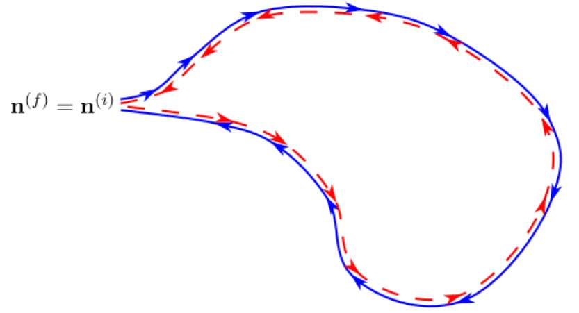
(a) Diagonal pair (b) Sieber-Richter pair

Figure 1.1: (a) A diagonal and (b) Sieber-Richter pair as those appearing in the computation of the spectral form factor.

imation provides a way to also connect this quantum mechanical quantity to classical trajectories. In fact, it was again Gutzwiller [16], who showed that semiclassically, the density of states can be decomposed into a smooth (Weyl) part [17] and an oscillatory part, where the latter is given by a sum over periodic orbits. This is Gutzwiller’s famous trace formula, which is valid for classically chaotic systems like – guess what – the Helium atom.

In addition, latest with Berry’s diagonal approximation [18], it became evident that semiclassics is a very powerful tool for studying universal quantum effects in single-particle systems. Among these effects are weak localization [19–21], weak anti-localization [22, 23], coherent backscattering [24], the decay of the Loschmidt Echo [25, 26] and the spectral form factor [18].

On the other hand, however, based on Bohiga’s, Giannoni’s and Schmidt’s conjecture that systems with chaotic classical counterpart behave as if their hamiltonian would be a random matrix [27], many random matrix theory (RMT) results showed that the results obtained in diagonal approximation were often only leading order effects. It then took until the beginning of the new millenium to identify the next to leading order contributions for two dimensional systems [28], which are now often denoted as Sieber-Richter pairs (see Fig. 1.1(b) for a sketch of these pairs) or – more generally – loop contributions. Within their approach, Martin Sieber and Klaus Richter were also able to solve the problem of the missing normalization of the transmission probabilities for open chaotic systems, which appears, when sticking to the diagonal approximation [21].

The semiclassical approach has then been extended not only to include higher order contributions, but also higher dimensions [29–38], and has now for the spectral form factor been shown to be able to reproduce the full RMT result [39]. Again, the corrections to leading order results in single-particle systems have been studied extensively using this approach.

For instance, the conductance of a chaotic conductor has been calculated to all orders in the inverse number of channels [34], as has been the density of states of Andreev Billiards [40, 41]. Within this approach, universal conductance fluctuations [20, 42–44] could also be described. Moreover, it

(19)

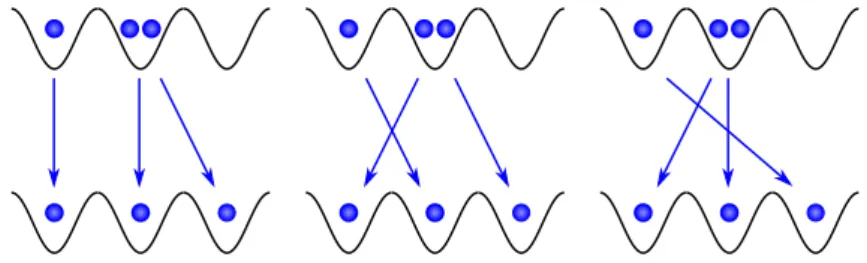
Figure 1.2: Three indistinguishable scattering processes, that give rise to many-body interference.

has been applied to the Loschmidt echo [45, 46], the conductance and ther- mopower of Andreev Billiards [47–49], transport of Bose-Einstein conden- sates through chaotic conductors [50], transport moments of chaotic conductors and Andreev Billiards [51–54]. Right now, even quantum graphs, which have eigenvalues given by the zeros of Riemann’s Zeta Functions, are under investigation [55]. Furthermore, this semiclassical approach to quantum chaotic transport can reproduce Anderson localization [56–58].

This already pretty long, but surely not complete list of applications, shows that semiclassics is very successful in describing universal quantum effects of single-particle systems. However, the methods to describe universal quantum effects are not (or only with a huge effort) able to describe many-body effects, if the total number of particles is large [59]. This is due to the additional many-body interference depicted in Fig. 1.2 due to the in- distuingishability of the particles and the necessary (anti-) symmetrization associated with it.

1.1.2 Second quantization

Indistinguishability, and the fact that the symmetrization or antisym- metrization of wave functions becomes intractable for large particle number was the reason for the development of second quantization [60]. There, every operator is written as a combination of so called creation and annihilation operators, with coefficients which are determined by the corresponding single-particle system, only. For the creation and annihilation operators there are two possible interpretations. Either they create and annihilate, respectively, a particle in a certain single-particle state, or a certain excitation of the ground state. The first interpretation is commonly used in quantum field theories [61], while the second one is used for example for the description of the quantum harmonic oscillator [62]. Actually, these two

(20)

1.1. CLASSICAL MECHANICS GONE QUANTUM 5

interpretations are equivalent, since any excitation can be interpreted as a quasi-particle [63]. When choosing the single-particle states in which the creation and annihilation operators create or annihilate particles or excita- tions as position states, the creation and annihilation operators are often denoted as field operators [64].

To the author’s knowledge, the use of semiclassical methods in Fock space is rather limited. For Bosons, these approaches are mainly based on coherent states [65–69], initial value representations in terms of the Herman-Kluk propagator [70, 71] or WKB and EBK approximations [72–

75]. While the latter is restricted to integrable systems, only, the first two approaches can be applied to any system, no matter whether it is integrable or not. If one wants to transfer the accomplishments in semiclassical methods for single-particle to many-body systems, they yield severe problems, though.

While an initial value representation may be very advantageous for numerical studies and integrable systems [71], it is not able to predict universal features analytically, since especially the loop contributions are not explicit in this case.

The coherent state propagator requires complex trajectories [65–69]

with complex action. Therefore, unlike the usual van-Vleck-Gutzwiller propagator [11], for each trajectory the action not only contributes a phase, but also a real exponential factor, which makes the usual argumentation of strongly oscillating terms due to action differences of not correlated pairs of trajectories impossible. However, this kind of reasoning is necessary in order to be able to restrict the analysis to diagonal [18] and loop contributions [21, 28–37]. It is worth to notice that “it may happen that the complex trajectory is close enough to a real one [...]” (cf.[76]), such that one can use a real trajectory, in order to approximate the contribution of a complex one [67, 76, 77], “[...] if the latter is not too deep into the complex plane.” (cf.[67]). However, as these statements already indicate, it is highly questionable, whether this approximation can be generally applied systematically, and the proponents of this approximation themselves recognized that it may give wrong or insufficient results [67, 76].

For fermions, the situation seems to be far worse. To the author’s knowledge, rigorous semiclassical approaches in Fock space are so far restricted to spin-chains [65, 69], which describe essentially distinguishable particles, since each particle is fixed to one position. For systems with spin- orbit interactions, kind of hybrid systems have been introduced, where the orbital degrees of freedom are treated in configuration space, while for the spins coherent states are used [23, 78–84].

(21)

(a) (b)

Figure 1.3: Classical (a) vs. quantum (b) discrete time random walk:

While in the classical random walk, the particle goes either to the left or to the right at each step, in the quantum random walk the wave function splits up at each step and interferes.

The problem with a semiclassical approach in Fock space is that due to the antisymmetry of the fermions, coherent states are described by anti- commuting Grassmann variables [61, 64] and therefore a stationary phase approximation to the straight forward coherent state path integral for instance yields as classical limit Grassmann valued equations of motions and actions. This is probably the reason, why the theories closest to a semiclassical one in fermionic fock space are up to now quaiclassical approaches, where a heuristic classical Hamiltonian is imposed [85, 86].

The aim of this thesis is to address and – if possible – lift these issues of semiclassical approaches in Fock space for both, Bosons and Fermions.

Once such semiclassical approaches are successfully derived, one may start to dream a little bit in which research areas they may be applied.

1.2 The Connection to Various Research Fields

1.2.1 Quantum Optics

To start with non-interacting systems, one possible field of application could be quantum walks [87–91], which became of special importance in the context of quantum computation [92] and quantum search algorithms [93].

While “In classical random walks, a particle starting from an initial site on a lattice randomly choses a direction and then moves to a neighboring site accordingly” (cf. [91]), in a quantum random walk, the wave function of a

(22)

1.2. THE CONNECTION TO VARIOUS RESEARCH FIELDS 7

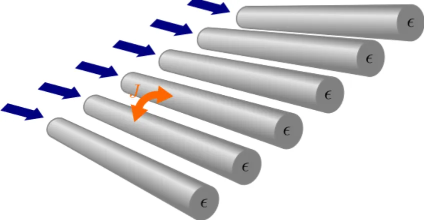
J

Figure 1.4: Schematic picture of seven ultra-cold atoms in an optical lattice consisting of five magneto-optical traps. The atoms can tunnel from one trap to a neighbouring one with a probability given by the hopping amplitudeJ.

particle splits at each site into two components, which finally will interfere again [94]. Such quantum walks are mainly performed using photons.

Quantum walks based on photons are usually classified as follows: In discrete time quantum walks, beam splitters are used, such that for discrete time steps, a photon can enter one of two wave guides [90, 95–97]. It is worth to mention the easiest case of a discrete time quantum walk having just one beam splitter, namely the well known Hong-Ou-Mandel effect [98].

In continuous time quantum walks, on the other hand, several waveguides are arranged periodically close to each other, such that a photon can tunnel from one wave guide to the other one [91, 99–101]. In both cases, time can due to the fixed speed of photons (namely the speed of light), be mapped to the position of the photon along a certain direction [102], which is often chosen to be thez-direction.

Interestingly, even disorder can be realized in these systems. For beam splitter this is by implying so called coin operators, which – classically speaking – change the probability to go to either side [97], while for waveguide arrays the refractive index can be adjusted for each wave guide sepa- rately [91]. The fact that, for waveguide arrays the system can be changed by changing the waveguides only, also allows for instance to study nonlinear effects [102, 103].

Since these experiments are usually done with one single [91, 95, 97, 99, 102, 103] or two photons [96, 100], these experiments can not be described using classical electrodynamics. However an approach based on a Hamilto- nian given in terms of creation and annihilation operators as the one which will be considered in this thesis may be applied.

Finally, quantum walks are not only possible by using photons, but also with ultra-cold atoms and ions [104–108].

(23)

1.2.2 Ultra-cold Atoms in Optical Lattices

These systems consist of several atoms, which are at very low tem- peratures (usually a few nK) trapped in a periodic potential built up by interfering laser beams, which are adjusted such that they form standing waves [109] and are generally described by Hubbard models [110]. An optical lattice consisting of five magneto-optical traps, which are often also denoted as sites, and seven particles is schematically shown in Fig. 1.4.

An advantage of these systems is their vast controllability [111]. By using Feshbach resonances [112–115] for instance, the scattering length, which in turn determines the interaction strength, can be adjusted and tuned within a wide range [116, 117].

Additionally, by increasing the intensities of the used laser beams, the tunneling probability,i.e. the probability for an atom to tunnel from one well of the optical lattice to another one, can be decreased, resulting in a relative increase of the interactions compared to the kinetic energy, which is often denoted as hopping amplitude. If the tunneling probability is in- creased so far that the hopping amplitude is much smaller than the interaction strength, the energy is dominated by the latter and tunneling from one well to an other is energetically suppressed or even forbidden. This regime is called the Mott insulating phase [118, 119] and for ultra-cold atoms it is accessible by the prescribed procedure. In fact, when increasing the laser intensity, bosonic ultra-cold atoms undergo a quantum phase transition from a superfluid to a Mott insulating phase [120, 121].

For Fermions the Mott insulating phase also appears when the hopping amplitude is not negligible but much smaller than the interaction strength for half filling and a phase transition from Mott insulating to superconduct- ing can be achieved by hole doping, i.e. by removing particles [122–124].

For fermions, the Mott insulating ground state is also predicted to be an- tiferromagnetic [123].

The Mott insulating phase also allows a simple scheme for loading an optical lattice with atoms [125–127]. In the same way, it can be used, for fixing the atoms after time evolution and determine the number of atoms in each well by high resolution imaging techniques [128, 129].

Finally, the energy of each well of the periodic potential can also be adjusted individually, thus giving the possibility to create optical disorder [130] and, despite the fact that atoms have no electrical charge (therefore a magnetic field does not have any effect on their motion) time reversal invariance can be broken by artificial [131–134] and synthetic gauge fields [135].

(24)

1.2. THE CONNECTION TO VARIOUS RESEARCH FIELDS 9

These properties and especially the high controllability of the systems suggest that ultra-cold atoms can be used as simulators for condensed matter systems [111, 125] like for example graphene [136]. Since recently also spin-orbit interaction have been realized with ultra-cold atoms [137–139], one could also think of simulating spintronics in optical lattices.

1.2.3 Spintronics

Spintronics is essentially the investigation of spin related effects, mainly solid state systems, and aims towards a spin-based, rather than the con- ventionally charge-based, information transport [140–142]. The punchlines there, are e.g. the generation of spin polarization, injection of spin polarized currents as well as possibilities to manipulate and measure them. Very often hetero-structures composed of ferromagnetic materials and semicon- ductors or ferromagnetic and insulating materials are used. In these systems, the ferromagnets serve as injectors or detectors of spin polarization.

Very prominent effects in such hetero-structures are giant magnetoresistance (GMR) [143, 144] and tunneling magnetoresistance (TMR) [145].

For both, GMR and TMR, the (electrical) resistance is much larger if the magnetizations of the two ferromagnetic layers have opposite directions than if they are parallel. The difference in the setup between them is that for GMR a semiconductor is placed between two ferromagnets, while for TMR a so called magnetic tunnel junction is used, where an insulator (=tunneling barrier) is sandwiched by two ferromagnets. These two effects also made successfully their way to industrial applications and have been established in read heads in hard disk drives.

Another effect, which seems to be on its way to industrial applications in so called racetrack memory [142] are spin transfer torque effects [146].

In these effects, spin-polarized particles crossing a domain wall in a ferromagnetic material transfers its magnetic moment to the substrate and thus moves the domain wall.

Relativistic effects like Bychkov-Rashba [147] and Dresselhaus spin- orbit interactions [148] are also important in spintronics. For instance, they are the key elements of spin-hall [149, 150], quantum spin hall [151–

154] and spin-based transistors [155]. While spin hall and quantum spin hall effect are both based on the fact that due to intrinsic spin-orbit interaction particles with spin up and spin down, respectively, moving in the same direction are dragged to opposite directions perpendicular to the overall direction of the current, in the spin field effect transistor [155] the

(25)

spin orbit interaction strength is determined by an external gate voltage.

The spin-orbit coupling then leads to spin-precession of the crossing particle. The source and drain are magnetized, such that the electrons entering are also spin-polarized and can enter the drain only if the spin-precession is such that their spins are parallel to the magnetization in the drain.

So far, spintronics mainly focuses on single-particle effects [140–142, 156], for which using a Fock space approach of indistinguishable particles is not quite reasonable. However, for studying many-body effects in spintronics devices, the techniques developed in this thesis might be of particular help.

1.2.4 Many-Body effects in condensed matter physics

More generally, it is important to study many-body effects in condensed matter systems. Well known amongst these are for instance the Coulomb blockade [157–163], inelastic and elastic co-tunneling [164–168] and the Kondo effect [168–170]. The Coulomb blockade arises due to the Coulomb repulsion of the electrons in a quantum dot coupled to leads via tunnel junctions. This repulsion implies a large energy cost in order to add a further electron which in turn results in peaks of the current-voltage char- acteristic only for specific voltages corresponding to the energy needed in order to add a electron to the quantum dot.

In quantum dots, cotunneling, where two electrons – one into the quantum dot and one out of the quantum dot – tunnel at the same time, and the Kondo effect are corrections to the Coulomb blockade at low temper- atures. The Kondo effect originally refers to a minimum of the resistance as a function of temperature in a metal [170] due to scattering off magnetic impurities, where the impurity and the electron exchange their spin.

Nowadays, the Kondo effect is mainly studied in quantum dots and carbon nanotubes [168, 171–188] and became a test case for many-body theories in condensed matter physics [189–196].

Due to their similarities, quantum dots are also regarded as artificial (two dimensional) atoms [177, 197, 198] and even the formation of artificial molecules [199–201] is possible using quantum dots.

(26)

1.3. OUTLINE OF THIS THESIS 11

1.2.5 Chemical Physics

Real Atoms and Molecules, on the other hand, are the central objects in chemistry. In fact, the chemical physics community has made extensive use of semiclassical methods and played an important role in their development [70, 202–209].

Starting with Ref. [209] Miller and coworkers started the study of molecular collisions, which give rise to electronic transitions within the molecules and succeeded to describe resonance effects [210]. There, the electronic degrees of freedom have been treated semiclassically, while the nuclear motion was incorporated classically [209]. After that, in order to be able to derive electronic and nuclear motion on the same footing, they turned to deriving a classical theory of these collisions [85, 211–213]. These classical approaches are basically determined by a mapping of angular momenta, including spin, to classical action angle varibles [202, 214].

Motivated by this process, Miller and White tackled the problem of deriving a classical Hamiltonian for a second quantized fermionic Hamilonian already in 1986 [86]. By using similar techniques they managed to derive a Schwinger representation of the angular momentum [215]. Later on, it has been used heuristically in a semiclassical initial value representation including Langer substitutions [216].

The thus developed techniques have also been applied to electronic transport through a single quantum dot [217], two coupled quantum dots [218] and molecular junctions [219].

The problem with the Meyer-Miller-Stock-Thoss approach developed in [85, 86, 215, 216] is, however, that the Fock states, i.e. those states with well defined occupations of the single-particle states, are fixed points of the classical motion [220]. Moreover, it is based on heuristic mapping approaches, instead of a rigorous derivation by means of a path integral, where the classical Hamiltonian appears naturally. Finally, it does not yield any insight, what the effective Planck constant ¯h_eff, i.e. the small parameter in a stationary phase analysis of the path integral, actually is.

1.3 Outline of this thesis

During this thesis, an answer to this last question, what the effective Planck constant is, will be also given. This will be accomplished by first deriving an exact path integral both for Bosons and Fermions based on

(27)

complex variables, which will also determine the classical limit of the second quantized theory.

Before that, however, a brief introduction to the basic concepts used during this thesis will be given in the first part. This introduction contains a short review of the derivation of the path integral and the van-Vleck- Gutzwiller propagator in configuration space in Chapter 2, the basic concepts of second quantization as well as important states in Fock space and their properties in Chapter 3 for both, Bosons and Fermions.

The second part, finally, is dedicated to the construction of path integrals and semiclassical approximations for the propagator in Fock space based on complex variables for Bosons in Chapter 4 as well as for Fermions in Chapter 5. For the bosonic proapgator, it is also shown that the semiclassical approximation fulfills the semi-group property.

The thus derived bosonic propagator is applied in Part III to bosonic many-body systems, starting with non-interacting systems like quantum walks in photonic wave guide arrays in Chapter 6, and then turning to describing coherent backscattering in Fock space for interacting particles in Chapter 7, many-body transport of interacting Bosons in Chapter 8 and finally to the fidelity decay for interacting ultra-cold atoms in Chapter 9.

Similarly, in the fourth part of this thesis, fermionic many-body interference effects are considered by applying the approach derived in Chapter 5.

These interference effects are enhanced and vanishing transition probabilities between Fock states, which are investigated in Chapter 10, as well as a many-body spin echo resulting from an intermediate manipulation of spins in Chapter 11 and a related quantity, which is here denoted as spin fidelity in Chapter 12.

Finally, concluding remarks as well as future perspectives are given in Chapter 13.

(28)

Part I

Basic concepts

13

(29)

(30)

CHAPTER 2 Semiclassics for Single-Particle Systems

2.1 The Path Integral Representation of the Propagator

2.1.1 The quantum mechanical propagator

Semiclassics as it is understood through out this thesis, is based on a stationary phase approximation to the quantum mechanical propagator (or time evolution operator), which is defined as the operator which connects the state |ψ(ti)i at initial time ti with the one at final time tf,|ψ(tf)i by [221]

|ψ(tf)i= ˆK(tf, ti)|ψ(ti)i. (2.1) Since in quantum mechanics|ψ(t)isatisfies the time dependent Schr¨odinger equation

i¯h∂

∂t|ψ(t)i= ˆH(t)|ψ(t)i,

the propagator is the solution to the operator differential equation [13, 62]

i¯h∂

∂t

Kˆ(t, t_i) = ˆH(t) ˆK(t, t_i), (2.2) with initial condition

K(tˆ _f =t_i, t_i) = ˆ1, (2.3) 15

(31)

where ˆH(t) is the (time-dependent) quantum mechanical Hamilton operator (or in short, quantum Hamiltonian), ˆ1 is the unity operator, t is the time, i is the imaginary unit and ¯h is Planck’s constant.

Formally, the solution of eqns. (2.2,2.3) can be written as [62, 221]

K(tˆ f, ti) = ˆT exp





−i

¯ h

tf

Z

ti

dtH(t)ˆ





, (2.4)

where ˆT is the time ordering operator, which sorts the factors of the product right to it such that their time arguments decrease from left to right,e.g.for a product of two operators ˆA₁(t) and A₂(t) [13, 62],

TˆAˆ₁(t₁) ˆA₂(t₂) =

(Aˆ₁(t₁) Â₂(t₂) ift₁≥t₂, Aˆ₂(t₂) Â₁(t₁) ift₂> t₁. More generally, fornoperators Â1(t), . . . ,Aˆn(t),

Tˆ

n

Y

j=1

Aˆj(tj) = X

σ∈Sn





n−1

Y

j=1

Θ t_σ(j)−t_σ(j+1)





n

Y

j=1

Aˆ_σ(j)(t_σ(j)), (2.5)

where the product Q

j is defined such that j increases from left to write, and Sn is the symmetric group of n, i.e. the group of all n-permutations, and

Θ(x) =

(1 ifx≥0, 0 ifx <0.

is the Heaviside step function. A product of the form (2.5) is often also denoted as time-ordered product.

The combination ˆT exp (. . .), as it appears in (2.4) and is usually called time-ordered exponential, should be evaluated by first expanding the exponential using its Taylor series and after that applying the time ordering operator to each summand individually. Note that, although

hH(t),ˆ H(t)ˆ i

−= 0,

the Hamiltonian at timetdoes in general not commute with the Hamilto- nian at timet⁰,

hH(t),ˆ H(tˆ ⁰) i

−6= 0.

(32)

2.1. THE PATH INTEGRAL FOR THE PROPAGATOR 17

Hereh A,ˆ Bˆi

− denotes the commutator of the operators ˆAand ˆB.

In order to further evaluate the propagator, one has to choose a certain basis. In principle, one could choose any basis, however since this part is meant for illustration of the basic methods used later on only the configuration space basis, given by the position eigenstates|riis used here.

Inserting a unit operator in terms of position eigenstates [221, 222], ˆ1 =

Z

d^Dr|ri hr|, (2.6) whereDis the spatial dimensionality of the systemm, in (2.1) and project- ing it to the position eigenstate|ri yields for the evolved wavefunction in configuration space [223]

ψ(r, t_f) = Z

d^Dr⁰K r, t_f;r⁰, ti

ψ r⁰, ti

,

whereψ(r, t) =hr|ψ(t)i and K r, t_f;r⁰, ti

= D

r

Kˆ (t_f, ti) r⁰

E

(2.7) is the propagator in configuration space representation. The modulus square of this complex quantity then yields the probability that if a particle is at timeti at position r⁰, it is found at time tf at position r. Therefore, by choosing the initial state to be a Dirac delta in configuration space, ψ(r⁰, t_i) =δ(r⁰−r), due to the normalization of the wave function,

Z d^Dr⁰

K r⁰, t_f;r, t_i

2 = 1.

Moreover, the initial condition of the propagator (2.3) reads in configuration space

K r⁰, t;r, t

=δ r⁰−r .

Finally, the time evolution operator has to be unitary and satisfy [13]

K(tˆ f, t) ˆK(t, ti) = ˆK(tf, ti)

for any timet,i.e.propagating a state twice in time has to result in the same wave function as propagating it once over the whole duration. Moreover, it has to be unitary [13]. Thus, the propagator in configuration space has

(33)

to satisfy the semi-group properties Z

d^Dr⁰⁰K r⁰, t_f;r⁰⁰, t

K r⁰⁰, t;r, t_i

=K r⁰, t_f;r, t_i

, (2.8a)

Z

d^Dr⁰⁰K^∗ r⁰⁰, t_f;r⁰, t

K r⁰⁰, t;r, ti

=K r⁰, t_f;r, t_f

, (2.8b)

for any arbitrary timet.

2.1.2 The Path integral

Despite all these nice properties, one still has to evaluate the time ordered product, in order to find the propagator in configuration space representation, a very difficult problem without general solution. However, Feynman found a way out of this problem by his famous path integral approach [9]. Here we follow mainly Refs. [12, 13].

First, Trotter’s formula [224] is used, in order to split the time ordered exponential into an (infinite) product of exponentials with (infinitesimaly) small time steps [12, 13],

Tˆexp





 i

¯ h

tf

Z

ti

dtH(t)ˆ





= lim

M→∞

M

Y

m=1

exp

−iτ

¯

hH(tˆ _f −mτ)

, (2.9)

where τ = (t_f −t_i)/M. Recall that the product is defined such that the value ofm increases from left to right.

Using (2.9) in (2.7), inserting a unit operator in position representation (2.6) between ever two exponentials and finally a unit operator in momentum representation [222],

ˆ1 = Z

d^Dp|pi hp|,

left to every exponential, yields the path integral representation of the propagator in position space,

K r, t_f;r⁰, t_i

= lim

M→∞

Z d^Dp₀

Z d^Dr₁

Z

d^Dp₁. . . Z

d^Dr_M Z

d^Dp_M

M

Y

m=0

hr_m+1|p_mi

p_m

exp

−iτ

¯ h

Hˆ(t_i+mτ)

r_m

,

(34)

2.1. THE PATH INTEGRAL FOR THE PROPAGATOR 19

wherer0 =r⁰ and rM+1 =r. The matrix elements can then be evaluated by making use of the fact that the quantum Hamiltonian has the form

Hˆ = 1

2µpˆ²+V(ˆr),

where µ is the mass of the particle, V(r) the potential and ˆp and ˆr the momentum and position operator, respectively. Using the Baker-Campbell- Hausdorff formula [13], in the limitM → ∞, each exponential can be split into two exponentials, where the first one consists of the momentum and the second one depends on the position operator, only. Note that this does not apply in the presence of magnetic field, however one can show that the final form of the path integral is the same up to replacing the momentum pbyp−^q_cA(r) withq,candA being the charge of the particle, the speed of light and the vector potential, respectively [12]. Then, one can let act every momentum operator to the left and every position operator to the right, finally yielding [12, 13]

K r, tf;r⁰, ti

=

Mlim→∞

Z d^Dp₀ (2π¯h)^D

Z d^Dr1

Z d^Dp₁ (2π¯h)^D . . .

Z d^DrM

Z d^Dp_M (2π¯h)^D exp

(i

¯ h

M

X

m=0

[p_m·(r_m+1−r_m)−τ H(p_m,r_m;t_i+mτ)]

) ,

(2.10)

with the classical Hamiltonian resulting from the quantum one by replacing the momenum and position operator by real numbers, which are the momentum and position, respectively,

H(p,r) = p²

2µ+V (r). (2.11)

Eq. (2.10) is often written in the short-hand notation [13]

K r, tf;r⁰, ti

=

r

Z

r⁰

D[p(t),r(t)] exp i

¯

hR[p(t),r(t)]

,

where the limits of the integral indicate that the initial and final positions are fixed tor⁰ and r, respectively and

R[p(t),r(t)] =

tf

Z

ti

dt[p·r˙−H(p(t),r(t);t)]

(35)

is the action of the path (p(t),r(t)).

The name “path integral” comes from the fact that the integral Z

D[p(t),r(t)]. . .

runs over all paths in phase space. These paths, which are schematically depicted in Fig. 2.1(a), are neither restricted to the (classically) allowed regions nor do they need to be smooth.

Finally, making use of the form (2.11) of the classical Hamiltonian the integrals over the intermediate momenta can be carried out [12, 13],

K r, t_f;r⁰, t_i

=

Mlim→∞

Z

d^Dr₁. . . Z

d^Dr_M exp

iτ

¯ h

M

P

m=0

hµ

2τ (rm+1−rm)²−τ V(rm) i

(2πi¯hτ /µ)

D(M+1) 2

, (2.12) which finally connects the propagator with the Lagrange function of the system by [13, 94]

K r, tf;r⁰, ti

=

r

Z

r⁰

D[r(t)] exp i

¯

hR[ ˙r(t),r(t)]

, (2.13)

with the action of the path ( ˙r(t),r(t))

R[ ˙r(t),r(t)] =

tf

Z

ti

dtL( ˙r(t),r(t);t) =

tf

Z

ti

dt µ

2r˙²(t)−V(r(t))

.

It is important to notice that the path integral runs over paths that are not necessarily restricted to the classically allowed region.

The huge advantage of the path integral representation is that one clearly sees the origin of interference: There are essentially an infinite number of possible paths a particle can take. However, during its evolution it will pick up a phase, which is given by the action of this path, and therefore every path yields a different phase. Finally, all paths add up and therefore interference occurs.

(36)

2.2. THE SEMICLASSICAL APPROXIMATION 21

(a) Possible paths summed over in the path integral

(b) Classical paths among the quantum ones shown in (a) se- lected by the stationarity condition

Figure 2.1: Selection of classical paths due to the stationary phase condition. The shaded areas mark classically forbidden regions. While the quantum paths can be non-smooth and cross these regions the classical ones can not

2.2 The Semiclassical Approximation

The path integral (2.12) is also the starting point for the semiclassical approximation to the propagator. It is based on the observation that in many relevant cases, the actions are much largher than ¯h. Then the integrals in (2.12) can be evaluated using the stationary phase approximation [11].

2.2.1 Stationary phase approximation

The stationary phase approximation is a method to evaluate integrals of the form

I =

∞

Z

−∞

dxg(x) exp [iλf(x)],

whereλ1 is a large parameter andg(x) a smooth function. As illustrated for the case of the integral representation for the Bessel function in Fig. 2.2, the integrand oscillates very fast as a function ofx except for those values ofx close to the stationary pointsx₁, . . . , x_n off, for which

∂

∂xf(x) x=xj

= 0. (2.14)

Therefore, one first splits the integral into n integrals, where the j-th integral runs over an interval containing the j-th stationary point and the

(37)

-1 -0.5 0 0.5 1

0 0.2 0.4 0.6 0.8 1

τ

(a) Comparison between the exact (red) integrand and the one in the stationary phase approximation (blue) for the integral representation of the fifth Bessel function at x= 65.

-60 -40 -20 0 20

0 0.2 0.4 0.6 0.8 1

τ

(b) Argument of the integrand for the integral representation of the fifth Bessel function atx= 65.

Figure 2.2: The integrand of the integral-representation of then-th Bessel function, Jn(x) = Rπ

0 τcos [nτ π−xsin (τ π)], strongly oscillates except in the region around x ≈ 0.47549 ((a), where the argument of the cosine is stationary (b). Therefore, the main contribution to the integral stems from this region.

exponential is expanded up to second order around the stationary point.

Dropping the higher order contributions off(x) yields an error of the order of 1/λ[12]. Since the main contributions toIstem from regions close to the stationary points – more precisely from the interval [x−1/√

λ, x+ 1/√ λ]

[12] – each integral can be extended to the whole real axes,

I ≈

n

X

j=1

∞

Z

−∞

dxg(x+xj) exp i

¯ h

f(xj) +1

2f⁰⁰(xj)x²

,

withf⁰⁰ denoting the second derivative of f. Fig. 2.2(a) shows for the case of the Bessel function how this approximation indeed resembles the exact integral, within the region where it varies slowly, very well. Expanding g(x−x_j) around zero then allows to compute the integrals term by term, where the contributions from the x-dependent terms of g again lead to contributions of the order 1/λ, whereas the leading order contribution is of the order of 1/√

λ [12]. Thus, finally I is within the stationary phase

(38)

approximation given by [12, 13]

I ≈

n

X

j=1

g(xj) s

2πi

λf⁰⁰(xj)exp [iλf(xj)]

=

n

X

j=1

g(xj) s

2π

λ|f⁰⁰(xj)|exp h

iλf(xj) + iπ

4sign f⁰⁰(xj)i .

(2.15)

with an error of the order 1/λ.

For higher dimensional system, the same steps can be performed and yields for scalar functionsg(x) and f(x) [14]

Z

d^Dxg(x) exp [iλf(x)]≈

n

X

j=1

g(xj)

s (2πi)^D

λ^Ddet^∂_∂x²^f2(xj)exp [iλf(xj)]

=

n

X

j=1

g(x_j) v u u t

(2π)^D λ^D

det^∂_∂x²^f2(x_j)

exph

iλf(x_j) + iβ(x_j)π 4 i

=

n

X

j=1

g(xj) v u u t

(2πi)^D λ^D

det^∂_∂x²^f2(xj)

exp h

iλf(xj)−iν(xj)π 2 i

, (2.16) where

β(x) =D−2ν(x),

and ν(xj) is the number of negative eigenvalues of the matrix of second derivatives off. Thus,β(x) is the difference in the number of positive and negative eigenvalues of∂²f /∂x².

Note that since in semiclassics this approximation is used frequently, it is also called the semiclassical approximation. Moreover, since the stationary phase approximation requires a large parameter in the phase, which is in semiclassics usually 1/¯h, the inverse of the large parameter, i.e. in this section 1/λ is called the effective Planck’s constant ¯h_eff

2.2.2 The van-Vleck-Gutzwiller Propagator

It was Martin C. Gutzwiller [11], who first applied the stationary phase approximation (2.16) to Feynman’s path integral (2.12). In terms of func- tional derivatives the stationarity condition (2.14) for the propagator reads

(39)

δ

δr(t)R[ ˙r(t),r(t)] = d dt

∂L

∂r(t)˙ − ∂L

∂r(t) = 0, (2.17) still with fixed boundary conditions r(ti) = r⁰ and r(t_f) = r. Eq. (2.17) is exactly Hamilton’s principle of the least action and leads to the Euler- Lagrange equations. Thus, the stationary phase approximation selects from all paths only the classical trajectories starting at intitial positionr⁰ and ending at the final oner(see Fig. 2.1 for a schematic example). Note that, in general, there might be several classical trajectories joining the two end points and thus following Eqns. (2.15,2.16) the semiclassical propagator will be a sum over classical trajectories, rather than just one term.

The semiclassical propagator in configuration space has thus the form K^(sc) r, t_f;r⁰, ti

= X

γ:r⁰→r

Aγ r, tf;r⁰, ti

exp i

¯

hRγ r, tf;r⁰, ti

+ iνγ r, tf;r⁰, ti

π 2

, where the sum runs over all trajectories of the corresponding classical system joining the inital and final pointsr⁰ and r,

A_γ r, t_f;r⁰, t_i

= lim

M→∞

µ 2πi¯hτ

^D₂

detτ µδ²R_M

−¹₂

(2.18) is the semiclassical amplitude andνγ(r, tf;r⁰, ti) is the number of negative eigenvalues of

δ²R_M = ∂²

∂(r₁, . . . ,r_M)²

M

X

m=0

hµ

2τ (rm+1−rm)²−τ V (rm) i

,

which is the matrix of the second derivatives of the (discrete) action. Both, the semiclassical amplitude Aγ and the phase ν_γ have to be evaluated in the limitM → ∞ and along the classical trajectoryγ.

Connecting Aγ and νγ with classical quantities is the actual achieve- ment of Gutzwiller’s work [11]. He recognized that Morse’s theory [225, 226]

identifies ν_γ with the number of conjugate points of the trajectory γ.

Therefore, νγ is also called Morse index. A conjugate, or sometimes also called focal point, of a trajectory is the position, at which the derivative ∂r(t)/∂p(t_i) vanishes, i.e. all trajectories, starting at the same initial position r⁰, but with slightly different momenta within the interval [p(ti)−δp/2,p(ti) +δp/2] will cross each other at timetin the conjugate pointr(t) [6] (see Fig. 2.3).

(40)

Conjugate point r⁰

r Figure 2.3: Points in configuration space, at which trajectories with slightly different initial momenta but same initial position coincide are called conjugate points.

The connection of detδ²RM with a classical quantity can be found following e.g. [14]. First, one notices that the matrix δ²R_M is block- tridiagonal,

δ²R_M = µ τ







d1 −ID 0 . . . 0

−I^D d2 −I^D 0 . . . 0

. ..

0 . . . 0 −ID d_M−1 −ID

0 . . . 0 −ID d_M





 ,

where dj = 2ID − ^τ_µ²_∂r^∂V² (rj) and ID is the D×D unit matrix. Since the off-diagonal entries are unit matrices and therefore commute with the diagonal ones, one can formally expand the determinantG_M = det^τ_µδ²R_M along the last row, which yields the recursion relation

G_M = det (d_M)G_M−1−GM−2, with the initial conditionsG1 = detd1 and G0= 1.

On the other hand, from the stationarity condition for r_M−1, one finds r_M = 2r_M−1−τ²

µ

∂V

∂r (rM−1)−r_M−2,

which after taking the derivative with repsect to r₁ and taking the determinant turns into

det∂rM

∂r₁ = det

2ID−τ² µ

∂²V

∂r² (rM−1)

∂rM−1

∂r₁

−det∂rM−2

∂r₁

= det (dM−1) det∂rM−1

∂r₁ −det∂rM−2

∂r₁ .

(41)

The initial conditions for this determinant are given by det∂r₁

∂r1

= 1 det∂r₂

∂r1

= detd₁. ThereforeGM can be identified to be

GM = det∂r_M₊₁

∂r1

= detµ τ

∂r_M₊₁

∂p0

,

where in last equality,r1 =r0+_µ^τp0, with p0 being the initial momentum, has been used. Thus, usingp₀ =−^∂R^γ(^r,tf;r⁰,ti)

∂r⁰ , (2.18) finally becomes A_γ r, t_f;r⁰, t_i

= 1

(2πi¯h)^D²

det∂²Rγ(r, t_f;r⁰, ti)

∂r∂r⁰

1 2

and therefore the semiclassical propagator in configuration space is finally given by the van-Vleck-Gutzwiller propagator

K^(sc) r, t_f;r⁰, ti

= X

γ:r⁰→r

1 (2πi¯h)^D²

s

det∂²Rγ

∂r∂r⁰

exp i

¯

hRγ+ iπ 2νγ

. (2.19) Previous to Gutzwiller, van-Vleck already derived (2.19) from statistical arguments [7], however missed the phase given by the Morse index. There- fore, in order to get the correct phases, the semiclassical propagator should always be computed using the stationary phase approximation.

Moreover, for small propagation times, in (2.19) only one classical trajectory contributes, and thus the van-Vleck-Gutzwiller propagator turns into the short time propagator found by Pauli [8]. This equality shows that for times smaller than a certain time scale, called Ehrenfest timet_E, the quantum evolution follows the classical one.

Finally, it should be noted that the stationary phase approximation becomes exact ifg(x) =const.andf(x) is a quadratic polynomial. There- fore, if the quantum Hamiltonian is quadratic in ˆp and ˆq, like for the free particle or the harmonic oscillator, the semiclassical van-Vleck-Gutzwiller propagator (2.19) is exact.