“Coherent Backscattering in Fock Space:

(1)

Supplementary material for

“Coherent Backscattering in Fock Space:

a Signature of Quantum Many-Body Interference in Interacting Bosonic Systems”

Thomas Engl,¹ Julien Dujardin,² Arturo Arg¨uelles,² Peter Schlagheck,²Klaus Richter,¹and Juan Diego Urbina¹

1Institut f¨ur Theoretische Physik, Universit¨at Regensburg, D-93040 Regensburg, Germany

2Département de Physique, Université de Liège, 4000 Liège, Belgium

The semiclassical propagator cannot be directly ob- tained in Fock state representation, since the Fock states form a discrete basis rather than a continuous one as required by the path integral formalism. To solve this prob- lem, we first derive a semiclassical propagator in quadrature representation and then project the result on Fock states.

The quadrature eigenstates |qi ≡ |q1, . . . , qLi and

|pi ≡ |p1, . . . , pLiare defined as the eigenstates of linear hermitian combinations of the creation and annihilation operators associated with the single-particle orbitals χα

(α= 1, . . . , L),i.e.,

b ˆaα+ ˆa^†_α

|qi=qα|qi (1)

−ib ˆaα−aˆ^†_α

|pi=pα|pi, (2) with an arbitrary but fixed scale b. These quadrature eigenstates obey the resolutions of unity

Z

d^Lq|qihq|= ˆ1 = Z

d^Lp|pihp| (3)

and their overlap matrix elements are given by

hq|q^′i=δ(q−q^′) , (4) hp|p^′i=δ(p−p^′) , (5)

hq|pi= 1 2b√

πexp ip·q

2b²

. (6)

Following the usual steps to derive the Feynman propagator (i.e., splitting up the exponential into a product ofN exponentials, inserting unity operators in terms of ˆ

q and ˆp between each pair of exponentials, and taking the limitN → ∞), we find for the Hamiltonian

Hˆ =X

αβ

hαβaˆ^†_αˆaβ+1 2

X

αβµσ

Vαβµσˆa^†_αaˆβaˆ^†_µˆaσ (7)

[see Eq. (2) in the Letter] a path integral representation of the propagator in quadrature representation as

K

q^(f),q⁽ⁱ⁾, t

= lim

N→∞

Z

dq⁽¹⁾· · · Z

dq^(N⁻¹⁾

Z dp⁽¹⁾ 4πb² · · ·

Z dp^(N⁾ 4πb²

N

Y

k=1

exp

"

i

2b²p^(k)·

q^(k)−q^(k−1)

−iτ

~

L

X

α,β=1

hαβ(ψ^(k)_α )^∗ψ^(k)_β − iτ 2~

L

X

α,βµ,σ=1

Vαβµσ(ψ^(k)_α )^∗(ψ_µ^(k))^∗ψ^(k)_β ψ^(k)_σ

#

, (8)

with 2bψ^(k)≡q^(k−1)+ ip^(k), 2b(ψ^(k))^∗≡q^(k−1)−ip^(k), and τ ≡ t/N. Calculating the integrals in stationary phase approximation and finally taking the limitN → ∞ yields the van-Vleck-Gutzwiller propagator

K

q^(f),q⁽ⁱ⁾, t

= 1

(−2πi~)^L/2

×X

γ

s

det ∂²Rγ

∂q⁽ⁱ⁾∂q^(f)e^iR^γ^/^~ (9) where the sum runs over all possible classical trajectories

defined by the equation of motion

i~∂ψα(s)

∂s =

L

X

β=1

hαβψβ(s)

+

L

X

β,µ,σ=1

Vαβµσψ_µ^∗(s)ψβ(s)ψσ(s) (10)

and the boundary conditions 2bRe[ψ(0)] = q⁽ⁱ⁾ and 2bRe[ψ(t)] =q^(f). Rγ is the classical action given by

(2)

2

Rγ

q^(f),q⁽ⁱ⁾, t

=

t

Z

0

ds ( ~

2b²p(s)·q(s)˙ −

L

X

α,β=1

hαβψ^∗_α(s)ψβ(s)−1 2

L

X

α,β,µ,σ=1

Vαβµσψ_α^∗(s)ψβ(s)ψ_µ^∗(s)ψσ(s) )

(11)

withq(s)≡2bRe[ψ(s)] andp(s)≡2bIm[ψ(s)] evaluated along the trajectoryγ.

We now want to project the result onto Fock states.

To this end, we need the overlap hn|qi= 1

p2ⁿn!√

2πbexp

−q² 4b²

Hn

q

√2b

(12) of a quadrature eigenstate|qi with a Fock state|nias- sociated with an individual single-particle orbital. For largen, we can employ the WKB approximation for the Hermite polynomialsHn, which yields

hn|qi ≃

p2/π (4b²n−q²)^1/4

×cosh q 4b²

p4b²(n+ 1/2)−q²i

(13) within the oscillatory region |q| ≤ 2b√

n. Since hn|qi decreases exponentially for larger values of |q|, we can restrict the integration necessary for the projection onto Fock states to the oscillatory region|q| ≤2b√

n.

With this restriction, we substituteqα^(i/f)7→θ^(i/f)α (α∈ {1, . . . , L}) with θ^(i/f)α ∈[−π, π] defined through

q⁽ⁱ⁾₁ ≡2b q

n⁽ⁱ⁾₁ + 1/2 cos θ⁽ⁱ⁾₁

, (14)

q^(f)₁ ≡2b q

n^(f)₁ + 1/2 cos

θ^(f)₁ +θ₁⁽ⁱ⁾

, (15)

as well as q_α^(i/f)≡2b

q

n^(i/f)α + 1/2 cos

θ_α^(i/f)+θ⁽ⁱ⁾₁

(16) for α = 2, . . . , L. The integrations over θ^(f)₁ , . . . , θ_L^(f), θ⁽ⁱ⁾₂ , . . . , θ⁽ⁱ⁾_L can now be performed in stationary phase approximation. This selects trajectories that satisfy

ψ1(t) = q

n^(f)₁ + 1/2 expn i

θ₁^(f)+θ₁⁽ⁱ⁾o

, (17)

as well as ψα(0) =

q

n⁽ⁱ⁾α + 1/2 expn i

θ_α^(f)+θ⁽ⁱ⁾₁ o

(18) ψα(t) =

q

n^(f)α + 1/2 expn i

θ_α^(f)+θ⁽ⁱ⁾₁ o

(19) forα= 2, . . . , L. Since the classical equations of motion preserve|ψ1(t)|²+. . .+|ψL(t)|², these stationary phase conditions already imply |ψ1(0)|² =n⁽ⁱ⁾₁ + 1/2 provided the final state

n^(f)i contains as many particles as the

initial state

n⁽ⁱ⁾i. Due to theU(1) gauge symmetry, a variation of the global phase θ⁽ⁱ⁾₁ will trivially give rise to another solution ψ^′ = ψexp(θ₁⁽ⁱ⁾) that exhibits the same initial and final populations as ψ. Therefore, one cannot solve the integral over θ⁽ⁱ⁾₁ in stationary phase approximation, but needs to do it exactly, which yields an additional factor 2π.

The propagator in Fock space then finally reads K

n^(f),n⁽ⁱ⁾, t

= 1

(−2πi~)^(L−1)/2

×X

γ

r

det^′ ∂²Rγ

∂n⁽ⁱ⁾∂n^(f)e^iR^γ^/^~, (20) whereγ indexes all classical trajectories that satisfy the boundary conditions|ψα(0)|²=n⁽ⁱ⁾α + 1/2 and|ψα(t)|²= n^(f)α + 1/2 for α = 1, . . . , L with the global phase θ₁⁽ⁱ⁾ being fixed through the choice ψ1(0) = [n⁽ⁱ⁾₁ + 1/2]^1/2. The prime at the determinant

det^′ ∂²Rγ

∂n⁽ⁱ⁾∂n^(f) ≡det ∂²Rγ

∂n⁽ⁱ⁾α∂n^(f)_β

!

α,β=2,...,L

(21) indicates that it is taken with respect to the matrix ob- tained by skipping the derivatives with respect to the first components.

The transition probability between Fock states at time tis then given by

P(n^(f),n⁽ⁱ⁾, t) =X

γγ^′

A^(γ)A^(γ^′⁾e^i(R^(γ)^−R^(γ^′⁾⁾ (22)

with

A^(γ⁾(n^(f),n⁽ⁱ⁾, t) = s

det^′ 1 2π

∂²R^(γ)(n^(f),n⁽ⁱ⁾, t)

∂n^(f)∂n⁽ⁱ⁾

. (23) A disorder average then suppresses quasi-random contributions from pairs of longer, unrelated pathsγ6=γ^′ in the double sum in Eq. (22) and promotes contributions from those pairs of classical solutions that exhibit action de- generacies: R^(γ)=R^(γ^′⁾. Forn^(f)6=n⁽ⁱ⁾, the dominating contribution to the average transition probability is given by the incoherent (γ=γ^′) part of the double sum,

P¯^cl(n^(f),n⁽ⁱ⁾, t) =X

γ

|A^(γ)|². (24) This result is also expected for the case of backscattering, n^(f)=n⁽ⁱ⁾, if the dynamics of the system is not invariant under time reversal.

(3)

3

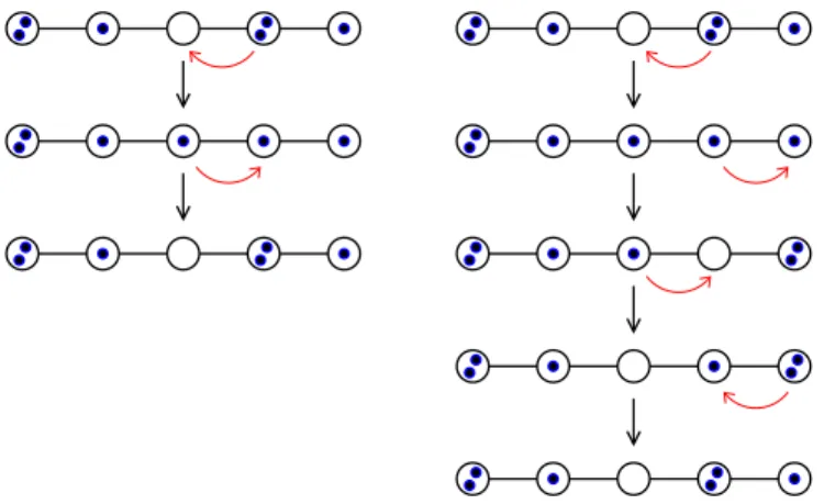
FIG. 1. (Color online) Sketch of a self-retracing (left column) and a non-self-retracing (right column) backscattered trajec- tiy in population space, for a Bose-Hubbard chain of five sites (marked by open black circles) containing altogether six particles (marked by filled blue circles). The curved (red) arrows indicate the imminent hopping event along the chain, while the vertical (black) arrows indicate the time evolution.

The self-retracing trajectory shown in the left column involves two hopping events, with one particle hopping to an adjacent site and back. A non-self-retracing backscattered trajectory within the chain, on the other hand, requires at least four hopping events. In the example shown on the right column, two atoms undergo hoppings to adjacent sites and back in an alternating order.

In the presence of time-reversal invariance, the backscattering probability P(n⁽ⁱ⁾,n⁽ⁱ⁾, t) contains additional contributions from pairs of backscattered trajectories γ, γ^′ where γ^′ = Tγ is the time reversal of γ.

Obviously, this requires that γ 6= Tγ, i.e., that γ is a non-self-retracing trajectory. In the limit of long evolution times t, self-retracing trajectories γ =Tγ generally represent a negligible minority among the set of all backscattered trajectories. Then we can safely assume that all backscattered trajectories arenon-self-retracing, which yields the semiclassical prediction

P¯(n⁽ⁱ⁾,n⁽ⁱ⁾, t) = 2 ¯P^cl(n⁽ⁱ⁾,n⁽ⁱ⁾, t) = 2X

γ

|A^(γ)|² (25) for the average quantum backscattering probability. The right column of Fig. 1 shows an example of such a non- self-retracing backscattered trajectory within the on-site population space, for the specific case of a Bose-Hubbard chain containing five sites. It involves four inter-site hoppings of particles along the chain.

For very short evolution times, on the contrary, the average quantum backscattering probability within such

a Bose-Hubbard chain is obviously dominated by contributions fromself-retracing trajectories, namely those trajectories in which one particle hops to an adjacent site and back, as shown in the left column of Fig. 1. Hence, for very short timest we obtain

P¯(n⁽ⁱ⁾,n⁽ⁱ⁾, t) = ¯P^cl(n⁽ⁱ⁾,n⁽ⁱ⁾, t) =X

γ

|A^(γ)|², (26) i.e., the classical and quantum backscattering probabili- ties are expected to agree with each other.

The crossover between the short-time behaviour given by Eq. (26) and the long-time behaviour given by Eq. (25) can generally be expressed as

P¯(n⁽ⁱ⁾,n⁽ⁱ⁾, t) = [1 +η(t)] ¯P^cl(n⁽ⁱ⁾,n⁽ⁱ⁾, t) (27) whereη(t) represents the relative frequency of non-self- retracing trajectories among the set of all backscattered trajectories at the evolution time t. This relative frequency depends on system-specific parameters, such as the relative interaction and disorder strengthsU/J and W/J, respectively, in our disordered Bose-Hubbard system. It can be quantitatively determined by means of the computation of classical trajectories within the Bose- Hubbard system under consideration, if a quantitative prediction of ¯P(n⁽ⁱ⁾,n⁽ⁱ⁾, t) is required in this crossover regime.

To provide an estimate for the relevant time scale that characterizes this crossover in the case of our Bose- Hubbard chain or ring systems, it is useful to note that at least four inter-site hoppings are required in order to accomplish a backscattered classical trajectory that is not identical to its time-reversed counterpart. In- deed, backscattered trajectories involving only two inter- site hoppings are necessarily self-retracing in population space, as the first hopping event has to be undone by the second hopping event in order to recover the initial distribution of populations, and a trajectory with exactly three inter-site hoppings cannot recover the initial distribution of populations at the end (except for a the special case of a three-site Bose-Hubbard ring) as those hoppings arise between adjacent sites only. De- noting by τ = ~/J the inverse Rabi frequency charac- terizing inter-site hoppings within the (non-interacting and disorder-free) Bose-Hubbard system, we can therefore roughly estimate this crossover time scale as 4τ,i.e., Eqs. (26) and (25) are predicted to be valid fort ≪4τ andt≫4τ, respectively. This prediction is found to be in good agreement with our numerical findings, as shown in Fig. 2 of the Letter.